
Analysis of Vertical Wind Shear Effects on Offshore Wind Energy Prediction Accuracy Applying Rotor Equivalent Wind Speed and the Relationship with Atmospheric Stability

 , , ,
, , ,  and
and
Abstract
:1. Introduction
2. Materials and Methods
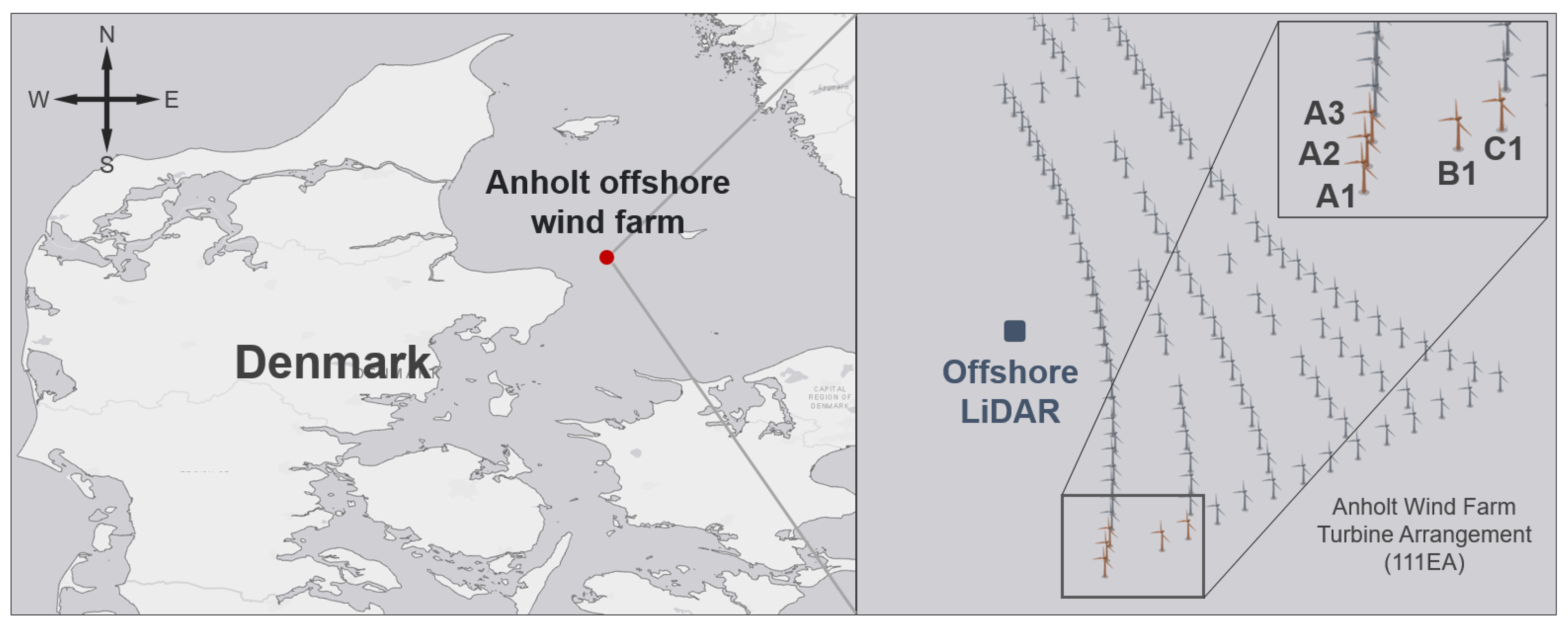
2.1. The Anholt Offshore Wind Farm
2.2. Offshore Wind LiDAR
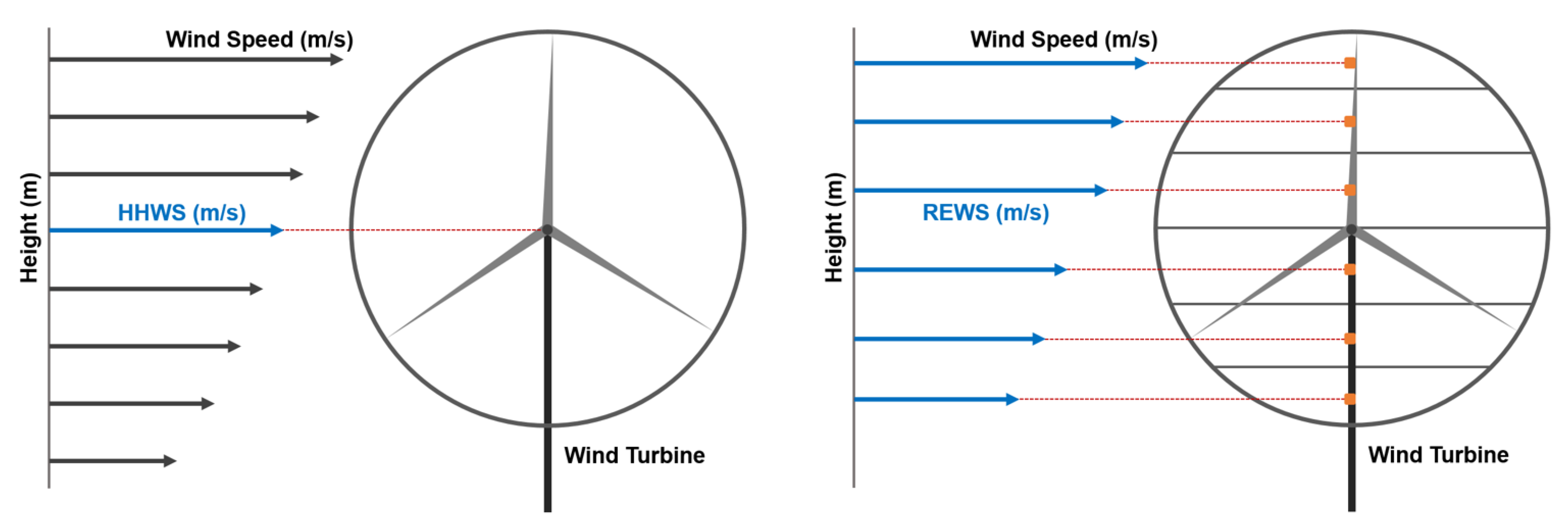
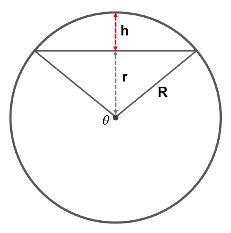
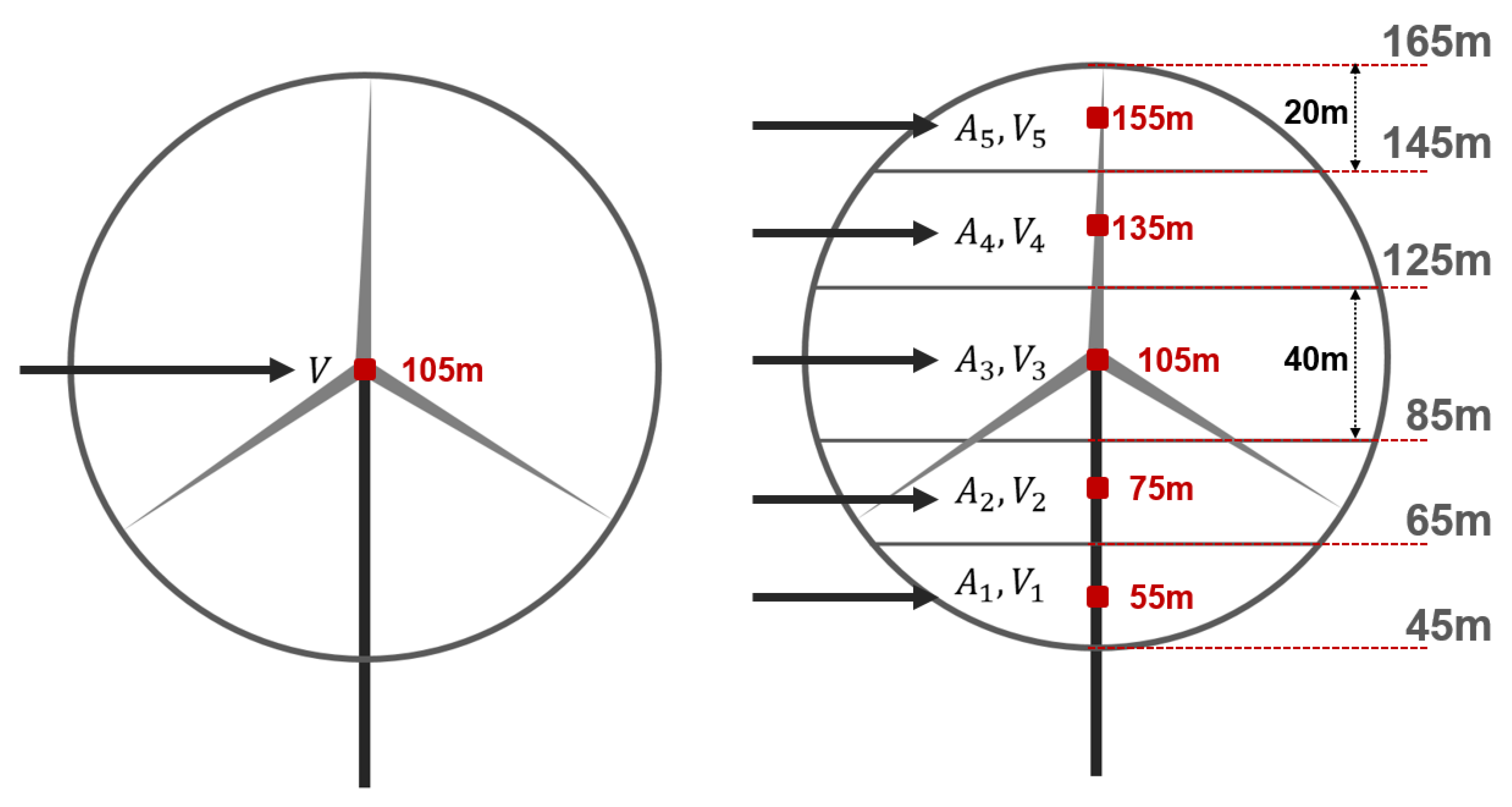
2.3. Rotor Equivalent Wind Speed
2.4. Atmospheric Stability
2.4.1. Wind Shear Exponent
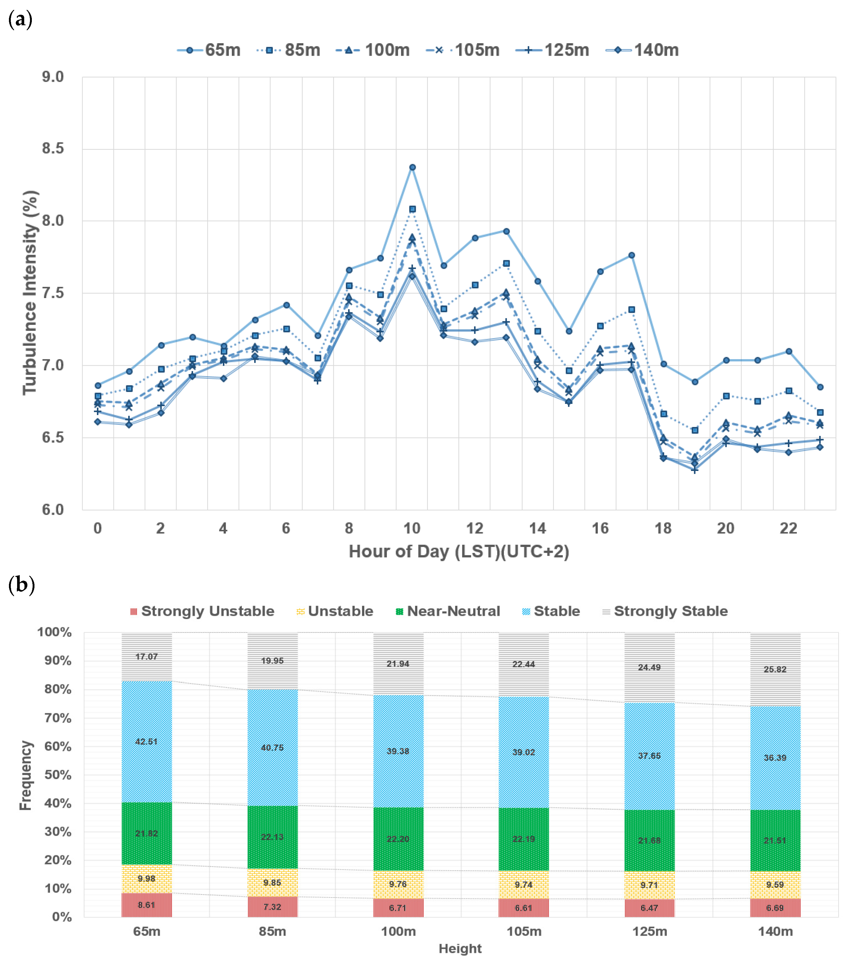
2.4.2. Turbulence Intensity (TI)
2.4.3. Richardson Number
2.5. WindSim
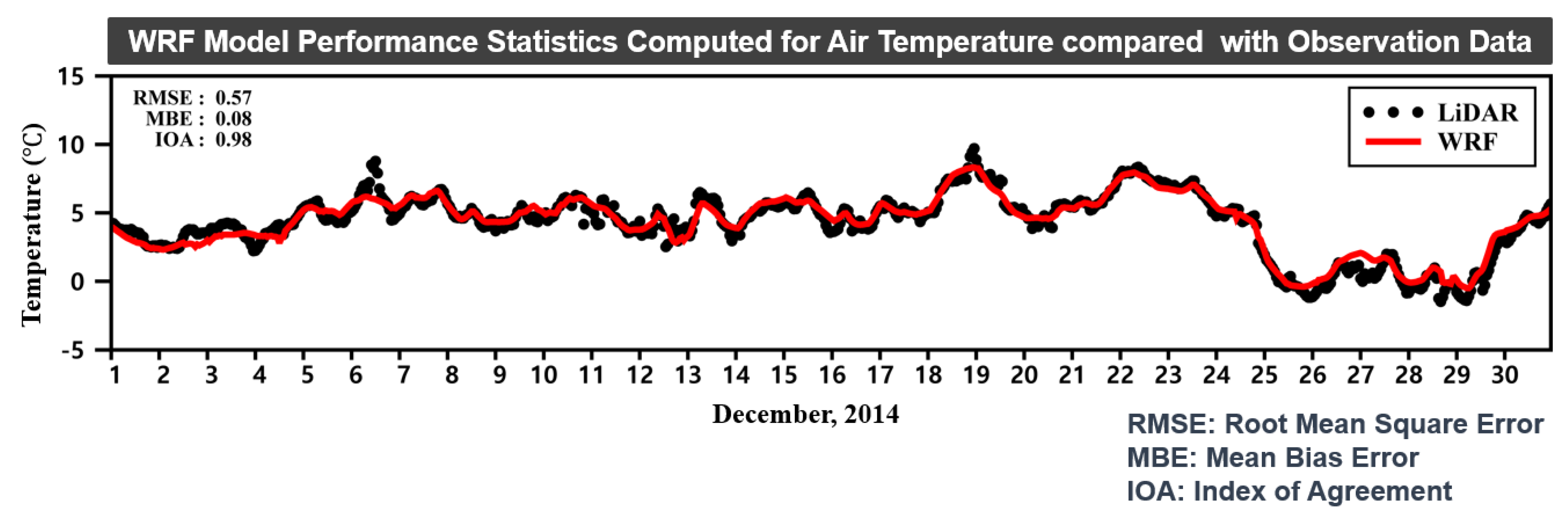
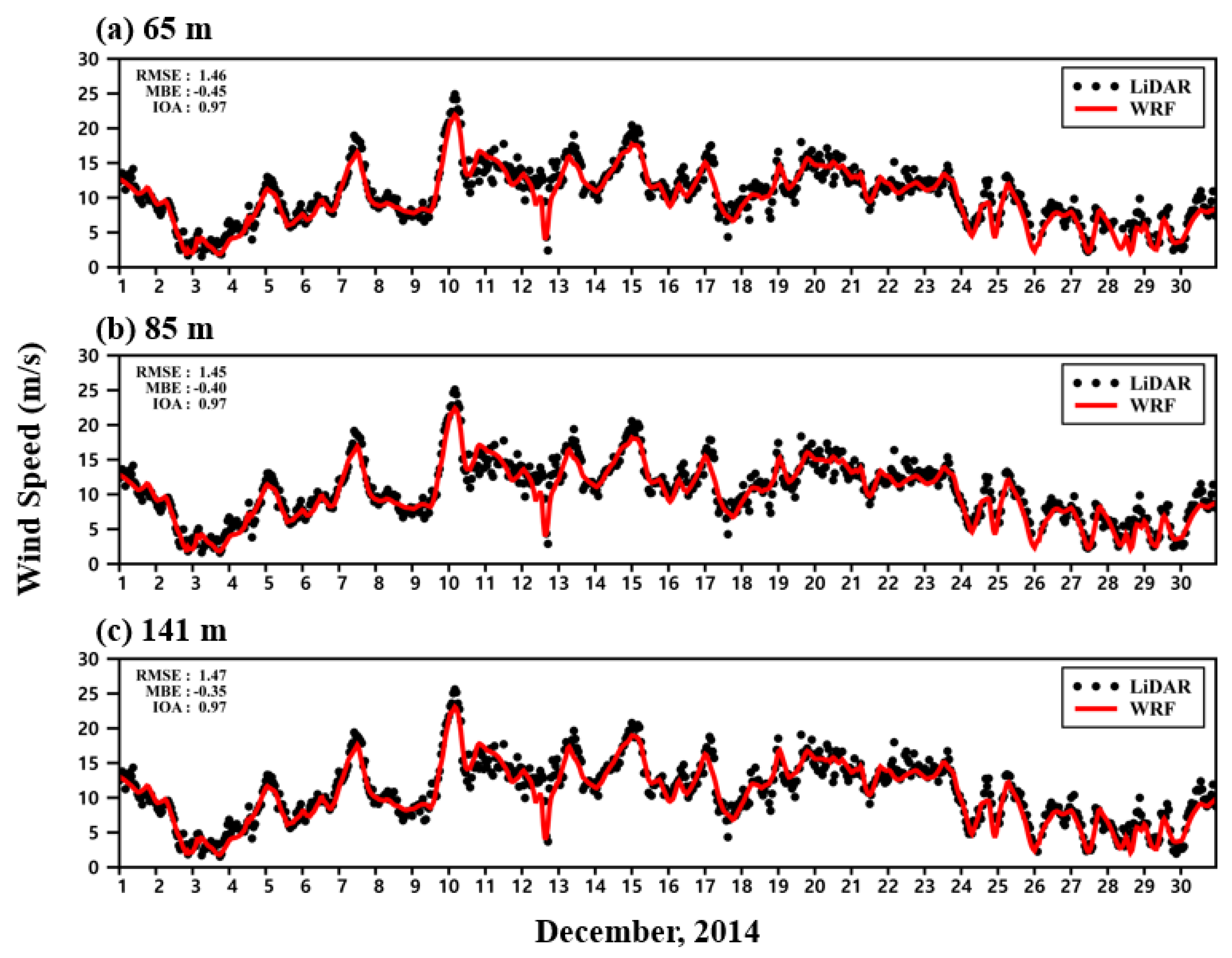
2.6. WRF
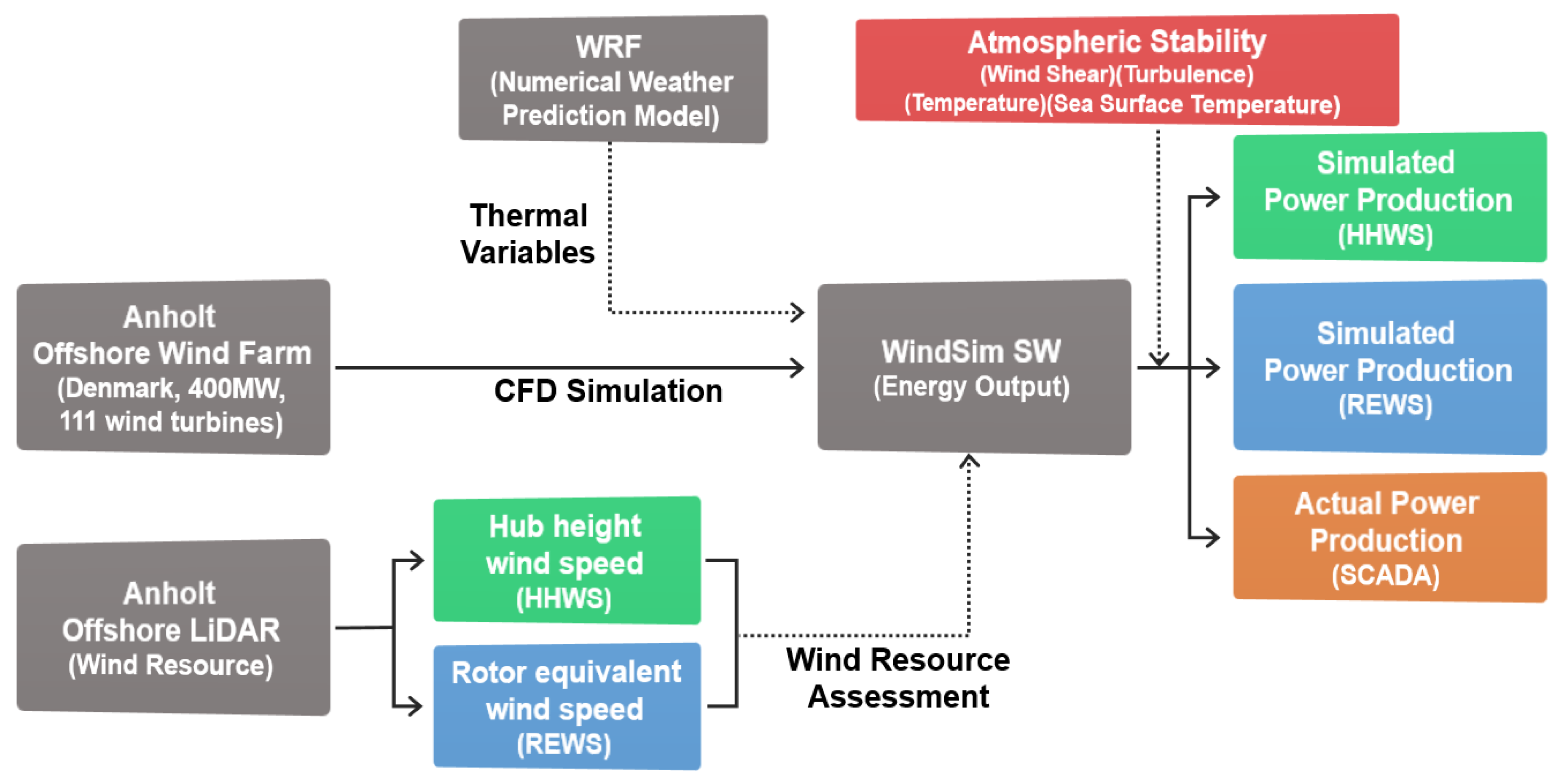
2.7. Study Procedure
3. Results
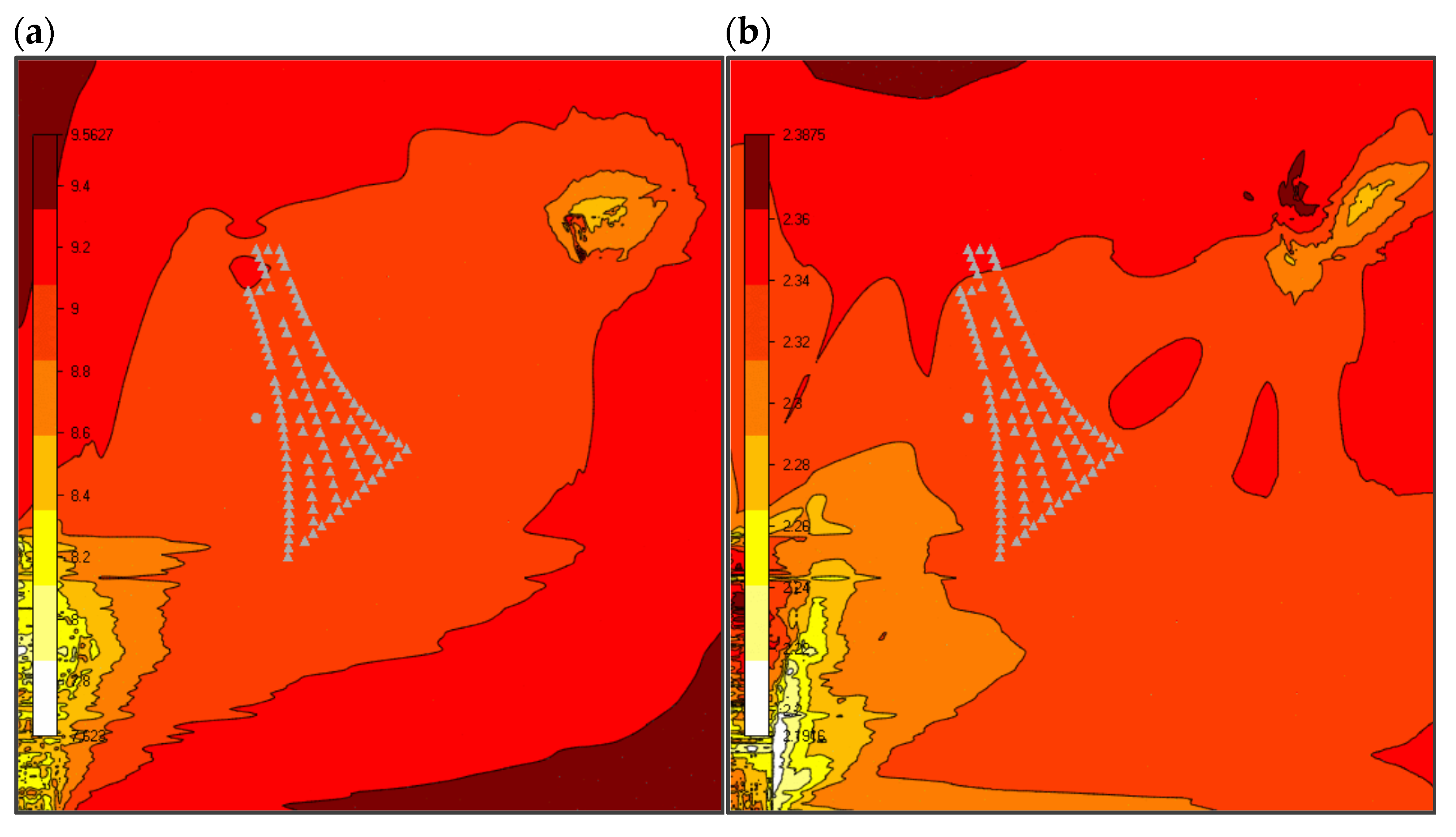
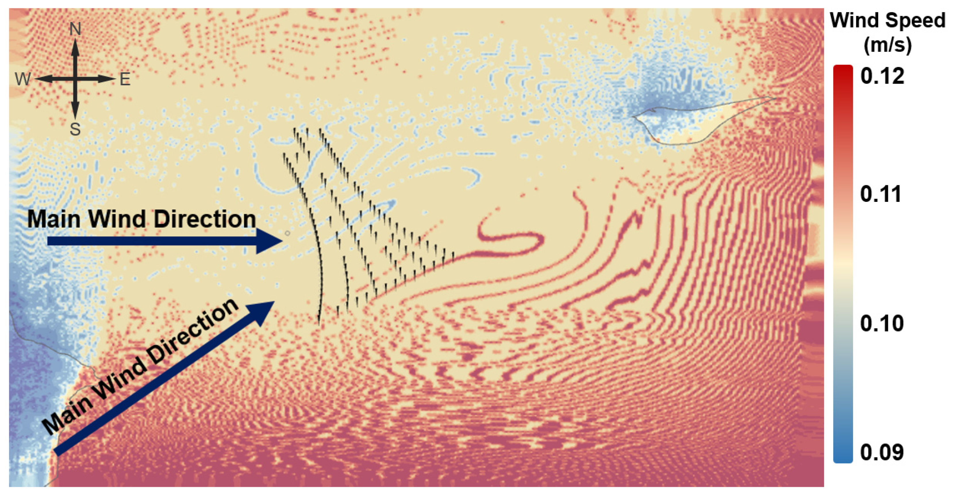
3.1. Model Simulation
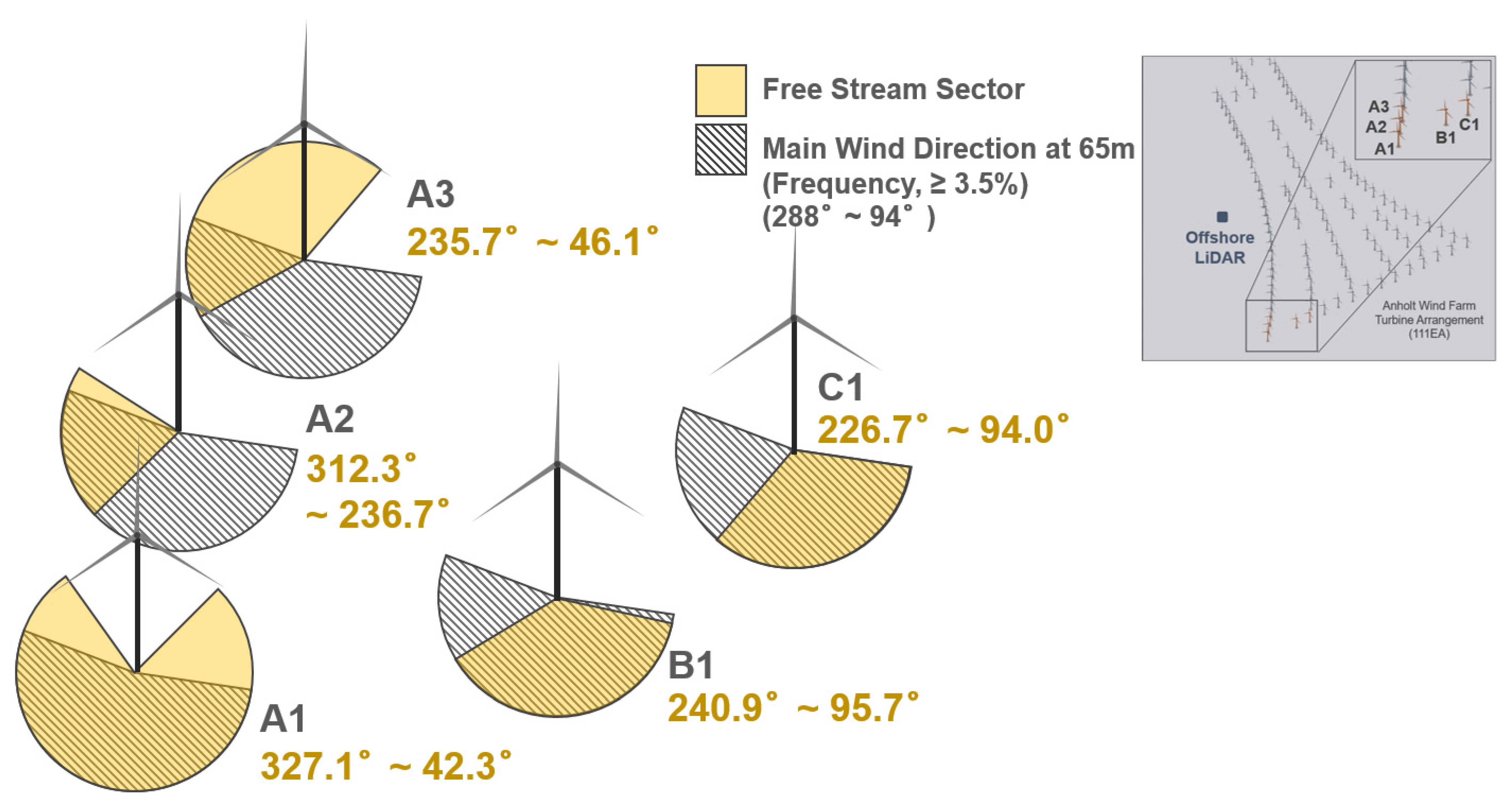
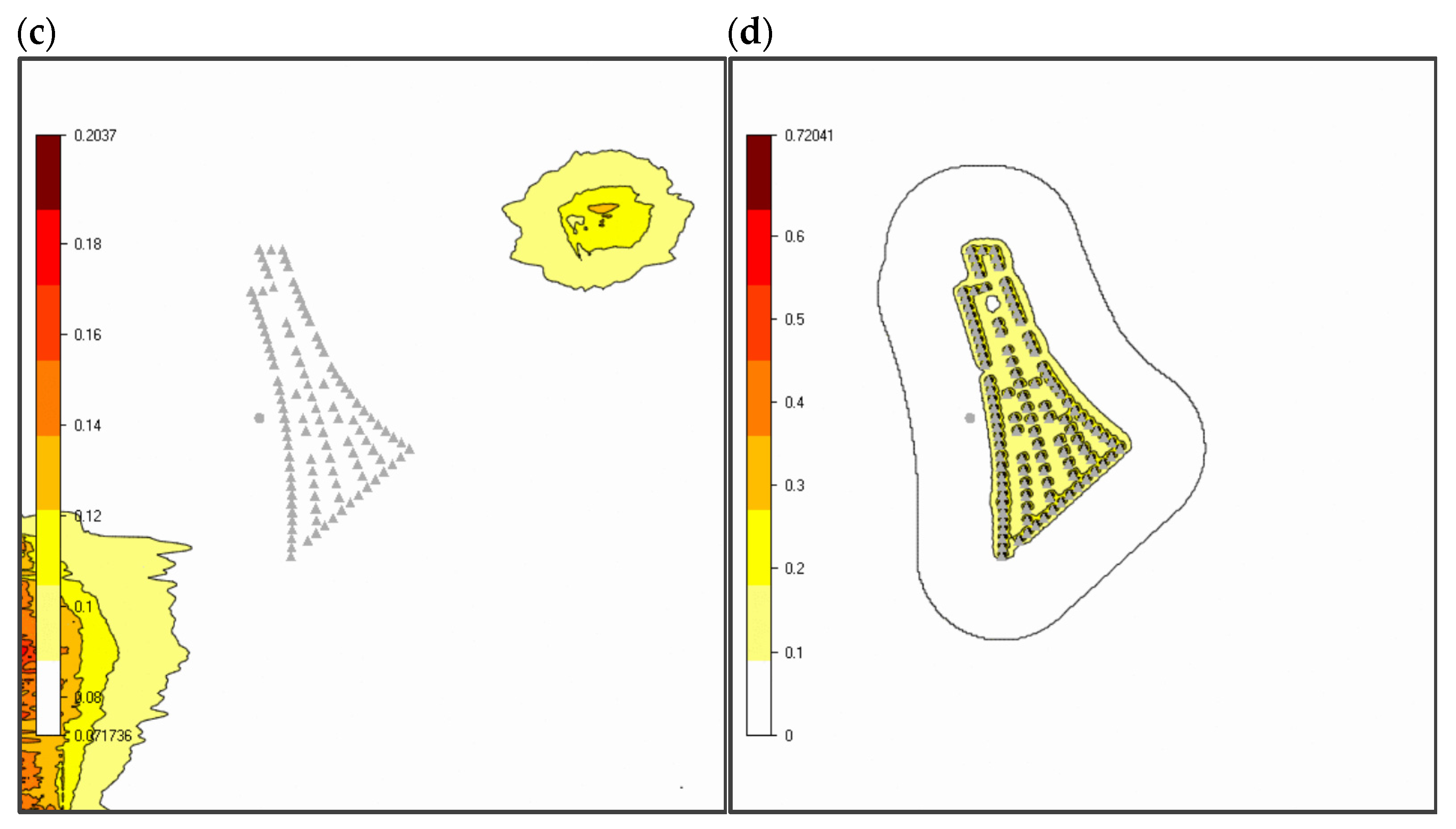
3.2. Stream Sector and Data Filtering
- Disturbed sector
- Rotor diameter at neighborhood wind turbine
- Distance between neighborhood wind turbine and target wind turbine
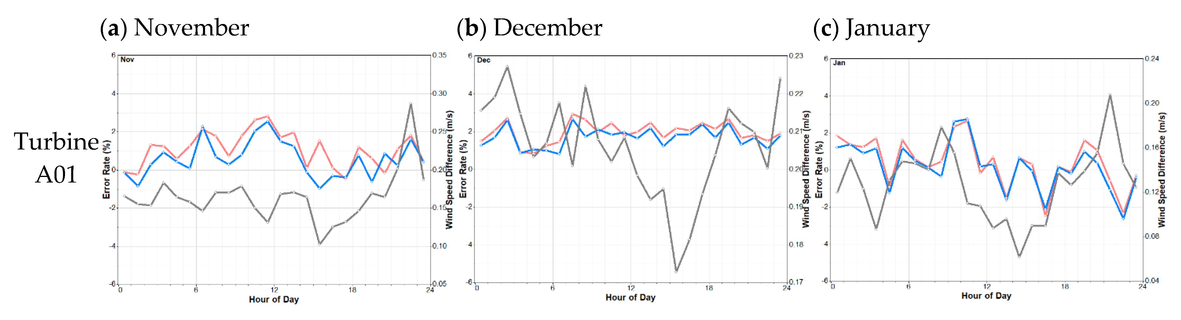
3.3. Comparison with Actual Data
3.3.1. Rotor Equivalent Wind Speed Calculation
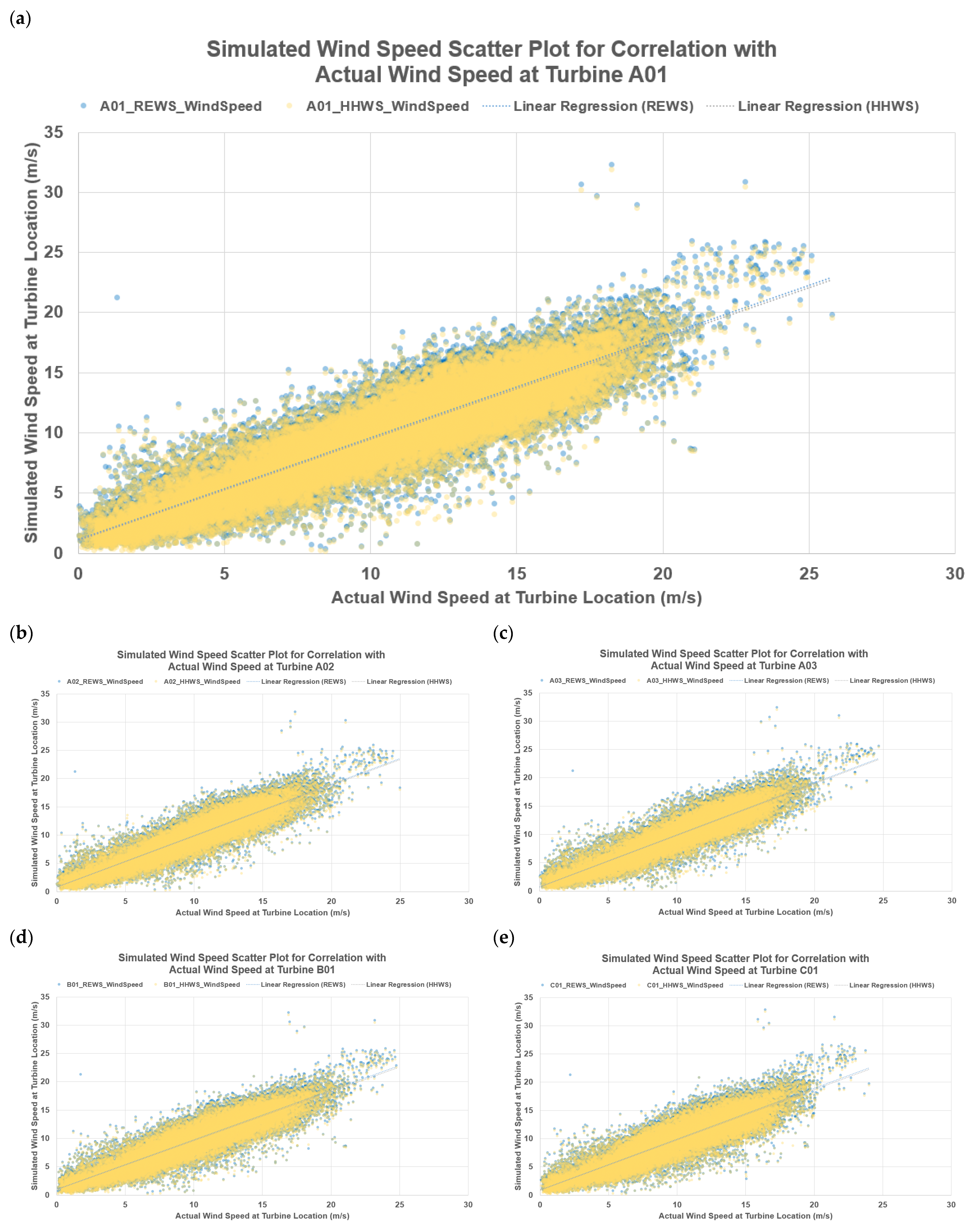
3.3.2. Comparison between HHWS and REWS
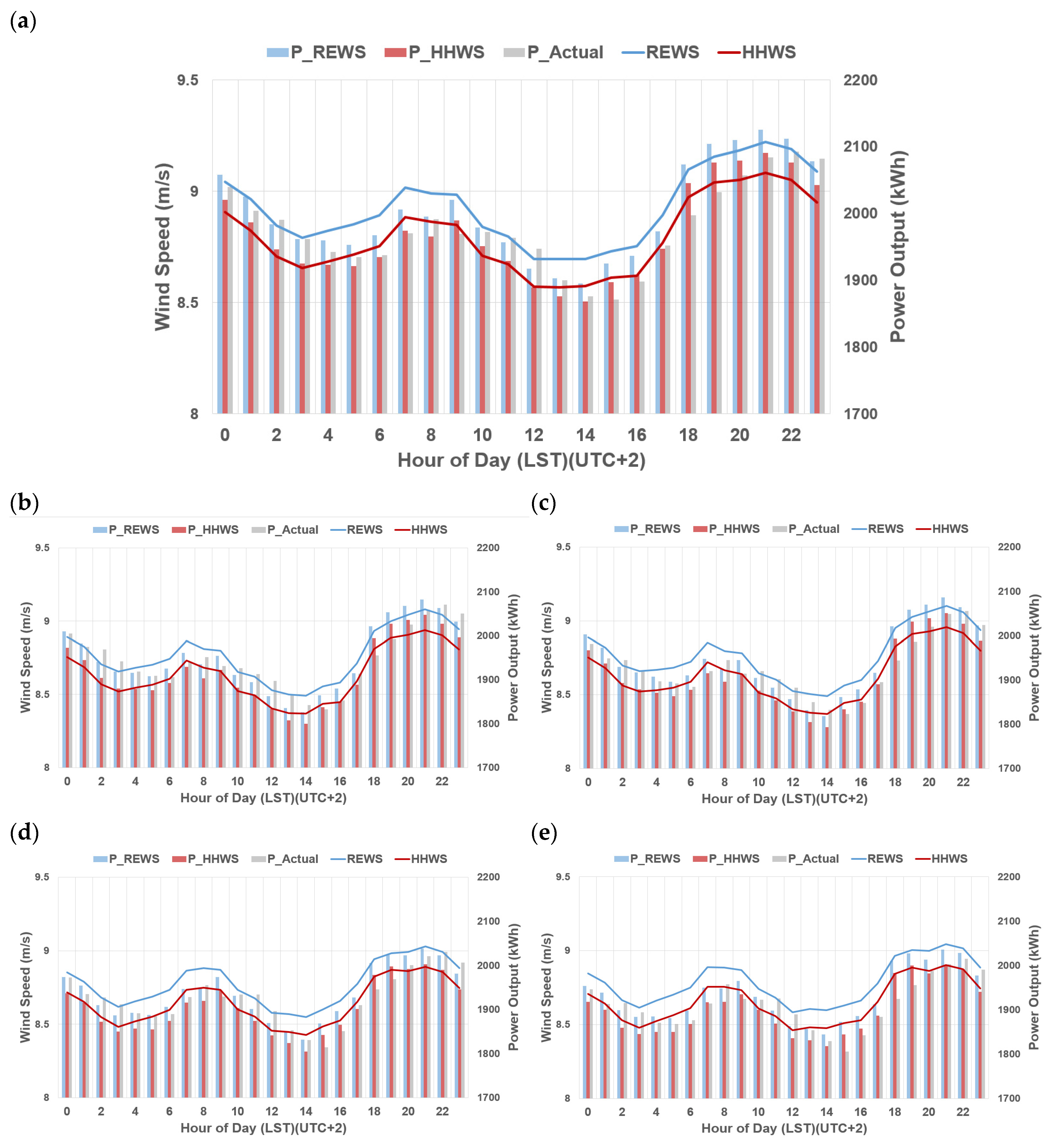
3.3.3. Comparison with Power Output
3.4. Atmospheric Stability in Anholt OWF
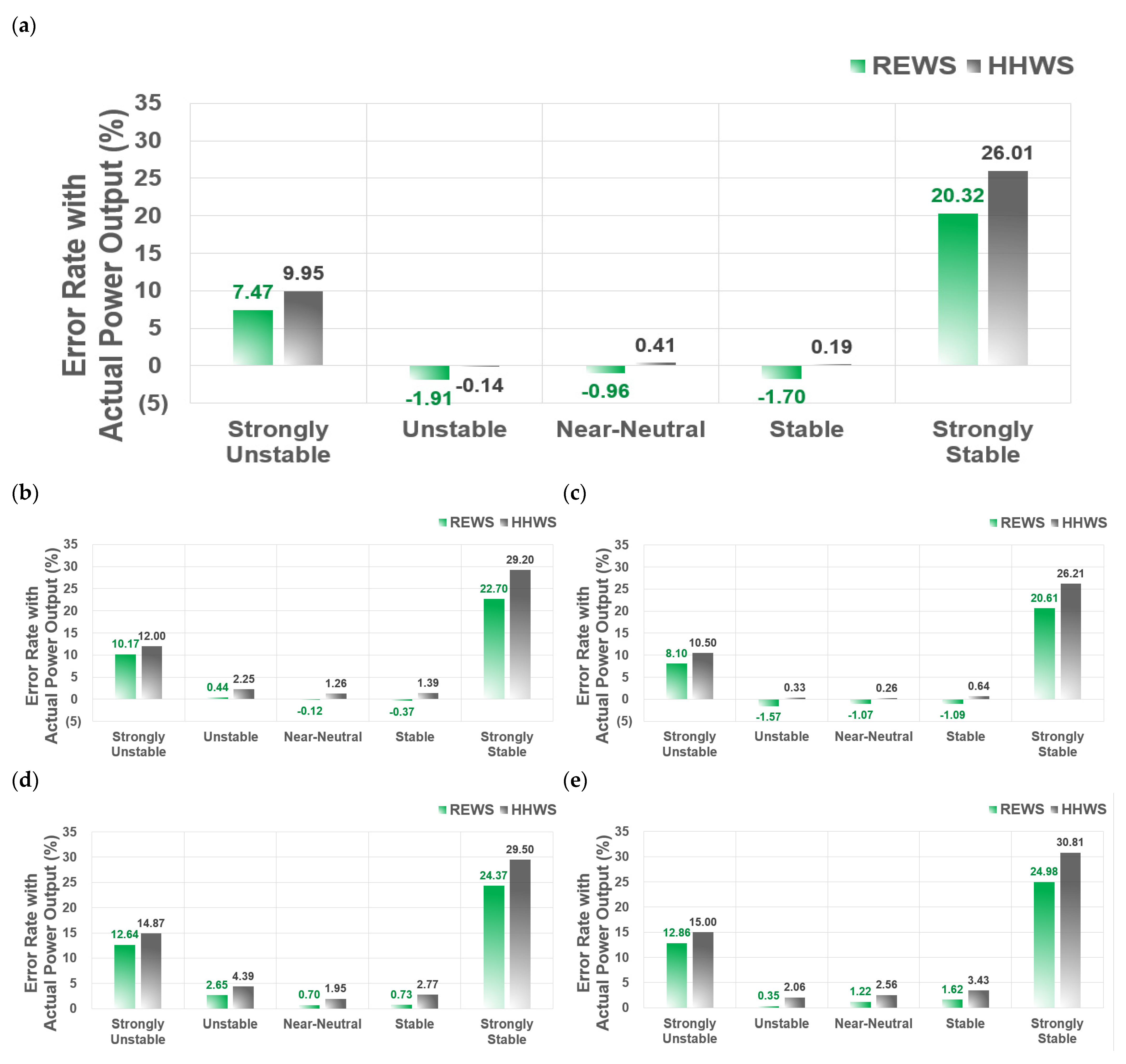
3.5. Power Output Related with Atmospheric Stability
4. Discussion
5. Conclusions
Author Contributions
Funding
Institutional Review Board Statement
Informed Consent Statement
Data Availability Statement
Acknowledgments
Conflicts of Interest
References
- Sovacool, B.K.; Griffiths, S.; Kim, J.; Bazilian, M. Climate Change and Industrial F-Gases: A Critical and Systematic Review of Developments, Sociotechnical Systems and Policy Options for Reducing Synthetic Greenhouse Gas Emissions. Renew. Sustain. Energy Rev. 2021, 141, 110759. [Google Scholar] [CrossRef]
- Nong, D.; Simshauser, P.; Nguyen, D.B. Greenhouse gas emissions vs CO2 emissions: Comparative analysis of a global carbon tax. Appl. Energy 2021, 298, 117223. Available online: https://www.sciencedirect.com/science/article/pii/S0306261921006462 (accessed on 15 April 2022). [CrossRef]
- O’Shaughnessy, E.; Heeter, J.; Shah, C.; Koebrich, S. Corporate Acceleration of the Renewable Energy Transition and Implications for Electric Grids. Renew. Sustain. Energy Rev. 2021, 146, 111160. [Google Scholar] [CrossRef]
- Murshed, M. Can Regional Trade Integration Facilitate Renewable Energy Transition to Ensure Energy Sustainability in South Asia? Energy Rep. 2021, 7, 808–821. [Google Scholar] [CrossRef]
- Meinshausen, M.; Lewis, J.; McGlade, C.; Gütschow, J.; Nicholls, Z.; Burdon, R.; Cozzi, L.; Hackmann, B. Realization of Paris Agreement Pledges May Limit Warming Just below 2 °C. Nature 2022, 604, 304–309. [Google Scholar] [CrossRef]
- Hwangbo, S.; Heo, S.; Yoo, C. Development of Deterministic-Stochastic Model to Integrate Variable Renewable Energy-Driven Electricity and Large-Scale Utility Networks: Towards Decarbonization Petrochemical Industry. Energy 2022, 238, 122006. [Google Scholar] [CrossRef]
- Chang, S.; Cho, J.; Heo, J.; Kang, J.; Kobashi, T. Energy Infrastructure Transitions with PV and EV Combined Systems Using Techno-Economic Analyses for Decarbonization in Cities. Appl. Energy 2022, 319, 119254. [Google Scholar] [CrossRef]
- Park, J.; Kim, B. An Analysis of South Korea’s Energy Transition Policy with Regards to Offshore Wind Power Development. Renew. Sustain. Energy Rev. 2019, 109, 71–84. [Google Scholar] [CrossRef]
- Alataş, S.; Karakaya, E.; Hiçyılmaz, B. What Does Input Substitution Tell Us in Helping Decarbonization and Dematerialization? Industry Level Analysis for South Korea. Sustain. Prod. Consum. 2021, 27, 411–424. [Google Scholar] [CrossRef]
- Jeong, W.-C.; Lee, D.-H.; Roh, J.H.; Park, J.-B. Scenario Analysis of the GHG Emissions in the Electricity Sector through 2030 in South Korea Considering Updated NDC. Energies 2022, 15, 3310. [Google Scholar] [CrossRef]
- Tran, T.-T.; Kim, E.; Lee, D. Development of a 3-Legged Jacket Substructure for Installation in the Southwest Offshore Wind Farm in South Korea. Ocean Eng. 2022, 246, 110643. [Google Scholar] [CrossRef]
- Ryu, G.H.; Kim, Y.-G.; Kwak, S.J.; Choi, M.S.; Jeong, M.-S.; Moon, C.-J. Atmospheric Stability Effects on Offshore and Coastal Wind Resource Characteristics in South Korea for Developing Offshore Wind Farms. Energies 2022, 15, 1305. [Google Scholar] [CrossRef]
- Chu, K.H.; Lim, J.; Mang, J.S.; Hwang, M.-H. Evaluation of Strategic Directions for Supply and Demand of Green Hydrogen in South Korea. Int. J. Hydrogen Energy 2022, 47, 1409–1424. [Google Scholar] [CrossRef]
- Chen, J.; Kim, M.-H. Review of Recent Offshore Wind Turbine Research and Optimization Methodologies in Their Design. J. Mar. Sci. Eng. 2022, 10, 28. [Google Scholar] [CrossRef]
- Wang, L.; Kolios, A.; Liu, X.; Venetsanos, D.; Rui, C. Reliability of Offshore Wind Turbine Support Structures: A State-of-the-Art Review. Renew. Sustain. Energy Rev. 2022, 161, 112250. [Google Scholar] [CrossRef]
- Pryor, S.C.; Barthelmie, R.J.; Shepherd, T.J. Wind Power Production from Very Large Offshore Wind Farms. Joule 2021, 5, 2663–2686. [Google Scholar] [CrossRef]
- Ren, Z.; Verma, A.S.; Li, Y.; Teuwen, J.J.E.; Jiang, Z. Offshore wind turbine operations and maintenance: A state-of-the-art review. Renew. Sustain. Energy Rev. 2021, 144, 110886. [Google Scholar] [CrossRef]
- Offshore Wind Turbines: Size Really Matters, Rystad Says. Offshore Engineer Magazine. 2020. Available online: https://www.oedigital.com/news/481796-offshore-wind-turbines-size-really-matters-rystad-says (accessed on 3 May 2022).
- Zhu, J.; Cai, X.; Ma, D.; Zhang, J.; Ni, X. Improved Structural Design of Wind Turbine Blade Based on Topology and Size Optimization. Int. J. Low-Carbon Technol. 2022, 17, 69–79. [Google Scholar] [CrossRef]
- Bilgili, M.; Tumse, S.; Tontu, M.; Sahin, B. Effect of Growth in Turbine Size on Rotor Aerodynamic Performance of Modern Commercial Large-Scale Wind Turbines. Arab. J. Sci. Eng. 2021, 46, 7185–7195. [Google Scholar] [CrossRef]
- Ryu, G.-H.; Kim, D.-H.; Lee, H.-W.; Park, S.-Y.; Yoo, J.-W.; Kim, H.-G. Accounting for the Atmospheric Stability in Wind Resource Variations and Its Impacts on the Power Generation by Concentric Equivalent Wind Speed. J. Korean Sol. Energy Soc. 2016, 36, 49–61. [Google Scholar] [CrossRef]
- Ryu, G.-H.; Kim, D.-H.; Lee, H.-W.; Park, S.-Y.; Kim, H.-G. A Study of Energy Production Change according to Atmospheric Stability and Equivalent Wind Speed in the Offshore Wind Farm using CFD Program. J. Environ. Sci. Int. 2016, 25, 247–257. [Google Scholar] [CrossRef]
- Scheurich, F.; Enevoldsen, P.B.; Paulsen, H.N.; Dickow, K.K.; Fiedel, M.; Loeven, A.; Antoniou, I. Improving the Accuracy of Wind Turbine Power Curve Validation by the Rotor Equivalent Wind Speed Concept. J. Phys. Conf. Ser. 2016, 753, 072029. [Google Scholar] [CrossRef] [Green Version]
- Van Sark, W.; Van der Velde, H.C.; Coelingh, J.P.; Bierbooms, W. Do we really need rotor equivalent wind speed? Wind Energy 2019, 22, 745–763. [Google Scholar] [CrossRef] [Green Version]
- Jeon, S.; Kim, B.; Huh, J. Study on methods to determine rotor equivalent wind speed to increase prediction accuracy of wind turbine performance under wake condition. Energy Sustain. Dev. 2017, 40, 41–49. [Google Scholar] [CrossRef]
- Wagner, R.; Antoniou, I.; Pedersen, S.M.; Courtney, M.S.; Jørgensen, H.E. The influence of the wind speed profile on wind turbine performance measurements. Wind Energy 2009, 12, 348–362. [Google Scholar] [CrossRef]
- IEC 61400-12-1; Wind Turbines-Part 12-1: Power Performance Measurements of Electricity Producing Wind Turbines. International Electrotechnical Commission: Geneva, Switzerland, 2005.
- Wharton, S.; Lundquist, J. Atmospheric stability effects wind turbine power collection. Environ. Res. Lett. 2012, 7, 014005. [Google Scholar] [CrossRef]
- DuPont, B.L.; Cagan, J.; Moriarty, P. Optimization of Wind Farm Layout and Wind Turbine Geometry Using a Multi-Level Extended Pattern Search Algorithm That Accounts for Variation in Wind Shear Profile Shape. In Proceedings of the ASME 2012 International Design Engineering Technical Conferences and Computers and Information in Engineering Conference, Chicago, IL, USA, 12–15 August 2012; American Society of Mechanical Engineers Digital Collection: New York, NY, USA, 2013; pp. 243–252. [Google Scholar] [CrossRef] [Green Version]
- Redfern, S.; Olson, J.B.; Lundquist, J.K.; Clack, C.T.M. Incorporation of the Rotor-Equivalent Wind Speed into the Weather Research and Forecasting Model’s Wind Farm Parameterization. Mon. Weather Rev. 2019, 147, 1029–1046. [Google Scholar] [CrossRef]
- Sasser, C.; Yu, M.; Delgado, R. Improvement of Wind Power Prediction from Meteorological Characterization with Machine Learning Models. Renew. Energy 2022, 183, 491–501. [Google Scholar] [CrossRef]
- Choukulkar, A.; Pichugina, Y.; Clack, C.T.M.; Calhoun, R.; Banta, R.; Brewer, A.; Hardesty, M. A New Formulation for Rotor Equivalent Wind Speed for Wind Resource Assessment and Wind Power Forecasting. Wind Energy 2016, 19, 1439–1452. [Google Scholar] [CrossRef]
- Bardal, L.M.; Sætran, L.R.; Wangsness, E. Performance Test of a 3MW Wind Turbine—Effects of Shear and Turbulence. Energy Procedia 2015, 80, 83–91. [Google Scholar] [CrossRef] [Green Version]
- Murphy, P.; Lundquist, J.K.; Fleming, P. How wind speed shear and directional veer affect the power production of a megawatt-scale operational wind turbine. Wind Energy Sci. 2020, 5, 1169–1190. [Google Scholar] [CrossRef]
- Zhan, L.; Letizia, S.; Valerio Iungo, G. LiDAR Measurements for an Onshore Wind Farm: Wake Variability for Different Incoming Wind Speeds and Atmospheric Stability Regimes. Wind Energy 2020, 23, 501–527. [Google Scholar] [CrossRef]
- Radünz, W.C.; Sakagami, Y.; Haas, R.; Petry, A.P.; Passos, J.C.; Miqueletti, M.; Dias, E. Influence of Atmospheric Stability on Wind Farm Performance in Complex Terrain. Appl. Energy 2021, 282, 116149. [Google Scholar] [CrossRef]
- Wise, A.S.; Neher, J.M.T.; Arthur, R.S.; Mirocha, J.D.; Lundquist, J.K.; Chow, F.K. Meso- to Microscale Modeling of Atmospheric Stability Effects on Wind Turbine Wake Behavior in Complex Terrain. Wind Energy Sci. 2022, 7, 367–386. [Google Scholar] [CrossRef]
- Han, X.; Liu, D.; Xu, C.; Shen, W.Z. Atmospheric Stability and Topography Effects on Wind Turbine Performance and Wake Properties in Complex Terrain. Renew. Energy 2018, 126, 640–651. [Google Scholar] [CrossRef]
- Kim, D.-Y.; Kim, Y.-H.; Kim, B.-S. Changes in Wind Turbine Power Characteristics and Annual Energy Production Due to Atmospheric Stability, Turbulence Intensity, and Wind Shear. Energy 2021, 214, 119051. [Google Scholar] [CrossRef]
- Guo, N.; Zhang, M.; Li, B.; Cheng, Y. Influence of Atmospheric Stability on Wind Farm Layout Optimization Based on an Improved Gaussian Wake Model. J. Wind Eng. Ind. Aerodyn. 2021, 211, 104548. [Google Scholar] [CrossRef]
- St. Martin, C.M.; Lundquist, J.K.; Clifton, A.; Poulos, G.S.; Schreck, S.J. Wind Turbine Power Production and Annual Energy Production Depend on Atmospheric Stability and Turbulence. Wind Energy Sci. 2016, 1, 221–236. [Google Scholar] [CrossRef] [Green Version]
- Peña, A.; Schaldemose Hansen, K.; Ott, S.; van der Laan, M.P. On Wake Modeling, Wind-Farm Gradients, and AEP Predictions at the Anholt Wind Farm. Wind Energy Sci. 2018, 3, 191–202. [Google Scholar] [CrossRef]
- Archer, C.L.; Vasel-Be-Hagh, A.; Yan, C.; Wu, S.; Pan, Y.; Brodie, J.F.; Maguire, A.E. Review and Evaluation of Wake Loss Models for Wind Energy Applications. Appl. Energy 2018, 226, 1187–1207. [Google Scholar] [CrossRef]


| Item | Content | |
|---|---|---|
| Offshore wind farm | Wind turbines | Siemens Gamesa Renewable Energy, SWT 3.6-120 |
| Number of wind turbines | 111 | |
| Wind turbine capacity [MW] | 3.6 | |
| Total capacity [MW] | 400 | |
| Hub height [m] | 81.6 | |
| Rotor diameter [m] | 120 | |
| Length of monopile [m] | 37–55 | |
| Water depth [m] | 15–19 | |
| Distance to shore [km] | 15 (Based on the nearest wind turbine) | |
| Offshore wind farm area [km2] | 88 | |
| Commissioned | Summer 2013 | |
| SCADA | Data | WTG 1 coordinates, SCADA data with min/max/mean/stddev 2 (Wind speed, Yaw position, Blade pitch position, RPM, Active power, Ambient temperature) |
| Item | Content | |
|---|---|---|
| Type | Leosphere WindCube | |
| Measurement period | 2013.01.01–2014.12.31 | |
| Height above MSL 1 [m] | 25.6 | |
| Location | 56.595664° N, 11.152728° E | |
| Observation height [m] | Wind speed | 40, 60, 76, 80, 100, 116, 160, 200, 250, 290 |
| Wind direction | 40, 60, 76, 80, 100, 116, 160, 200, 250, 290 | |
| Air pressure | 2 | |
| Relative humidity | 2 | |
| Air temperature | 2 | |
| Stability Class | Wind Shear | TI 1 | Richardson Number | Boundary Layer Properties |
|---|---|---|---|---|
| Strongly Unstable | < 0.0 | TI ≥ 0.15 | Ri < −0.86 | Lowest Wind Speed/Shear, Highly TI |
| Unstable | 0.0 ≤ < 0.1 | 0.11 ≤ TI < 0.15 | −0.86 ≤ Ri < −0.1 | Lower Wind Speed/Shear, High TI |
| Near-Neutral | 0.1 ≤ < 0.2 | 0.08 ≤ TI < 0.11 | −0.1 ≤ Ri < 0.053 | Logarithmic wind profile |
| Stable | 0.2 ≤ < 0.3 | 0.05 ≤ TI < 0.08 | 0.053 ≤ Ri < 0.134 | High Wind Speed/Shear, Nocturnal LLJ 2, Low TI |
| Strongly Stable | ≥ 0.3 | TI < 0.05 | Ri ≥ 0.134 | Highest Wind Speed/Shear, Nocturnal LLJ, Lowest TI |
| Category | Value |
|---|---|
| X range [UTM coord.] | 614,860.11–665,466.72 |
| Y range [UTM coord.] | 6,246,218.84–6,300,311.27 |
| Refinement | None |
| Height distribution factor | 0.1 |
| Grid spacing [m] | 120 |
| Number of cells | 3,120,500 |
| Number of cells in the Z direction | 20 |
| Speed above boundary layer [m/s] | 500 |
| Height of boundary layer [m] | 10 |
| Turbulence model | Standard k-epsilon |
| Number of iterations | 500 |
| SCADA Data Filtering Category | Wind Turbine | |||||||||
|---|---|---|---|---|---|---|---|---|---|---|
| A01 | A02 | A03 | B01 | C01 | ||||||
| Valid Data (#, %) | Data | % | Data | % | Data | % | Data | % | Data | % |
| Pre-Filtered Data | 104,584 | 100.0 | 104,584 | 100.0 | 104,584 | 100.0 | 104,584 | 100.0 | 104,584 | 100.0 |
| Wind Direction | 71,563 | 68.4 | 71,563 | 68.4 | 71,563 | 68.4 | 71,563 | 68.4 | 71,563 | 68.4 |
| (All) Wind Direction | 71,563 (68.4%) | |||||||||
| Missing Value | 102,958 | 98.4 | 104,318 | 99.7 | 104,559 | 99.9 | 104,216 | 99.9 | 104,480 | 99.9 |
| (All) Missing Value | 102,195 (97.7%) | |||||||||
| Cut in Speed, but Power ≤ 0 | 100,102 | 95.7 | 101,588 | 97.1 | 103,454 | 98.9 | 102,016 | 97.5 | 102,343 | 97.8 |
| (All) Cut in Speed but No Power | 91,113 (89.1%) | |||||||||
| Below Cut in Speed | 95,031 | 90.8 | 103,162 | 98.6 | 104,164 | 99.6 | 103,892 | 99.3 | 104,178 | 99.6 |
| (All) Below Cut in Speed | 92,091 (88.0%) | |||||||||
| Post-Filtered Data | 55,902 | 53.4 | 66,879 | 63.9 | 69,988 | 66.9 | 67,935 | 64.9 | 68,812 | 65.8 |
| All (Post Filtered Data) | 43,507 (41.6%) | |||||||||
| Sector | Wind Speed Height [m] | Wind Speed [m/s] | Segment Weighting [%] | Segment Bottom Height [m] | Segment Upper Height [m] | Segment Height [m] |
|---|---|---|---|---|---|---|
| A5 | 155 | 9.68 | 10.96 | 45 | 65 | 20 |
| A4 | 135 | 9.36 | 18.22 | 65 | 85 | 20 |
| A3 | 105 | 9.05 | 41.64 | 85 | 125 | 40 |
| A2 | 75 | 8.59 | 18.22 | 125 | 145 | 20 |
| A1 | 55 | 8.16 | 10.96 | 145 | 165 | 20 |
| Correlation (R2) | Turbine A01 | Turbine A02 | Turbine A03 | Turbine B01 | Turbine C01 |
|---|---|---|---|---|---|
| Actual Wind Speed vs. HHWS | 0.815 | 0.821 | 0.820 | 0.814 | 0.787 |
| Actual Wind Speed vs. REWS | 0.816 | 0.824 | 0.821 | 0.817 | 0.791 |
| Time (LST) | 0 | 1 | 2 | 3 | 4 | 5 | 6 | 7 | 8 | 9 | 10 | 11 | 12 | 13 | 14 | 15 | 16 | 17 | 18 | 19 | 20 | 21 | 22 | 23 | |
|---|---|---|---|---|---|---|---|---|---|---|---|---|---|---|---|---|---|---|---|---|---|---|---|---|---|
| >Actual Power | REWS | ● | ● | ● | ● | ● | ● | ● | ● | ● | ● | ● | ● | ● | ● | ● | ● | ||||||||
| HHWS | ● | ● | ● | ● | ● | ● | |||||||||||||||||||
| Abs. Diff. | REWS | ||||||||||||||||||||||||
| HHWS | |||||||||||||||||||||||||
| Stability Index | Turbine No. | Compared with REWS (Error Rate, %) | Compared with HHWS (Error Rate, %) | ||||||||
|---|---|---|---|---|---|---|---|---|---|---|---|
| 1 | 2 | 3 | 4 | 5 | 1 | 2 | 3 | 4 | 5 | ||
| Wind Shear | Turbine A01 | 7.47 | −1.91 | −0.96 | −1.70 | 20.32 | 9.95 | −0.14 | 0.41 | 0.19 | 26.01 |
| Turbine A02 | 10.17 | 0.44 | −0.12 | −0.37 | 22.70 | 12.00 | 2.25 | 1.26 | 1.39 | 29.20 | |
| Turbine A03 | 8.10 | −1.57 | −1.07 | −1.09 | 20.61 | 10.50 | 0.33 | 0.26 | 0.64 | 26.21 | |
| Turbine B01 | 12.64 | 2.65 | 0.70 | 0.73 | 24.37 | 14.87 | 4.39 | 1.95 | 2.77 | 29.50 | |
| Turbine C01 | 12.86 | 0.35 | 1.22 | 1.62 | 24.98 | 15.00 | 2.06 | 2.56 | 3.43 | 30.81 | |
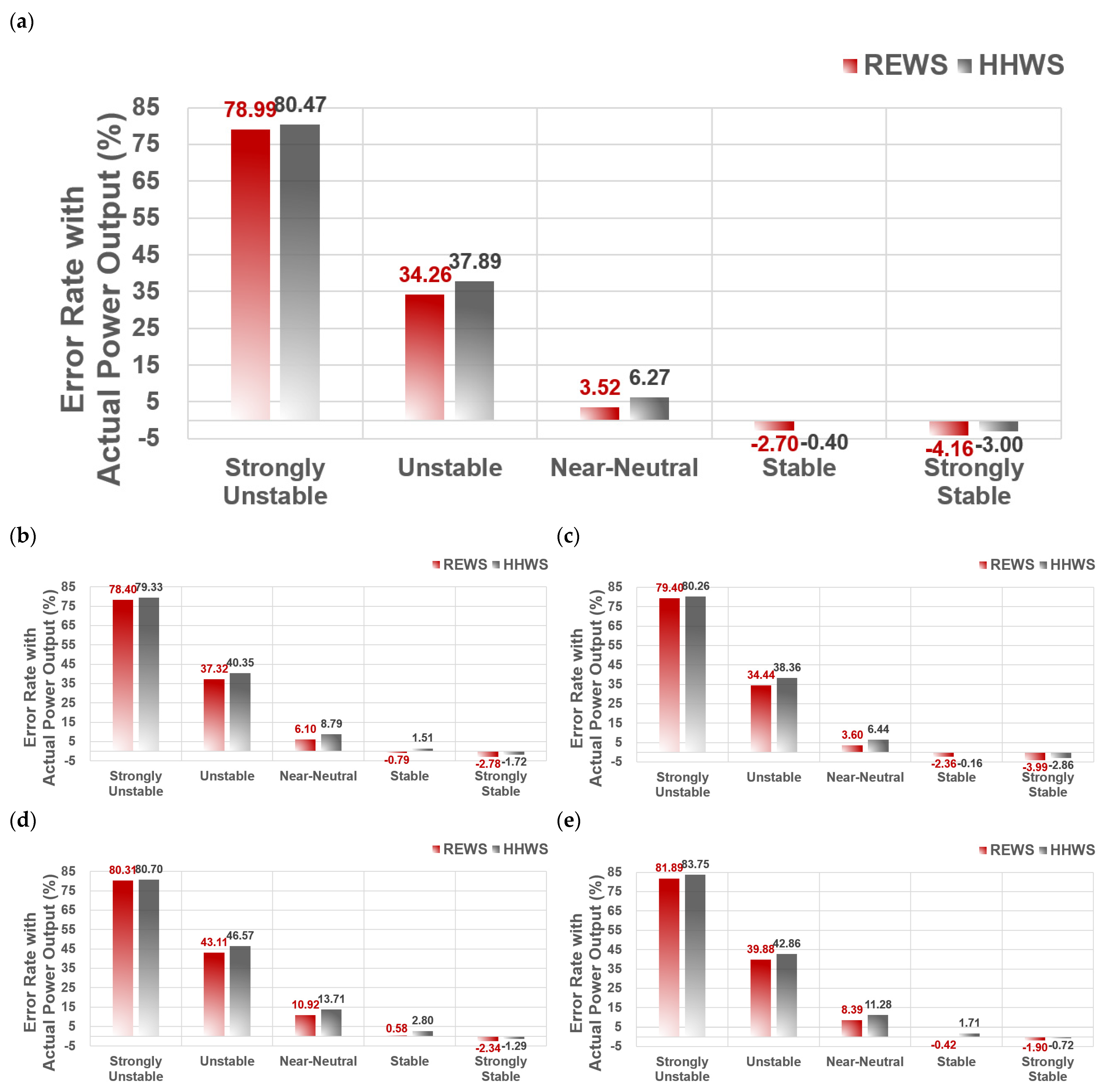
| TI | Turbine A01 | 78.99 | 34.26 | 3.52 | −2.70 | −4.16 | 80.47 | 37.89 | 6.27 | −0.40 | −3.00 |
| Turbine A02 | 78.40 | 37.32 | 6.10 | −0.79 | −2.78 | 79.33 | 40.35 | 8.79 | 1.51 | −1.72 | |
| Turbine A03 | 79.40 | 34.44 | 3.60 | −2.36 | −3.99 | 80.26 | 38.36 | 6.44 | −0.16 | −2.86 | |
| Turbine B01 | 80.31 | 43.11 | 10.92 | 0.58 | −2.34 | 80.70 | 46.57 | 13.71 | 2.80 | −1.29 | |
| Turbine C01 | 81.89 | 39.88 | 8.39 | −0.42 | −1.90 | 83.75 | 42.86 | 11.28 | 1.71 | −0.72 | |
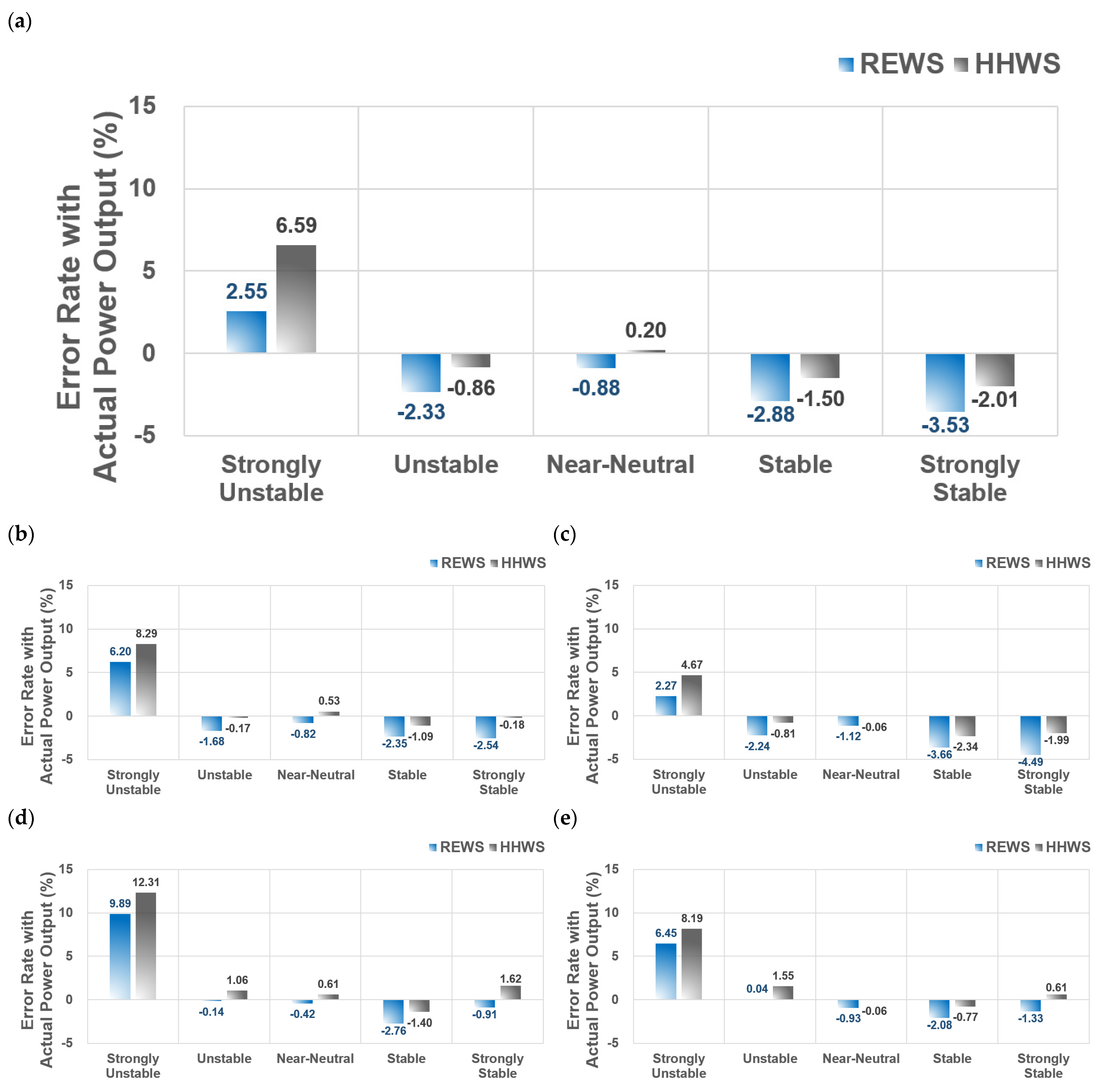
| Richardson Number | Turbine A01 | 2.55 | −2.33 | −0.88 | −2.88 | −3.53 | 6.59 | −0.86 | 0.20 | −1.50 | −2.01 |
| Turbine A02 | 6.20 | −1.68 | −0.82 | −2.35 | −2.54 | 8.29 | −0.17 | 0.53 | −1.09 | −0.18 | |
| Turbine A03 | 2.27 | −2.24 | −1.12 | −3.66 | −4.49 | 4.67 | −0.81 | −0.06 | −2.34 | −1.99 | |
| Turbine B01 | 9.89 | −0.14 | −0.42 | −2.76 | −0.91 | 12.31 | 1.06 | 0.61 | −1.40 | 1.62 | |
| Turbine C01 | 6.45 | 0.04 | −0.93 | −2.08 | −1.33 | 8.19 | 1.55 | −0.06 | −0.77 | 0.61 | |
Publisher’s Note: MDPI stays neutral with regard to jurisdictional claims in published maps and institutional affiliations. |
© 2022 by the authors. Licensee MDPI, Basel, Switzerland. This article is an open access article distributed under the terms and conditions of the Creative Commons Attribution (CC BY) license (https://creativecommons.org/licenses/by/4.0/).
Share and Cite
Ryu, G.H.; Kim, D.; Kim, D.-Y.; Kim, Y.-G.; Kwak, S.J.; Choi, M.S.; Jeon, W.; Kim, B.-S.; Moon, C.-J. Analysis of Vertical Wind Shear Effects on Offshore Wind Energy Prediction Accuracy Applying Rotor Equivalent Wind Speed and the Relationship with Atmospheric Stability. Appl. Sci. 2022, 12, 6949. https://doi.org/10.3390/app12146949
Ryu GH, Kim D, Kim D-Y, Kim Y-G, Kwak SJ, Choi MS, Jeon W, Kim B-S, Moon C-J. Analysis of Vertical Wind Shear Effects on Offshore Wind Energy Prediction Accuracy Applying Rotor Equivalent Wind Speed and the Relationship with Atmospheric Stability. Applied Sciences. 2022; 12(14):6949. https://doi.org/10.3390/app12146949
Chicago/Turabian StyleRyu, Geon Hwa, Dongjin Kim, Dae-Young Kim, Young-Gon Kim, Sung Jo Kwak, Man Soo Choi, Wonbae Jeon, Bum-Suk Kim, and Chae-Joo Moon. 2022. "Analysis of Vertical Wind Shear Effects on Offshore Wind Energy Prediction Accuracy Applying Rotor Equivalent Wind Speed and the Relationship with Atmospheric Stability" Applied Sciences 12, no. 14: 6949. https://doi.org/10.3390/app12146949
APA StyleRyu, G. H., Kim, D., Kim, D.-Y., Kim, Y.-G., Kwak, S. J., Choi, M. S., Jeon, W., Kim, B.-S., & Moon, C.-J. (2022). Analysis of Vertical Wind Shear Effects on Offshore Wind Energy Prediction Accuracy Applying Rotor Equivalent Wind Speed and the Relationship with Atmospheric Stability. Applied Sciences, 12(14), 6949. https://doi.org/10.3390/app12146949