
Solving Aggregate Production Planning Problems: An Extended TOPSIS Approach


Abstract
:1. Introduction
2. Literature Review
2.1. Robust Optimization
2.2. Mixed Integer/Integer Linear Programming
2.3. Nonlinear Programming
2.4. Fuzzy Mathematical Programming
2.5. Algorithms for Solving Large-Scale Problems
3. Problem Formulation
4. Model Solution
4.1. Distance Concept
4.2. TOPSIS for Solving MOP Problems
5. Model Implementation
5.1. Data Description
5.2. Problem Solving
5.3. Performance Analysis
6. Conclusions
Author Contributions
Funding
Institutional Review Board Statement
Informed Consent Statement
Data Availability Statement
Conflicts of Interest
References
- Baykasoglu, A. MOAPPS 1.0: Aggregate production planning using the multiple-objective tabu search. Int. J. Prod. Res. 2001, 39, 3685–3702. [Google Scholar] [CrossRef]
- Nam, S.-J.; Logendran, R. Aggregate production planning—A survey of models and methodologies. Eur. J. Oper. Res. 1992, 61, 255–272. [Google Scholar] [CrossRef]
- Yan, H.-S.; Zhang, X.-D.; Jiang, M. Hierarchical production planning with demand constraints. Comput. Ind. Eng. 2004, 46, 533–551. [Google Scholar] [CrossRef]
- Al-e-Hashem, S.M.J.M.; Malekly, H.; Aryanezhad, M.B. A multi-objective robust optimization model for multi-product multi-site aggregate production planning in a supply chain under uncertainty. Int. J. Prod. Econ. 2011, 134, 28–42. [Google Scholar] [CrossRef]
- Jamalnia, A.; Soukhakian, M.A. A hybrid fuzzy goal programming approach with different goal priorities to aggregate production planning. Comput. Ind. Eng. 2009, 56, 1474–1486. [Google Scholar] [CrossRef]
- Leung, S.C.H.; Wu, Y.; Lai, K.K. Multi-site aggregate production planning with multiple objectives: A goal programming approach. Prod. Plan. Control 2003, 14, 425–436. [Google Scholar] [CrossRef]
- Abo-Sinna, M.A.; Amer, A.H. Extensions of TOPSIS for multi-objective large-scale nonlinear programming problems. Appl. Math. Comput. 2005, 162, 243–256. [Google Scholar] [CrossRef]
- Holt, C.C.; Modigliani, F.; Simon, H.A. A linear decision rule for production and employment scheduling. Manag. Sci. 1955, 2, 1–30. [Google Scholar] [CrossRef]
- Guzman, E.; Andres, B.; Poler, R. Models and algorithms for production planning, scheduling and sequencing problems: A holistic framework and a systematic review. J. Ind. Inf. Integr. 2021; in press. [Google Scholar] [CrossRef]
- Jang, J.; Chung, B.D. Aggregate production planning considering implementation error: A robust optimization approach using bi-level particle swarm optimization. Comput. Ind. Eng. 2020, 142, 106367. [Google Scholar] [CrossRef]
- Attia, E.-A.; Megahed, A.; AlArjani, A.; Elbetar, A.; Duquenne, P. Aggregate production planning considering organizational learning with case based analysis. Ain Shams Eng. J. 2022, 13, 101575. [Google Scholar] [CrossRef]
- Mehdizadeh, E.; Niaki, S.T.A.; Hemati, M. A bi-objective aggregate production planning problem with learning effect and machine deterioration: Modeling and solution. Comput. Oper. Res. 2018, 91, 21–36. [Google Scholar] [CrossRef]
- Bakar, M.R.A.; Bakheet, A.J.K.; Kamil, F.; Kalaf, B.A.; Abbas, I.T.; Soon, L.L. Enhanced simulated annealing for solving aggregate production planning. Math. Probl. Eng. 2016, 2016, 1679315. [Google Scholar]
- Wang, S.-C.; Yeh, M.-F. A modified particle swarm optimization for aggregate production planning. Expert Syst. Appl. 2014, 41, 3069–3077. [Google Scholar] [CrossRef]
- Aazami, A.; Saidi-Mehrabad, M. Benders decomposition algorithm for robust aggregate production planning considering pricing decisions in competitive environment: A case study. Sci. Iran. 2019, 26, 3007–3031. [Google Scholar] [CrossRef] [Green Version]
- Yang, T.; Ignizio, J.P.; Kim, H.J. Fuzzy programming with nonlinear membership functions: Piecewise linear approximation. Fuzzy Sets Syst. 1991, 41, 39–53. [Google Scholar] [CrossRef]
- Khemiri, R.; Elbedoui-Maktouf, K.; Grabot, B.; Zouari, B. Integrating fuzzy TOPSIS and goal programming for multiple objective integrated procurement-production planning. In Proceedings of the 2017 22nd IEEE International Conference on Emerging Technologies and Factory Automation (ETFA), Limassol, Cyprus, 12–15 September 2017; pp. 1–8. [Google Scholar]
- Serhan, A.N.; Babaee, T.E. A systematic review of aggregate production planning literature with an outlook for sustainability and circularity. Environ. Dev. Sustain. 2022, 1–42. [Google Scholar] [CrossRef]
- Alazemi, F.K.A.O.H.; Ariffin, M.K.A.B.M.; Mustapha, F.B. A New Fuzzy TOPSIS-Based Machine Learning Framework forMinimizing Completion Time in Supply Chains. Int. J. Fuzzy Syst. 2022, 24, 1669–1695. [Google Scholar] [CrossRef]
- Leung, S.C.H.; Tsang, S.O.S.; Ng, W.L.; Wu, Y. A robust optimization model for multi-site production planning problem in an uncertain environment. Eur. J. Oper. Res. 2007, 181, 224–238. [Google Scholar] [CrossRef]
- Kazemi-Zanjani, M.; Ait-Kadi, D.; Nourelfath, M. Robust production planning in a manufacturing environment with random yield: A case in sawmill production planning. Eur. J. Oper. Res. 2010, 201, 882–891. [Google Scholar] [CrossRef]
- Dhaenens-Flipo, C.; Finke, G. An integrated model for an industrial production—Distribution problem. IIE Trans. 2001, 33, 705715. [Google Scholar] [CrossRef]
- Park, Y.B. An integrated approach for production and distribution planning in supply chain management. Int. J. Prod. Res. 2005, 43, 1205–1224. [Google Scholar] [CrossRef]
- da Silva, C.G.; Figueira, J.; Lisboa, J.; Barman, S. An interactive decision support system for an aggregate production planning model based on multiple criteria mixed integer linear programming. Omega 2006, 34, 167–177. [Google Scholar] [CrossRef] [Green Version]
- Rizk, N.; Martel, A.; D’amours, S. Synchronized production—Distribution planning in a single-plant multi-destination network. J. Oper. Res. Soc. 2008, 59, 90–104. [Google Scholar] [CrossRef]
- Chen, C.L.; Lee, W.C. Multi-objective optimization of multi-echelon supply chain networks with uncertain product demands and prices. Comput. Chem. Eng. 2004, 28, 1131–1144. [Google Scholar] [CrossRef]
- Lababidi, H.M.S.; Ahmed, M.A.; Alatiqi, I.M.; Al-Enzi, A.F. Optimizing the supply chain of a petrochemical company under uncertain operating and economic conditions. Ind. Eng. Chem. Res. 2004, 43, 63–73. [Google Scholar] [CrossRef]
- Wang, R.; Fang, H. Aggregate production planning with multiple objectives in a fuzzy environment. Eur. J. Oper. Res. 2001, 133, 521–536. [Google Scholar] [CrossRef]
- Fung, R.Y.K.; Tang, J.; Wang, D. Multiproduct aggregate production planning with fuzzy demands and fuzzy capacities. IEEE Trans. Syst. Man Cybern. Part A 2003, 33, 302–313. [Google Scholar] [CrossRef]
- Chen, S.-P.; Huang, W.-L. A membership function approach for aggregate production planning problems in fuzzy environments. Int. J. Prod. Res. 2010, 48, 7003–7023. [Google Scholar] [CrossRef]
- Pradenas, L.; Peñailillo, F.; Ferland, J. Aggregate production planning problem: A new algorithm. Electron. Notes Discret. Math. 2004, 18, 193–199. [Google Scholar] [CrossRef]
- Alieva, R.A.; Fazlollahi, B.; Guirimov, B.G.; Alievc, R.R. Fuzzy genetic approach to aggregate production—Distribution planning in supply chain management. Inf. Sci. 2007, 177, 4241–4255. [Google Scholar] [CrossRef]
- Jain, A.; Palekar, U.S. Aggregate production planning for a continuous reconfigurable manufacturing process. Comput. Oper. Res. 2005, 32, 1213–1236. [Google Scholar] [CrossRef]
- Ramezanian, R.; Rahmani, D.; Barzinpour, F. An aggregate production planning model for two phase production systems: Solving with genetic algorithm and tabu search. Expert Syst. Appl. 2012, 39, 1256–1263. [Google Scholar] [CrossRef]
- Freimer, M.; Yu, P.L. Some new results on compromise solutions for groupdecision problems. Manag. Sci. 1976, 22, 688–693. [Google Scholar] [CrossRef]
- Zare, H.; Kamali Saraji, M.; Tavana, M.; Streimikiene, D.; Cavallaro, F. An Integrated Fuzzy Goal Programming—Theory of Constraints Model for Production Planning and Optimization. Sustainability 2021, 13, 12728. [Google Scholar] [CrossRef]
- Ho, J.K.; Loute, E. Computational experience with advanced implementation of decomposition algorithm for linear programming. Math. Program. 1983, 27, 283–290. [Google Scholar] [CrossRef]
- Hwang, C.L.; Yoon, K. Multiple Attribute Decision Making: Methods and Applications; Springer: Berlin/Heidelberg, Germany, 1981. [Google Scholar]
- Lai, Y.-J.; Liu, T.-Y.; Hwang, C.-L. TOPSIS for MODM. Eur. J. Oper. Res. 1994, 76, 486–500. [Google Scholar] [CrossRef]
- Yu, P.L.; Zeleny, M. The set of all nondominated solutions in linear cases and a multicriteria decision making simplex method. J. Math. Anal. Appl. 1975, 49, 430–468. [Google Scholar] [CrossRef] [Green Version]
- Zeleny, M. Multiple Criteria Decision Making; McGraw-Hill: New York, NY, USA, 1982. [Google Scholar]
- Bellman, R.E.; Zadeh, L.A. Decision-making in a fuzzy environment. Manag. Sci. 1970, 17, 141–164. [Google Scholar] [CrossRef]
- Zimmermann, H.J. Fuzzy programming and linear programming with several objective functions. Fuzzy Sets Syst. 1978, 1, 45–55. [Google Scholar] [CrossRef]

| Product (i) | Sales Revenue (sri) | Production Costs, Regular Time (pci) | Production Costs, Overtime (oci) | Subcontracting Costs (sci) | Inventory Costs (cci) | Backorder Costs (bci) |
|---|---|---|---|---|---|---|
| 1 | 100 | 50 | 70 | 90 | 50 | 45 |
| 2 | 200 | 60 | 80 | 110 | 55 | 50 |
| Product (i) | Labor Time for Product | Machine Time |
Subcontracting Output Fraction |
Repair Cost | Defect Rate |
|---|---|---|---|---|---|
| 1 | 2 | 0.3 | 0.5 | 30 | 5% |
| 2 | 3 | 0.4 | 0.6 | 45 | 3% |
| Period (t) | ||||||
|---|---|---|---|---|---|---|
| 1 | 2 | 3 | 4 | 5 | 6 | |
| 450 | 500 | 350 | 550 | 400 | 500 | |
| 0.5 | 0.4 | 0.5 | 0.4 | 0.6 | 0.6 | |
| Period (t) | ||||||
|---|---|---|---|---|---|---|
| 1 | 2 | 3 | 4 | 5 | 6 | |
| Product: 1 (Wireless LAN) | ||||||
| Maximum forecast demand 1 | 6000 | 7000 | 5500 | 5000 | 4500 | 6000 |
| Minimum known demand 1 | 2000 | 2500 | 1500 | 1300 | 1000 | 2000 |
| Product: 2 (Ethernet Switch) | ||||||
| Maximum forecast demand 2 | 5500 | 6000 | 6500 | 4000 | 5000 | 3500 |
| Minimum known demand 2 | 1500 | 2000 | 2300 | 2000 | 1000 | 800 |
| Z1 | Z2 | Z3 | ||
|---|---|---|---|---|
| Max | Z1 | 9,500,000 + | 6,488,440 | 22,790 |
| Min | Z2 | 1,697,000 | 1,642,785 + | 3318 |
| Min | Z3 | 5,000,000 | 3,858,000 | 0 + |
| Z1 | Z2 | Z3 | ||
|---|---|---|---|---|
| Min | Z1 | 1,677,200 − | 1,654,480 | 3318 |
| Max | Z2 | 9,500,000 | 8,494,955 − | 18,389 |
| Max | Z3 | 7,776,000 | 5,183,500 | 33,930 − |
| Min | 1.35858 | 1.49444 |
| Max | 3.78877 | 1.43973 |
| Period (t) | ||||||
|---|---|---|---|---|---|---|
| 1 | 2 | 3 | 4 | 5 | 6 | |
| Product: 1 (Wireless LAN) | ||||||
| Regular time production | 734 | 753 | 128 | 633 | 485 | 305 |
| Overtime production | 10 | 102 | 194 | 207 | 26 | 127 |
| Subcontracting level | 2143 | 1662 | 1870 | 492 | 491 | 2978 |
| Inventory level | 0 | 0 | 0 | 0 | 0 | 0 |
| Backorder level | 0 | 0 | 0 | 0 | 0 | 0 |
| Product: 2 (Ethernet Switch) | ||||||
| Regular time production | 61 | 207 | 848 | 0 | 743 | 871 |
| Overtime production | 317 | 240 | 3 | 88 | 97 | 156 |
| Subcontracting level | 5122 | 5553 | 5661 | 3900 | 2721 | 2290 |
| Inventory level | 0 | 0 | 12 | 0 | 0 | 0 |
| Backorder level | 0 | 0 | 0 | 0 | 1439 | 1622 |
| Workforce level | 450 | 500 | 350 | 550 | 400 | 500 |
| Hiring | 0 | 50 | 0 | 200 | 0 | 100 |
| Laying off | 50 | 0 | 150 | 0 | 150 | 0 |
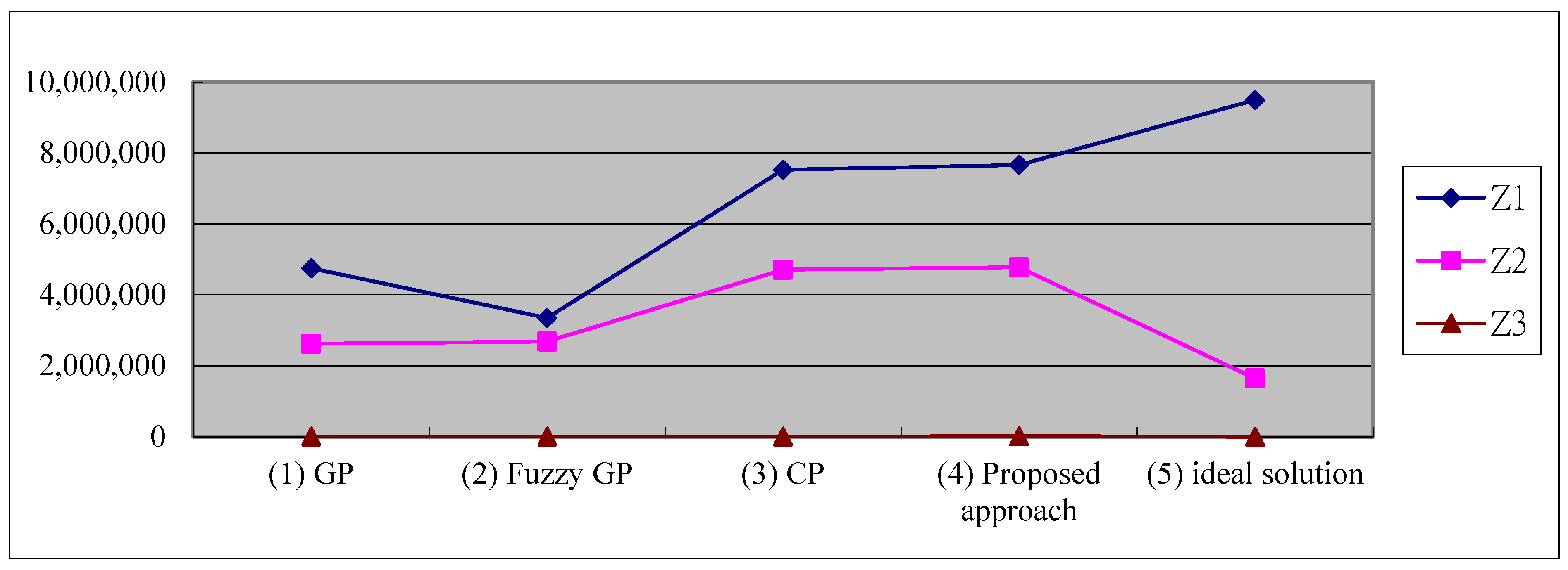
| (a) GP | (b) Fuzzy GP | (c) CP | (d) Proposed Approach | (e) Optimal Solution | |
|---|---|---|---|---|---|
| 4,750,000 | 3,350,000 | 7,530,000 | 7,662,900 | 9,500,000 | |
| 2,616,120 | 2,679,250 | 4,706,250 | 4,779,525 | 1,642,785 | |
| 3785 | 3785 | 1019 | 10,458 | 0 | |
| Profit | 2,130,095 | 666,965 | 2,822,731 | 2,872,917 | - |
| 0.8116 | 1.1504 | 0.5999 | 0.5928 | - | |
| 0.5123 | 0.8017 | 0.3729 | 0.3714 | - | |
| 0.4000 | 0.7343 | 0.3000 | 0.3000 | - |
Publisher’s Note: MDPI stays neutral with regard to jurisdictional claims in published maps and institutional affiliations. |
© 2022 by the authors. Licensee MDPI, Basel, Switzerland. This article is an open access article distributed under the terms and conditions of the Creative Commons Attribution (CC BY) license (https://creativecommons.org/licenses/by/4.0/).
Share and Cite
Yu, V.F.; Kao, H.-C.; Chiang, F.-Y.; Lin, S.-W. Solving Aggregate Production Planning Problems: An Extended TOPSIS Approach. Appl. Sci. 2022, 12, 6945. https://doi.org/10.3390/app12146945
Yu VF, Kao H-C, Chiang F-Y, Lin S-W. Solving Aggregate Production Planning Problems: An Extended TOPSIS Approach. Applied Sciences. 2022; 12(14):6945. https://doi.org/10.3390/app12146945
Chicago/Turabian StyleYu, Vincent F., Hsuan-Chih Kao, Fu-Yuan Chiang, and Shih-Wei Lin. 2022. "Solving Aggregate Production Planning Problems: An Extended TOPSIS Approach" Applied Sciences 12, no. 14: 6945. https://doi.org/10.3390/app12146945
APA StyleYu, V. F., Kao, H.-C., Chiang, F.-Y., & Lin, S.-W. (2022). Solving Aggregate Production Planning Problems: An Extended TOPSIS Approach. Applied Sciences, 12(14), 6945. https://doi.org/10.3390/app12146945