Computer Vision System: Measuring Displacement and Bending Angle of Ionic Polymer-Metal Composites

Featured Application

The proposed vision system can be used to measure the displacement and bending angle of ionic polymer–metal composites (IPMCs).

Abstract

A computer vision system for measuring the displacement and bending angle of ionic polymer–metal composites (IPMC) was proposed in this study. The logical progression of measuring IPMC displacement and bending angle was laid out. This study used Python (version 3.10) in conjunction with OpenCV (version 4.5.5.64) for the development of the vision system. The coding functions and the mathematical formulas used were elaborated on. IPMC contour detection was discussed in detail, along with appropriate camera and lighting setups. Measurements generated from the vision system were compared to approximated values via a manual calculation method. Good agreement was found between the results produced by the two methods. The mean absolute error (MAE) and root mean squared error (RMSE) for the displacement values are 0.068080668 and 0.088160652, respectively, and 0.081544205 and 0.103880163, respectively, for the bending angle values. The proposed vision system can accurately approximate the displacement and bending angle of IPMCs.

1. Introduction

Electroactive polymers (EAPs) are currently the closest in emulating natural muscles, earning the moniker artificial muscle for some [1,2,3]. EAPs deform in response to an electric field [1]. Known for their high power-to-weight ratio, EAPs are relatively new and require extensive research to establish a grounded understanding of their basic principles and what parameters control their electro-activation behaviour [3,4]. Ionic polymer–metal composites (IPMCs) are a subset of EAPs known for their sensing and actuating abilities [1]. The general structure of an IPMC consists of a polymer membrane sandwiched between metal electrodes. Nafion, a perfluorinated sulfonic-acid (PFSA) ionomer developed and trademarked by DuPont, is commonly used as the polymer membrane for IPMCs, with platinum as the electrodes [1]. One method of characterising IPMC behaviour is to measure its displacement under voltage loading. This study looks at proposing a computer vision system to measure this displacement along with its bending angle.

Measuring the displacement of IPMCs entails looking at the tip-to-tip displacement of the composite under various voltage loadings, usually from 1 V to 10 V. Two methods of measuring displacement are generally found in literature: measurement using a camera or using a laser displacement sensor [5,6,7,8,9,10,11,12,13,14,15,16]. Some studies combine both methods, interchanging them depending on how large the displacement and bending angle is [17].

The setup using a laser displacement sensor is relatively simple, with the sensor outputting displaced values as the voltage is varied. A disadvantage to laser displacement sensors is that they can only measure linear tip displacement, which could not accurately map the curved bending response exhibited by IPMCs [5]. Furthermore, laser sensors are also affected by changes in beam refraction, making them unsuitable for uses in underwater or humid conditions as well as on highly-reflective objects [11,12]. Also, depending on the resolution of the sensor used, accuracy may vary. Studies utilising this configuration only use it for small displacements where the curvature is negligible. For larger displacements, many opt for the other method of using a digital camera.

The general setup utilising a digital camera is as shown in Figure 1. The setup consists of a camera placed some distance from the clamped sample, against a marked background. As voltage is applied, the IPMC bends from the negatively charged side to the positively charged side. This bending is recorded by the camera, and the displacement can be determined from the still frames captured, using the marked background as reference.

Displacement values of the IPMC are calculated using basic trigonometry in this setup. Referring to the triangle with sides xyz in Figure 2, the tip-to-tip displacement can be calculated using Pythagoras’s theorem. Similarly, trigonometric laws such as the Cosine Law can be used to find the bending angle.

Manually calculating the displacement and bending angle for a few IPMC samples is practical when dealing with a small sample size, for example 3 s bending footage of one IPMC sample shot at 50 frames per second will have 150 frames. However, this becomes repetitive, cumbersome and problematic when the sample is large, possibly ranging from hundreds to thousands of samples. Manually calculating such sizes is unrealistic and will lead to errors and extended work hours. Thus, a more pragmatic approach would be to automate this process through a computer vision system. Computer vision is related to the analysis, modification and high-level understanding of digital images or videos [18]. This idea is not new, with the earliest mention of a setup by Cohen et al. [13,14] in which a system was developed to visualise and measure tip displacement of IPMCs using a charge-coupled device (CCD) camera. The use of an edge detection algorithm was mentioned, but details were not elaborated on.

Another similar system using a CCD camera was explored by Tsiakmakis et al. [11,12]. In this study the authors proposed an image processing system to measure IPMC displacement for underwater micro-robotic applications. The algorithm was written in C++, with the main focus of the setup being the detection of low frequency, large displacements of IPMCs. The image processing techniques used and the logic employed to detect the tip of the IPMCs were elaborated on. However, the code was not made available, and no mention was made of the code being open source.

2. Computer Vision System

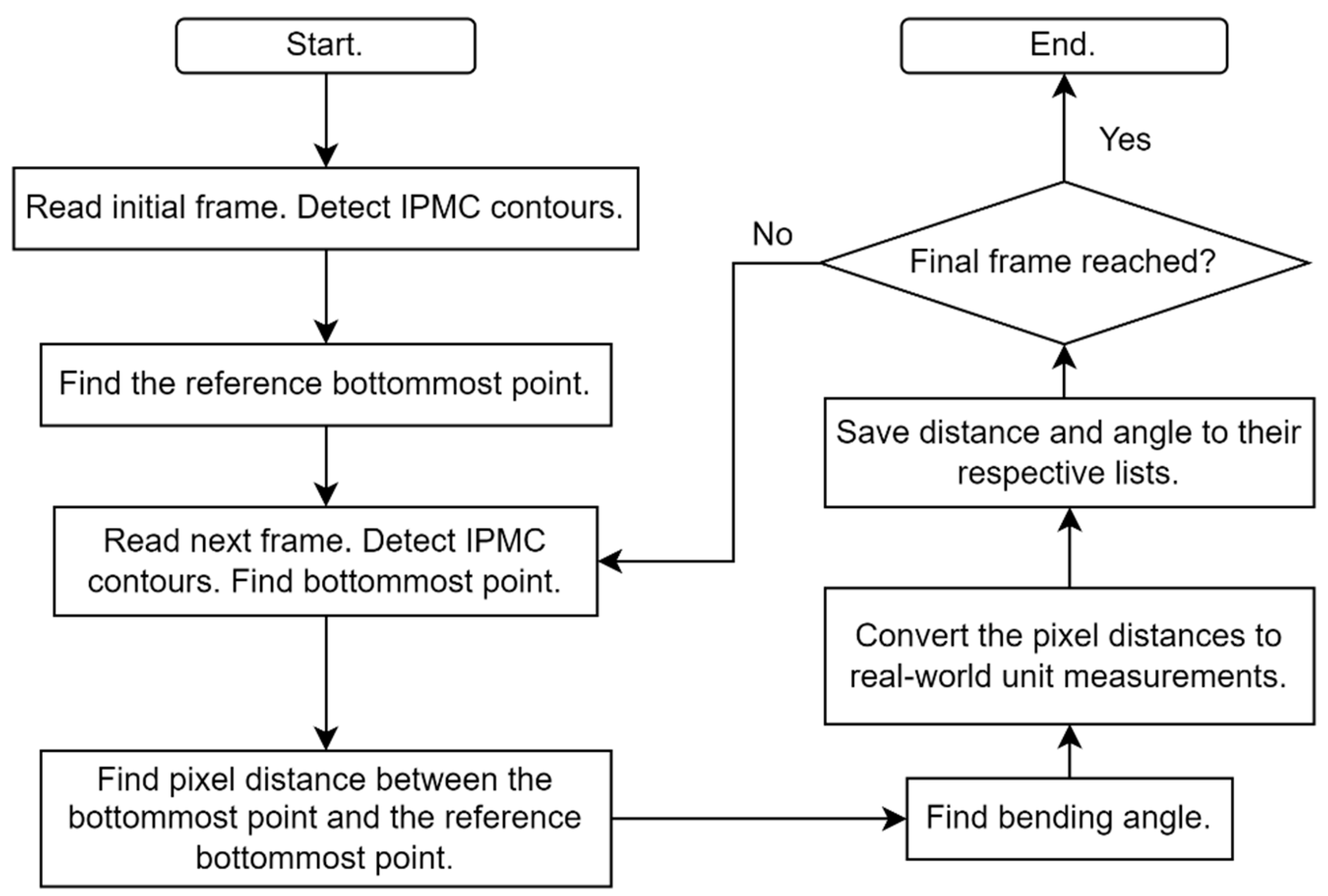
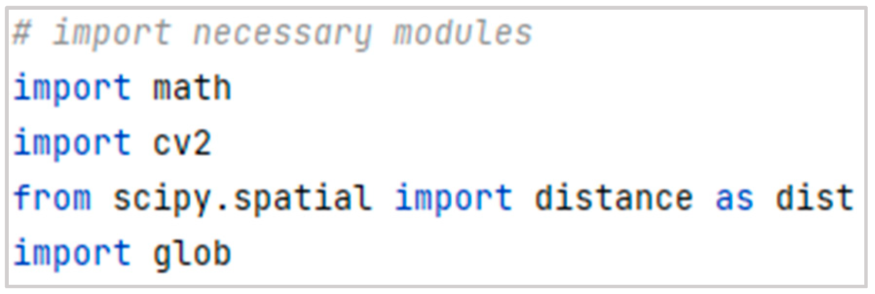
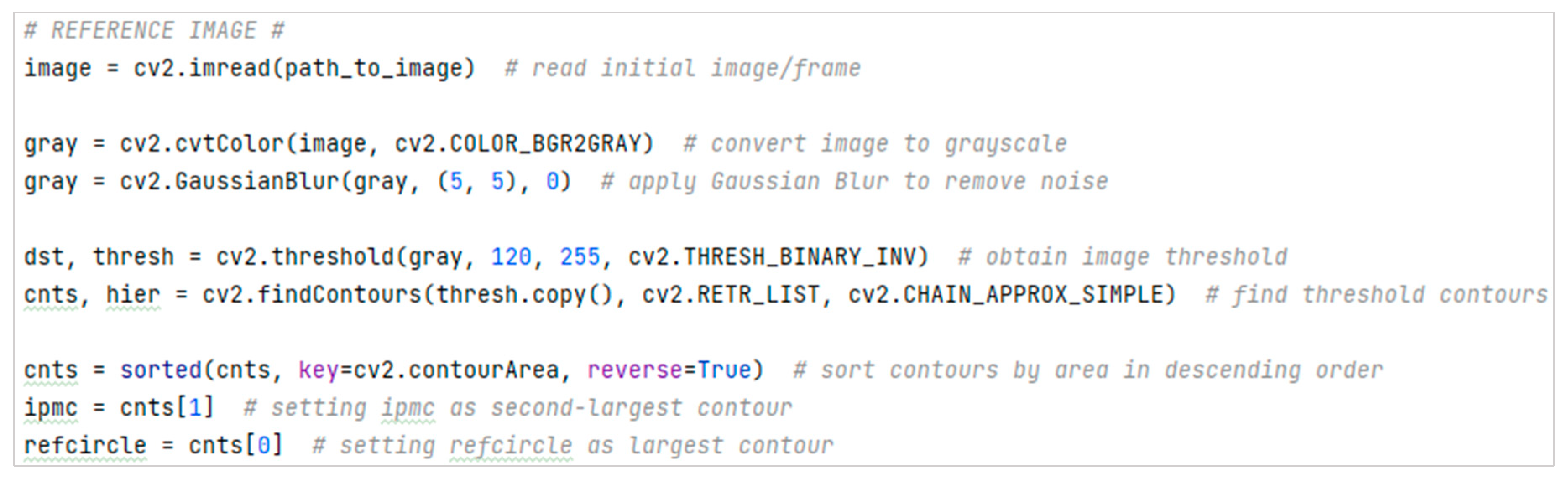
The computer vision system in this study aims to identify the IPMC sample and map out its displacement and bending angle and is comprised of two components: the programme or coding and the camera configuration.

OpenCV (version 4.5.5.64, Intel, Santa Clara, CA, USA), an open-source computer vision library, will be utilised for this system in conjunction with Python (version 3.10, Python Software Foundation, Wilmington, DE, USA). OpenCV contains a large number of functions; from low-level image processing functions, such as noise removal and contrast enhancement, to high-level functions, such as face detection and object tracking [18]. The logical progression of the vision system to measure the tip-to-tip displacement and bending angle of IPMCs is given in Figure 3.

2.1. Code Overview

The code for this research was written using Python (version 3.10, Python Software Foundation) utilising OpenCV (version 4.5.5.64, Intel). This section will give a high-level description of the functionality and function calls within the code. A fully commented file is available on GitHub (link provided in the Supplementary Materials section).

Initially, the necessary modules were imported as shown in Figure 4. Their functionalities are as follows; math module—access to mathematical functions to be used later as part of bending angle calculation; cv2 module—access to the image processing techniques in OpenCV; scipy.spatial.distance module—access to distance matrix computation to calculate the Euclidean distance between points; and glob module—used to locate directories.

Two Python lists were created: one to store the displacement values and the other for the bending angle values. The width of the reference circle was also defined. Next, the initial image was loaded and processed using the OpenCV module (cv2). Images were converted to grayscale and Gaussian blur was applied to reduce image noise. Finally, threshold and contours were identified and sorted (see Figure 5).

The topmost point and bottommost point of the IPMC in the initial frame were identified, and the Euclidean distance between these points was calculated (Figure 6).

The diameter of the reference circle was identified by locating the leftmost and the rightmost points of the circle. The Euclidean pixel distance between the two points was calculated and was divided by the width of the circle in millimetres (50 mm) to obtain the pixel-to-millimetre ratio. Subsequent images were then located and processed using a for-loop.

The bottommost point of the IPMC was located in the subsequent images (Figure 7). The Euclidean distances between this point and the reference topmost and bottommost points were calculated. IPMC displacement in millimetres, denoted by d2, was found by diving variable c with the pixel-to-millimetre ratio. The calculated value was then stored in the previously defined list for displacement values.

Bending angle was calculated using the Cosine Law (see Figure 8). The arccosine of the bending angle (γ) was computed using the math.acos() function from the Math module. After converting the angle to degrees, the value was stored in the bending angle list.

The code will loop until all the specified images have been analysed. Values stored in the displacement and bending angle lists were written to text files. The following sections will go into more detail about the functionalities mentioned in this section. Open access to the fully commented code is available on GitHub (link provided in the Supplementary Materials section).

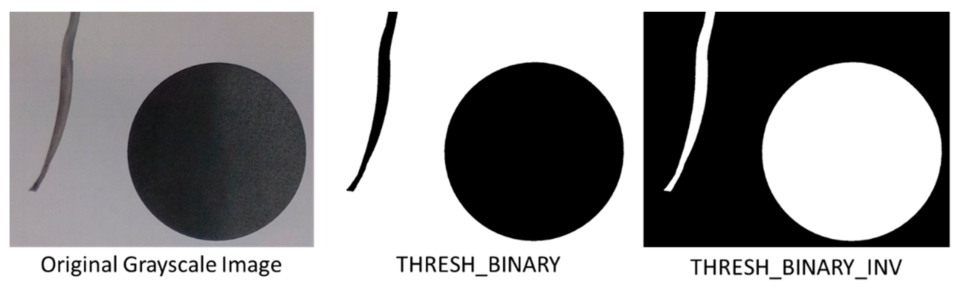
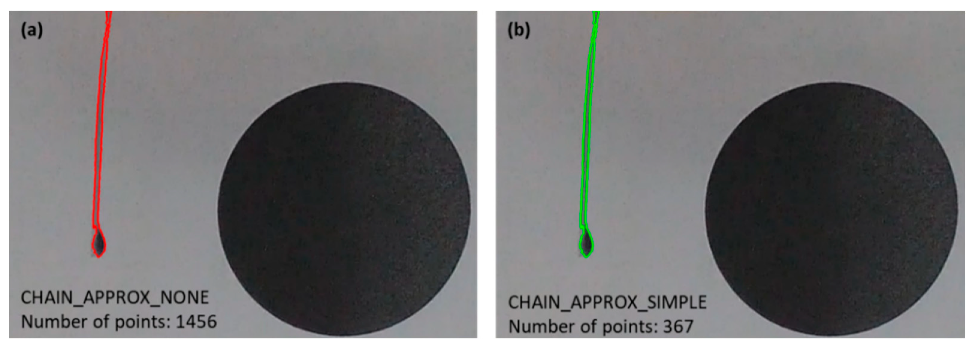
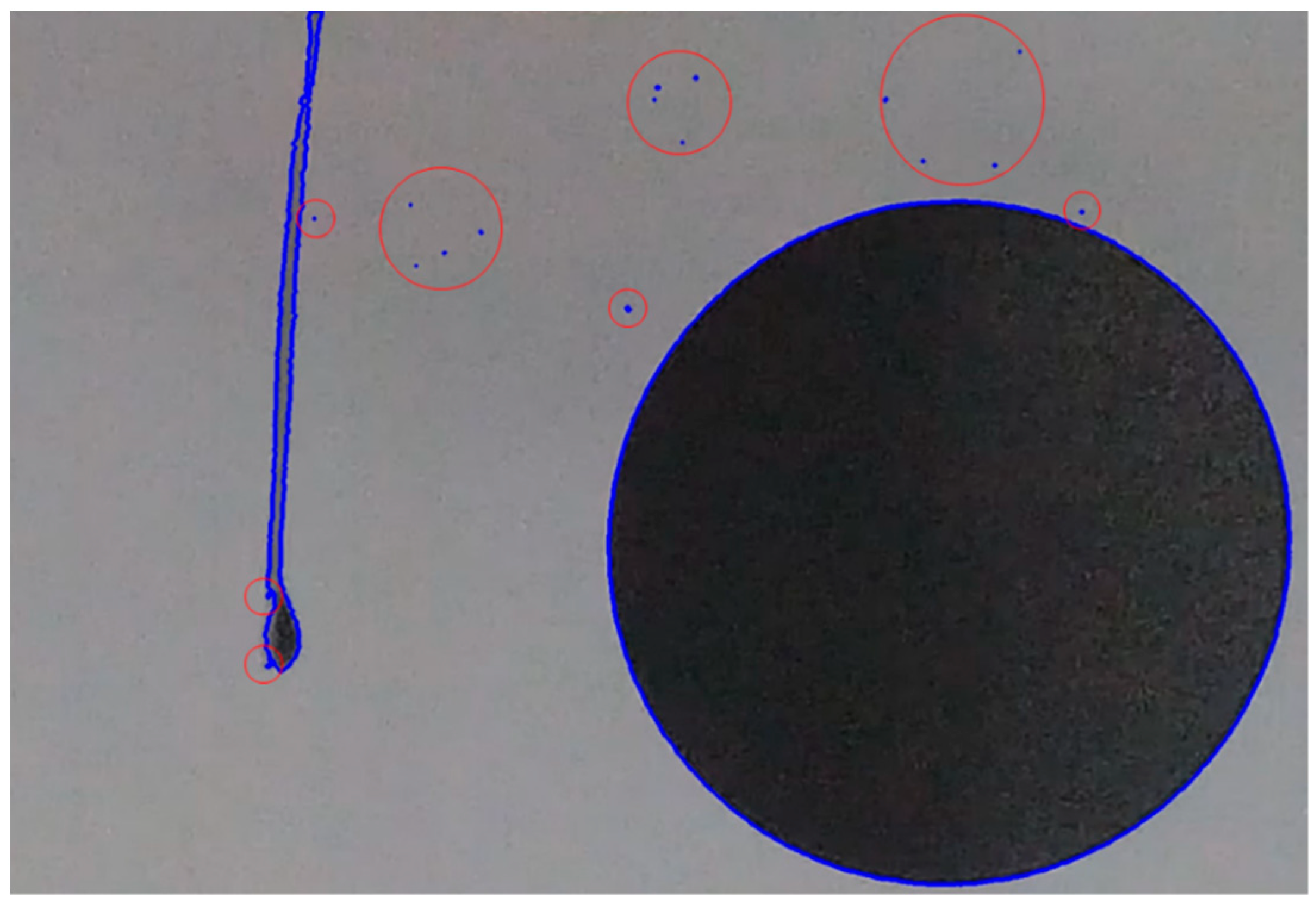
2.2. Contour Detection of IPMC

Unlike the human brain, computers cannot easily deduce an apple from an orange unless specific criteria have been defined to differentiate between the two e.g., apple is red, orange is orange [19]. Similarly, computers cannot determine which is the IPMC sample in the images unless specific definitions have been made. Utilising the setup as illustrated in Figure 1, the human brain can differentiate between the sample and the background based on several parameters such as colour, object geometry, area and position. To further illustrate this scenario, take an example where the sample will be a silver-blackish colour with a somewhat rectangular geometry and a small area positioned near the middle of the image. These parameters need to be translated and defined for a computer program to understand [19]. However, not all the parameters need to be defined. The only parameters needed are the ones unique and identifiable only to the object being detected.

In the case of platinum-coated Nafion IPMCs, the most identifiable parameter of the sample would be its silver-blackish colour. Against a light backdrop, the dark gradient would contrast well with the light background. Regarding contour detection, more accuracy will be obtained using binary images. Thus, a suitable method to binarize the image would be thresholding. Thresholding takes a grayscale image and turns it bitonal [20]. In grayscale images, the tonal shades of gray are numbered from 0 to 255, with 0 being black and 255 being white. A threshold value is set, and if the pixel intensity is above this value, it is set to white (255). If the pixel intensity is below the threshold, it is set to black (0).

In the OpenCV library, the thresholding function requires three input parameters excluding the image: threshold value, maximum value and thresholding type [20]. Maximum value in this case is the maximum grayscale value desired. If the pixel intensity is above the set threshold, it does not have to necessarily be set to white (255) but set to another value less than 255. With regards to thresholding type, several options are available [20]. In this application, the author deems the following two types to be relevant; THRESH_BINARY and THRESH_BINARY_INV. Mathematical notations for the two types are given in

Table 1. Mathematical notations for the two types of thresholding.

Enumerator	Mathematical Notation
THRESH_BINARY	$dst\left(x,y\right)=\{\begin{array}{c}maxval if src\left(x,y\right)>thresh\\ 0 otherwise \end{array}$
THRESH_BINARY_INV	$dst\left(x,y\right)=\{\begin{array}{c} 0 if src\left(x,y\right)>thresh\\ maxval otherwise \end{array}$

.

The function THRESH_BINARY is the common type of thresholding whereby pixel values are set to the maximum value if they exceed the set threshold and set to 0 if they are below it. Alternatively, THRESH_BINARY_INV is the inverted version of the prior type. If pixel intensity exceeds threshold, its value is set to 0, and if it is below that, it is set to the maximum value. The visual difference between these two types can be seen in Figure 9.

It should be noted that to obtain a good thresholding result, Gaussian blur (also known as Gaussian smoothing) must be applied to the grayscale image to reduce noise [12,21]. In this study, THRESH_BINARY_INV was used to isolate the outline of the sample with the maximum value set to 255. The threshold value can vary from sample to sample, since the IPMC sample is not a solid black or silver colour. It can be considered as a gradient, with regions of deep black, gray and silver colours. Thus, trial-and-error is needed to determine the threshold value. Fortunately, the grayish-black IPMC contrasts well with the white background. Referring to the grayscale tonal range in Figure 10, the threshold value should be in the range of 100 to 170, depending on the colour distribution of the samples. The threshold value should be set to the lightest region of the sample.

A convenient approach to this is through an image manipulation software like GIMP [23]. Sample a frame of the IPMC sample, convert it to grayscale and apply a 5 × 5 Gaussian blur. Using the ‘Colour Picker Tool’ function, highlight the lightest region of the IPMC. This should output the colour of the region in Red–Green–Blue (RGB) values which can then be converted to the grayscale range and be set as the threshold value.

Contour detection is done by the cv2.findContours function in OpenCV [24]. The function has the following input parameters: image, mode, method, contours, hierarchy and offset. In this study, only two parameters, mode and method, are of focus. ‘Mode’ refers to the contour retrieval mode, and ‘method’ is the contour approximation method. There are several contour retrieval modes, each differing from the other in terms of which contours are retrieved and the contour hierarchy established. In a controlled setting with a fixed camera setup, consistent lighting and no shadows, using contour retrieval mode RETR_LIST is adequate. This mode retrieves all the contours without establishing any hierarchy between them.

The method parameter on the other hand determines which contour points are stored. Taking an image of a line for example, not all the points are needed to establish its contour—only the two end points. Similarly, only the four corner points of a rectangle are needed to establish its contour. In OpenCV there are four contour approximation methods: CHAIN_APPROX_NONE, CHAIN_APPROX_SIMPLE, CHAIN_APPROX_TC89_L1 and CHAIN_APPROX_TC89_KCOS. The latter two methods are concerning the Teh-Chin chain approximation algorithm [25]. The first two methods are deemed adequate for this application by the authors, with CHAIN_APPROX_NONE storing all the contour points and CHAIN_APPROX_SIMPLE compressing horizontal, vertical, and diagonal segments leaving only the end points. No differences were found in the contour detection of the sample between the two methods, as shown in Figure 11. The number of contour points stored in CHAIN_APPROX_SIMPLE is significantly less than CHAIN_APPROX_NONE. Thus, the prior approximation method is utilised since it uses less memory and reduces processing time [26].

With the input parameters set, the contours can be extracted for further computing. To check whether all the contours are correctly identified, the function cv2.drawContours can be used to draw extracted contours on the original image.

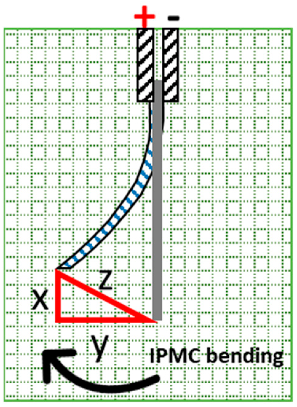
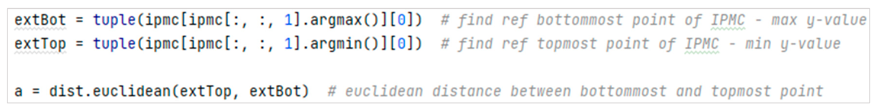
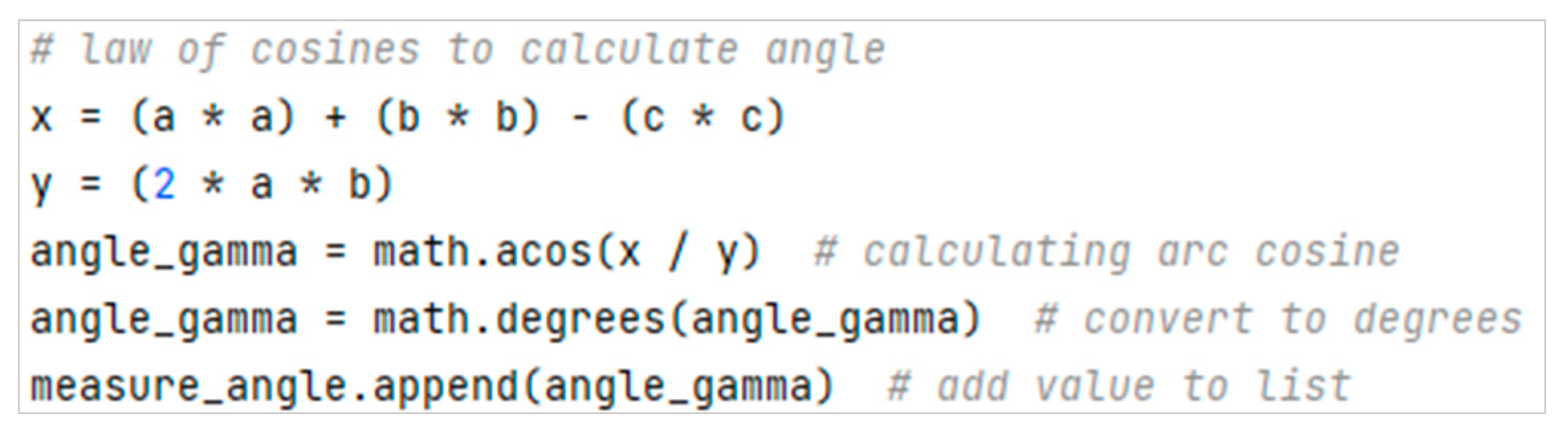
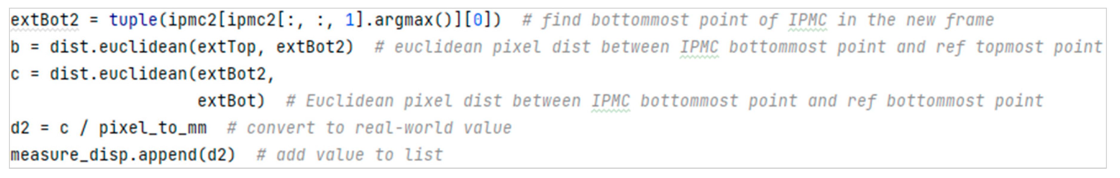
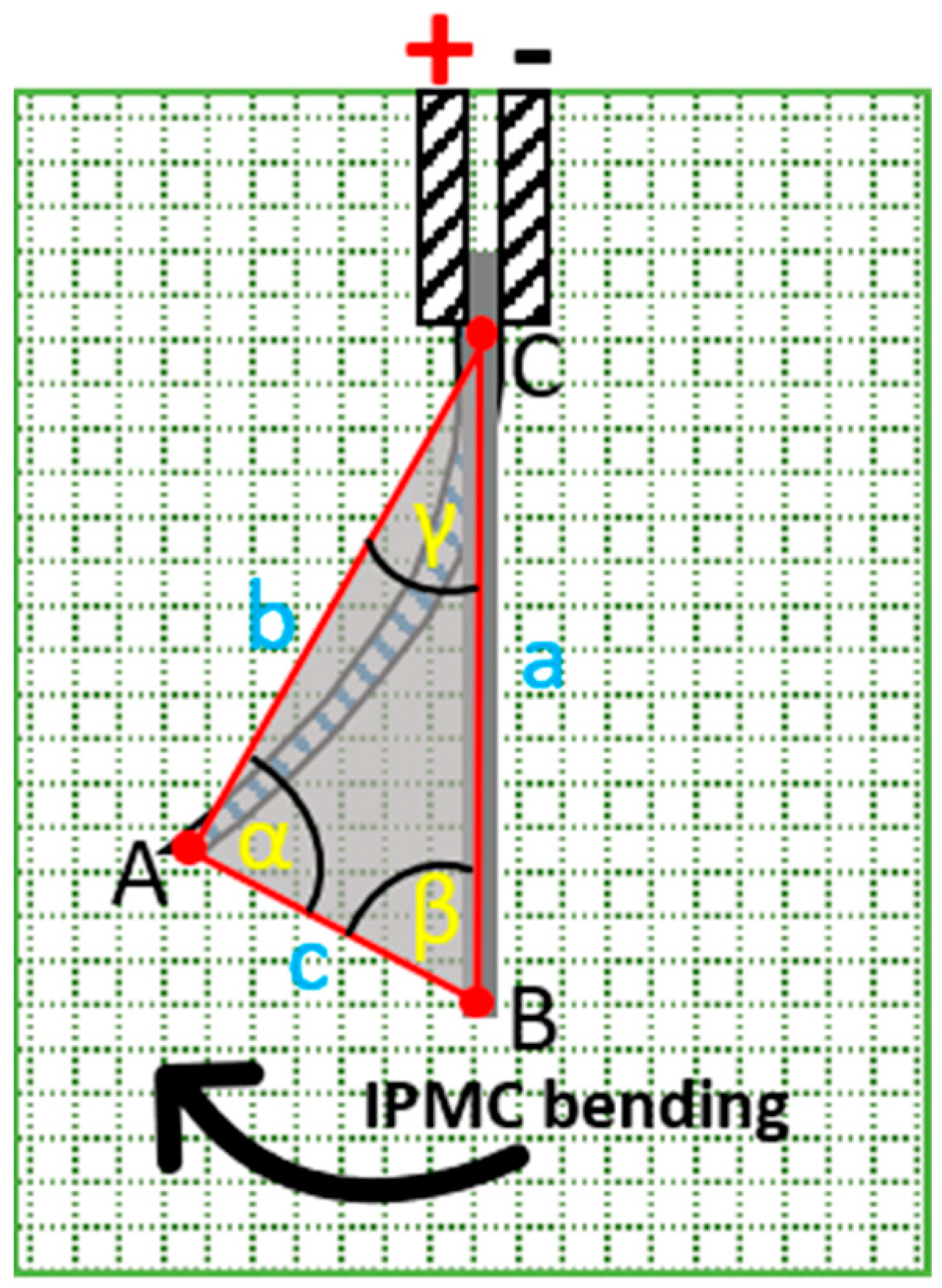
2.3. Contour Extreme Points: Finding Displacement and Bending Angle

As IPMC displaces under the influence of voltage, the tip of the IPMC will always be at the end—an extreme point of the contour. OpenCV accesses pixels through a Cartesian coordinate system, represented as 2-tuples (x,y), with the origin (0,0) being at the top-left corner of the image [27]. The values in the x and y axes increase positively as you move diagonally across the image. Deducing the tip of the IPMC to always have a maximum y-value, in the code, this point can be located using the argmax() function, specifying it for the y-value of the contour points [28]. This can be used to find the tip point in every frame and calculate the distance between those points to get the displacement values. A linear displacement method with reference to the initial frame is utilised, similar to the method described in Figure 2. It should be noted that the bending is more accurately described by the arc length between two IPMC tips. However, due to the non-uniform curvature and off-axis deformations of IPMCs [14], the bending centre changes. Calculating the arc length is difficult as the pivot point and radius (effective length of the sample) change. Tsiakmakis et al. proposed a method to utilise the arc length calculation by detecting several points on the IPMC to find the radius and using the intersection of lines through those points to find the bending centre [11,12]. However, no details were given as to how those points were detected by the algorithm.

The IPMC tips are also used to calculate bending angle. One of the many ways to determine the bending angle in this case is by employing the Law of Cosines, a law which relates the lengths of the triangle to the cosine of the angles. Such relations are given in Equations (1)–(3). Relating the triangle to the IPMC sample in Figure 12, points A and B are the tips of the IPMC as displacement occurs. The angle of interest, γ, is the bending angle. Point C is a reference point—the topmost point of the IPMC contour. This point can be identified using the argmin() function, which finds the minimum value, and specifying it for the y-value of the contour points. Having detected all three points of the triangle, Equation (1) can be used to find bending angle γ. In this application, points B and C are identified in the initial frame and are kept constant as they serve as reference points for measurement. Only point A changes with each subsequent frame. In the code, the Math module was employed to use the arccosine function (math.acos()) to find the angle. Note that this function outputs the angle in radians. Conversion from radians to degrees can be done using the math.degrees() function.

$$c^2=a^2+b^2-2ab\cos \gamma$$

(1)

$$a^2=b^2+c^2-2bc\cos \alpha$$

(2)

$$b^2=a^2+c^2-2ac\cos \beta$$

(3)

2.4. Converting Pixel Distance to Real-World Units

A difficulty encountered with vision systems employed to measure distances or sizes is how one would translate pixels values to real-world units like centimetres or inches. As described in [11], the relationship between the pixel size and real-world units must be defined. A reference object of known dimensions present in the image is needed. In this application, a black circle of diameter 50 mm is printed onto the background. The idea is to find the pixel diameter of the circle, and divide that by the actual diameter in mm, yielding a pixel-to-millimetre (PMM) ratio which can be used to convert pixel values to millimetres. The pixel diameter of the circle can be identified by finding the distance between the leftmost and rightmost points of the circle. The leftmost point will have a minimum x-value, whereas the rightmost point will have a maximum. Both argmin() and argmax() functions, specified to the x-value of the circle contour points, can be utilised to find the extreme points [28].

2.5. Lights, Camera and Actuation

Coding described in the previous sections will only be effective if paired with an appropriate camera configuration. Effectiveness of the vision system is, up to a point, limited by the quality of the input images. This section will be discussing in depth the suitable camera setup for this specific application. Four main camera settings should be focused on: resolution, frame rate, shutter speed and field of view.

‘Resolution’ refers to the number of pixels in one frame. Clarity and level of detail in a video recording or image depends on the resolution. A higher pixel count equals better image quality [30]. Standard resolutions range from 640 × 360 (360 p) up to 7680 × 4320 (8 K) [31]. Increasing resolution means more detail in the image, but also increased file size. Based on the findings in this study, the authors recommend a minimum resolution of 1280 × 720 (720 p) for a clear and detailed image. A good compromise between resolution and file size would be shooting at 1920 × 1080 (1080 p) resolution.

Video is just a series of photos captured consecutively at a relatively high rate. Frame rate, measured in frames per second (fps) is how many frames or pictures the camera can capture per second [32]. More frames per second equals a smoother and more detailed representation of the IPMC bending. Movies and television shows, for example, are shot at 30 fps, whereas sporting events involving fast motions are shot at 60 fps or 120 fps. Mid-range smartphones and cameras nowadays offer a shooting range of 60 fps at 1080 p resolution, with higher end products offering filming resolutions of up to 7680 × 4320 (8 K) and 240 fps. High-speed cameras also offer higher fps, but they can be very expensive. For the application of looking at IPMC bending, the authors deem shooting at 50/60 fps to be adequate.

Shutter speed is how long the camera shutter stays open [33]. It is closely related to the concept of motion blur. Motion blur is the apparent light streaks produced by objects in motion. Figure 13 demonstrates an image of a finger being flicked, exhibiting motion blur. This pronounced effect is controlled by the shutter speed of the camera.

A faster shutter speed allows less light to be captured by the camera sensor, and a slower shutter speed keeps the shutter open for a longer time, allowing for more light to be captured [33]. Shutter speed is generally expressed as fractions of a second. Shutter speed values range from 1/2 a second to 1/8000th of a second on some cameras, whilst others can have values up to 30 s. In this instance, 30 s shutter speed is the slowest shutter speed whereas 1/8000th of a second is the fastest shutter speed. It is important to note that with increasing shutter speed, brightness decreases as the camera sensor is exposed to less light. In measuring IPMC displacement, since the bending velocity is not comparable to that of a fast-moving race car, the shutter speed should be less than a thousandth of a second. A simple way to determine the best shutter speed is by doing a simple finger-flicking test. Film a sequence of videos capturing the continuous flicking of a finger. With each video iteration, move up a shutter speed. Go through the videos frame by frame. At the right shutter speed, the frame-by-frame images of the finger will be crisp and clear with no motion blur present.

The final setting is the field of view (FOV) of the camera. Depending on the camera model utilised, some exhibit distortion is caused by the lens used. Optical distortion, also known as lens distortion, occurs due to the optical design of lenses causing straight lines to appear curved [34]. Several types of lens distortions are shown in Figure 14. To accurately capture and calculate IPMC displacement, having no lens distortion is desirable. Some cameras have configurable field of view settings in the menu, whereas other cameras, like digital single-lens reflex (DSLR) cameras, the lenses need to be swapped out for a linear FOV (no lens distortion).

Once camera settings have been optimised, the IPMC bending can be captured. Extracting the frames from the recording can be done several ways. One option is to employ a frame grabber—an electronic device that captures frames from an analogue or digital video signal. This device is usually connected to a camera and a computer. Another option is to extract still frames through software processing of the video. In video editing applications such as Final Cut Pro and VEGAS Pro, there are options to render media as a sequence of still frames in image formats such as JPEG (joint photographic experts group) and PNG (portable network graphics).

With regards to lighting, the aim is to not have shadows appear in the image, as this will mess up contour detection of the IPMC sample and the reference object, affecting measurement accuracy [12]. It is recommended to have a light source illuminating the scene.

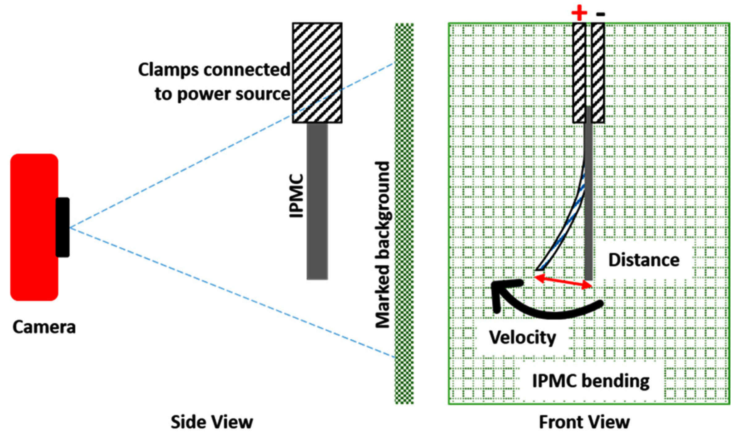
3. Experimental Setup

In order to ascertain the accuracy of the proposed vision system, results from the vision system needed to be compared to results from the manual calculation. Previous literature used a grid background as reference for displacement values. However, with the presence of a reference circle in the frame, the grid background is rendered redundant. Thus, the manual calculation method utilised in this comparison employed the reference circle instead of a grid background. With the help of MB Ruler software [17], the PMM value was determined by dividing the pixel diameter of the circle by 50 mm. The tip-to-tip linear displacement values of the IPMC were then determined and converted to mm using the calculated ratio.

3.1. Camera & Lighting Setup

An Insta360 One R camera mounted with the 4 K wide angle lens with F2.8 aperture was used. This camera model has four distinctive video FOV settings: narrow, linear, wide and ultrawide. From Figure 15, it can be seen that the wide and ultrawide FOVs produce images with barrel distortion. The narrow FOV was chosen.

Resolution was set to 1080 p recording at 50 fps. As mentioned earlier, the finger flick test was used to determine the appropriate shutter speed. The following shutter speeds were tested; 1/100, 1/120, 1/160, 1/200, 1/240, 1/320 and 1/400. Minimal motion blur was detected at 1/320. At 1/400, frames exhibited clear and crisp images with no motion blur present. This was the shutter speed chosen for this study. Several coloured backgrounds were tested for good contrast with the sample; some are shown in Figure 16. A white background was chosen.

A JOBY Beamo 12” ring light was used as a light source. The ring light has three colour temperature modes—3000 K, 4000 K and 5600 K—each with ten adjustable intensity levels. Colour temperature mode 5600 K was used, at max intensity level. In the sequence of setting up the lighting, it was very difficult to completely remove shadows when the IPMC sample is close to the background. More light sources could be added to help minimise the shadows. However, a more effective method would be to place the sample some distance away from the background, allowing light to reach the previously overshadowed regions. The sample was placed 4 mm away from the background, and the camera was placed 20 mm away from the sample to keep it in focus. The sample, camera and background were all placed parallel to each other.

3.2. Sample Preparation

An IPMC sample with the dimensions 10 × 50 mm was prepared according to methods prescribed in the literature [35,36]. Nafion-117, obtained from Ion Power GmbH and tetraammineplatinum(II) chloride hydrate (98%), obtained from Sigma-Aldrich was used. The IPMC was soaked in a 2 M lithium chloride solution. Reducing agents and other miscellaneous chemicals were obtained from Fisher Scientific.

3.3. Clamping, Voltage and Frame Extraction

Samples were clamped using a cloth pin with the ends wrapped in strips of aluminium foil. One strip was connected to the positive side of the voltage regulator, the other to the negative side. Initially, 9 V were applied to the IPMC for approximately 5 s. The first 3 s of the bending video were taken and cropped using Vegas Pro 14 to only show the sample and the reference circle. The footage was then exported as images in PNG format, with 3 s of video shot at 50 fps resulting in 150 images/frames. The threshold value was set to 120 and the maximum value was set to 255.

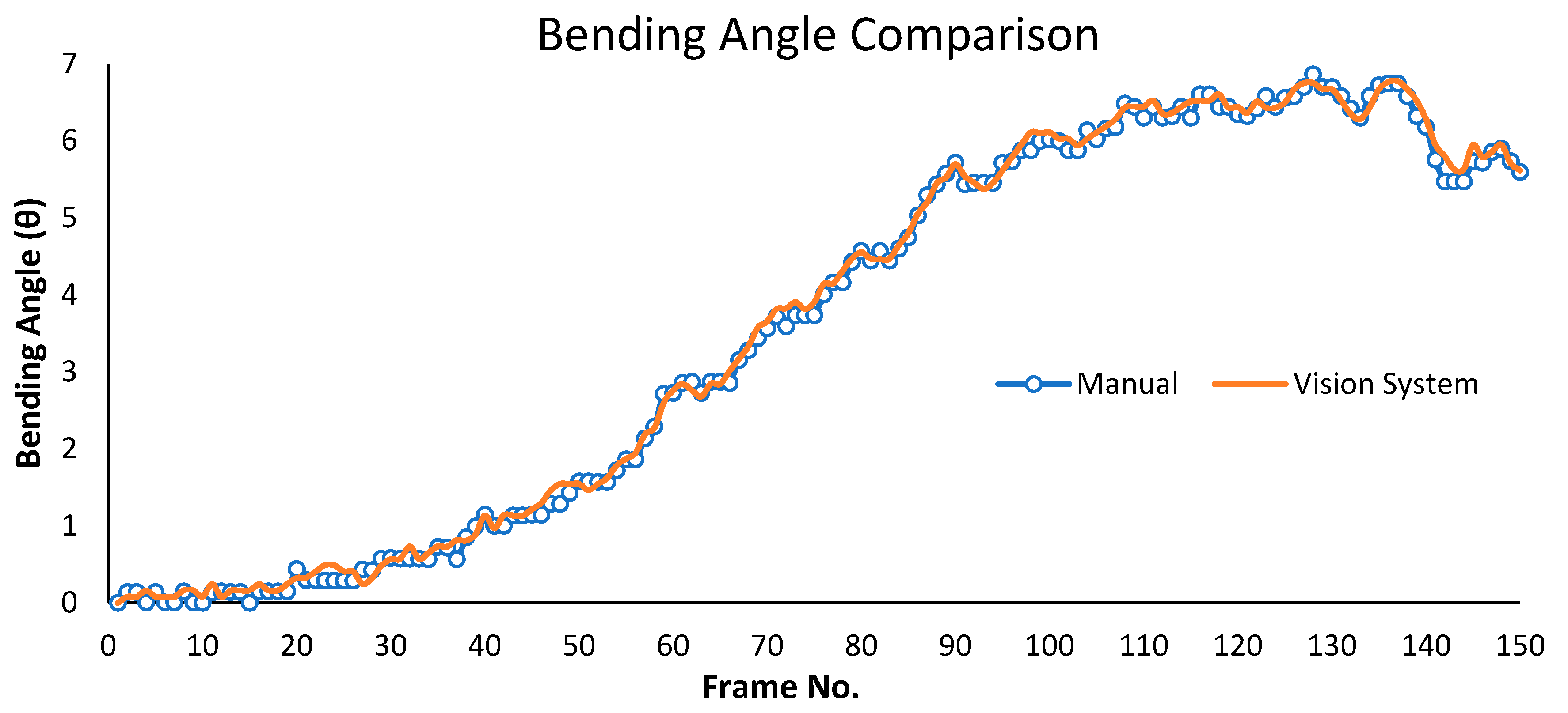
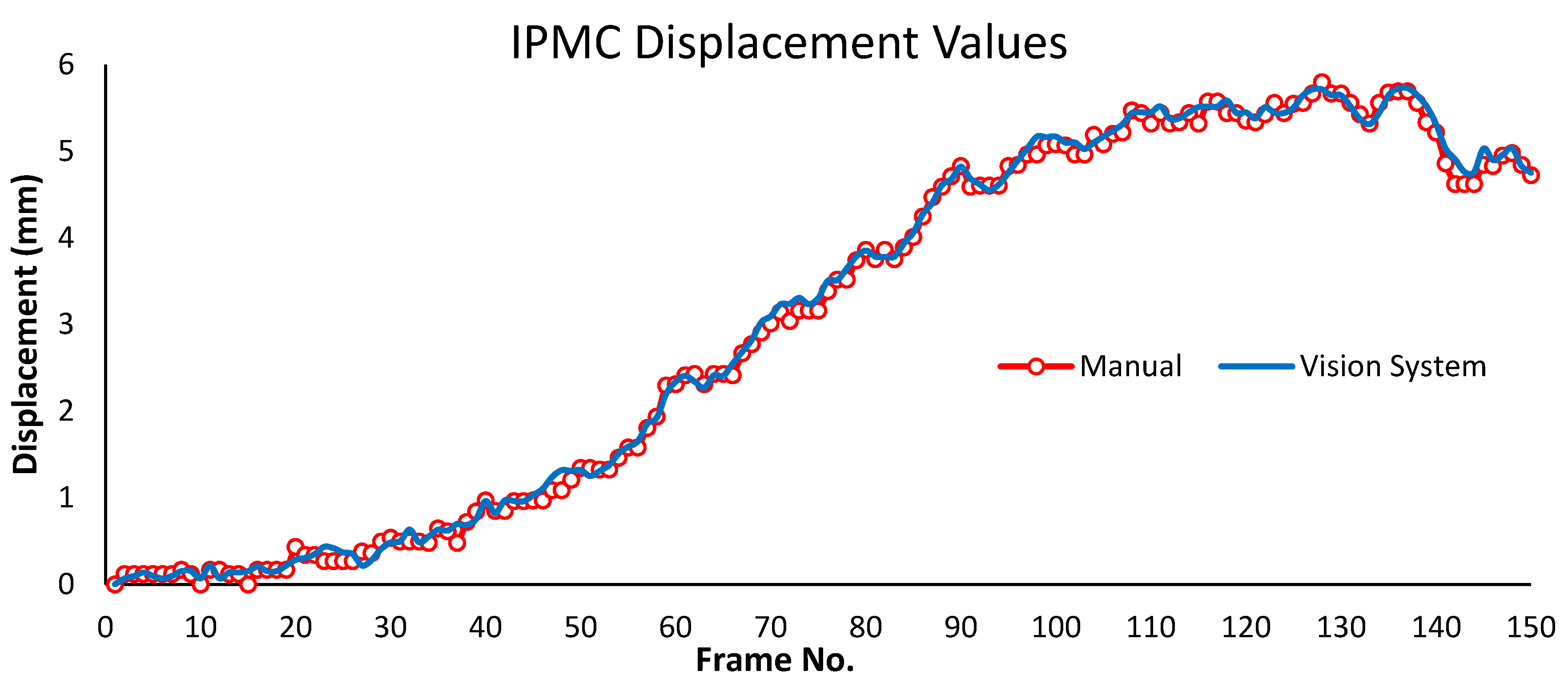
4. Results and Discussion

Several runs of the coding with IPMC bending video proved it was difficult to only isolate the contours of the sample and the reference circle. In Figure 17, circled in red, are the detected small contours, consisting of image noise and small dust particles in the air and on the camera lens. Contours near the reference circle are tiny ink splashes from the printer—hard to notice with the naked eye. Several small contours detected on the sample were due to the non-uniform colour distribution of the platinum-coated Nafion surface. Some of these can be eliminated by changing the threshold value, but this results in the contours of the sample and the reference circle not being perfectly detected.

The first iteration of the code saw the sample and reference circle being distinguished from each other as having minimum and maximum contour areas, respectively. Having other contours present besides the two required would render the code futile. Accounting for this, the improved code sorted contours by their areas. In this setup, the reference circle with a diameter of 50 mm was configured to always have both more contour area than the sample and the maximum contour area in the frame. The sample will have the second largest contour area. Contours were sorted by their areas using the sorted() function, setting the key as contour area. By default, this function sorts the areas in ascending order, from smallest to largest contour area. Areas were sorted in descending order by adding reverse=True in the function [37]. Reference circle contour was then set to the largest contour area, whereas the sample was set to the second largest. Displacement results from the improved vision system and the manual calculation method are shown in Figure 18.

Visually inspecting the displacements values obtained from both methods, the results generally follow the same trend with no significant deviations between one another. Deviations in results between the manual method and the proposed vision system can statistically be calculated using mean absolute error (MAE) and root mean squared error (RMSE). Calculated values of MAE and RMSE are 0.068080668 and 0.088160652, respectively. A similar trend can be seen in bending angle values, as shown in Figure 19.

The calculated values of MAE and RMSE for bending angle are 0.081544205 and 0.103880163, respectively. Low values of MAE and RMSE signify agreeable results between both methods. It can be concluded that the vision system proposed can accurately approximate the displacement and bending angle values of Nafion-based ionic polymer–metal composites.

Limitations and Recommendations

The proposed vision system has several limitations—one of them involving the detection of the IPMC tip. The system detects the IPMC tip by finding the contour point with a maximum y-coordinate. Assuming a rigid, straight IPMC sample initially positioned vertically, this method will not work once the sample is in a horizontal position, i.e., when the bending angle equals 90°. However, in reality, some samples will have a slight curvature to them. In these instances, the detection method will cease to work at bending angles less than 90°. Furthermore, the proposed system only approximates the linear displacement of IPMCs, which can be quite accurate for small movements, up to about half the length of the IPMC [12]. However, as mentioned earlier, the bending is more accurately described by the arc length between points of the IPMC tip.

This proposed vision system requires specific conditions for the measurements to be accurate, such as having a good contrast between the sample and the background, having no shadows present and camera configurations with specific settings. These factors need to be adjusted depending on the sample, since colour uniformity between samples might differ. Several pre-processing (crop video, extract frames, feed images to programme) steps are also required to obtain displacement values. Results are not real-time. The system can be more streamlined by automating these processes, cutting down the need for human intervention. An example would be the setup presented in [12].

Regarding lens distortion, another avenue to minimize the effects is through software correction. OpenCV has an inbuilt function for camera calibration. Through analysing sets of checkerboard images, the intrinsic and extrinsic properties of the camera can be calculated and used to calibrate images accordingly [38].

5. Conclusions

A computer vision system was proposed to measure the displacement and bending angle of ionic polymer-metal composite (IPMC) utilising Python in conjunction with OpenCV. Coding functions and the mathematical formulas used were described. IPMC contour detection was discussed in detail. Extreme points detection of the IPMC contour was used to obtain the tip-to-tip displacement values. Appropriate camera settings were discussed, mainly focusing on four settings: resolution, frame rate, shutter speed and field of view. A linear displacement calculation method was used for this study. Measurements generated from the vision system were experimentally compared to approximated values via the manual calculation method. Good agreement was found between the results produced by the two methods. However, the system is not without its limitations. Main issues include cessation of the system as it approaches close to the maximum bending angle of 90° and requiring specific conditions for effective detection of IPMCs. Furthermore, the linear displacement calculation method used in this study cannot accurately describe the IPMC bending as compared to the arc length between IPMC tips. Due to the off-axis deformation and non-uniform curvature of IPMCs, the later calculation method cannot be used in this vision system unless an effective method of detecting the bending centre has been developed. The authors conclude that the proposed vision system can accurately approximate the displacement and bending angle of IPMCs. A GitHub link to the open-access code can be found in the Supplementary Materials section.

References

1. Bar-Cohen, Y.; Cardoso, V.F.; Ribeiro, C.; Lanceros-Méndez, S. Chapter 8—Electroactive Polymers as Actuators. In Advanced Piezoelectric Materials, 2nd ed.; Uchino, K., Ed.; Woodhead Publishing: Sawston, UK, 2017; pp. 319–352. [Google Scholar] [CrossRef]
2. He, C.; Gu, Y.; Zhang, J.; Ma, L.; Yan, M.; Mou, J.; Ren, Y. Preparation and Modification Technology Analysis of Ionic Polymer-Metal Composites (IPMCs). Int. J. Mol. Sci. 2022, 23, 3522. [Google Scholar] [CrossRef] [PubMed]
3. He, Q.; Yin, G.; Vokoun, D.; Shen, Q.; Lu, J.; Liu, X.; Xu, X.; Yu, M.; Dai, Z. Review on Improvement, Modeling, and Application of Ionic Polymer Metal Composite Artificial Muscle. J. Bionic Eng. 2022, 19, 279–298. [Google Scholar] [CrossRef]
4. Luqman, M.; Shaikh, H.; Anis, A.; Al-Zahrani, S.M.; Hamidi, A. Platinum-coated silicotungstic acid-sulfonated polyvinyl alcohol-polyaniline based hybrid ionic polymer metal composite membrane for bending actuation applications. Sci. Rep. 2022, 12, 4467. [Google Scholar] [CrossRef]
5. Yılmaz, O.C.; Sen, I.; Gurses, B.O.; Ozdemir, O.; Cetin, L.; Sarıkanat, M.; Seki, Y.; Sever, K.; Altinkaya, E. The effect of gold electrode thicknesses on electromechanical performance of Nafion-based Ionic Polymer Metal Composite actuators. Compos. Part B Eng. 2019, 165, 747–753. [Google Scholar] [CrossRef]
6. Asaka, K.; Oguro, K.; Nishimura, Y.; Mizuhata, M.; Takenaka, H. Bending of Polyelectrolyte Membrane–Platinum Composites by Electric Stimuli I. Response Characteristics to Various Waveforms. Polym. J. 1995, 27, 436–440. [Google Scholar] [CrossRef] [Green Version]
7. Asaka, K.; Oguro, K. Bending of polyelectrolyte membrane platinum composites by electric stimuli: Part II. Response kinetics. J. Electroanal. Chem. 2000, 480, 186–198. [Google Scholar] [CrossRef]
8. Asaka, K.; Oguro, K. Bending of polyelectrolyte membrane-platinum composite by electric stimuli. III: Self-oscillation. Electrochim. Acta 2000, 45, 4517–4523. [Google Scholar] [CrossRef]
9. Tripathi, A.; Chattopadhyay, B.; Das, S. Actuation behavior of ionic polymer-metal composite based actuator in blood analogue fluid environment. Polym.-Plast. Technol. Mater. 2020, 59, 1268–1276. [Google Scholar] [CrossRef]
10. Yang, L.; Zhang, D.; Zhang, X.; Tian, A.; Ding, Y. “Surface roughening of Nafion membranes using different route planning for IPMCs. Int. J. Smart Nano Mater. 2020, 11, 117–128. [Google Scholar] [CrossRef]
11. Tsiakmakis, K.; Brufau, J.; Puig-Vidal, M.; Laopoulos, T. Measuring Motion Parameters of Ionic Polymer-Metal Composites (IPMC) Actuators with a CCD Camera. In Proceedings of the 2007 IEEE Instrumentation Measurement Technology Conference IMTC, Warsaw, Poland, 1–3 May 2007; pp. 1–6. [Google Scholar] [CrossRef]
12. Tsiakmakis, K.; Brufau-Penella, J.; Puig-Vidal, M.; Laopoulos, T. A Camera Based Method for the Measurement of Motion Parameters of IPMC Actuators. IEEE Trans. Instrum. Meas. 2009, 58, 2626–2633. [Google Scholar] [CrossRef]
13. Bar-Cohen, Y.; Bao, X.; Sherrit, S.; Lih, S.-S. Characterization of the Electromechanical Properties of Ionomeric Polymer-Metal Composite (IPMC). Proc. SPIE—Int. Soc. Opt. Eng. 2002, 4695, 286–293. [Google Scholar] [CrossRef]
14. Bar-Cohen, Y.; Sherrit, S. Characterization of the Electromechanical Properties of EAP materials. Proc. SPIE—Int. Soc. Opt. Eng. 2001, 4329, 319–327. [Google Scholar] [CrossRef] [Green Version]
15. Li, S.; Yip, J. Characterization and Actuation of Ionic Polymer Metal Composites with Various Thicknesses and Lengths. Polymers 2019, 11, 91. [Google Scholar] [CrossRef] [PubMed] [Green Version]
16. Nemat-Nasser, S.; Wu, Y. Comparative experimental study of ionic polymer–metal composites with different backbone ionomers and in various cation forms. J. Appl. Phys. 2003, 93, 5255. [Google Scholar] [CrossRef] [Green Version]
17. Ma, S.; Zhang, Y.; Liang, Y.; Ren, L.; Tian, W.; Ren, L. High-Performance Ionic-Polymer–Metal Composite: Toward Large-Deformation Fast-Response Artificial Muscles. Adv. Funct. Mater. 2020, 30, 1908508. [Google Scholar] [CrossRef]
18. Pulli, K.; Baksheev, A.; Kornyakov, K.; Eruhimov, V. Realtime Computer Vision with OpenCV: Mobile computer-vision technology will soon become as ubiquitous as touch interfaces. Queue 2012, 10, 40–56. [Google Scholar] [CrossRef]
19. Brownlee, J. Deep Learning for Computer Vision: Image Classification, Object Detection, and Face Recognition in Python; Machine Learning Mastery: San Juan, Puerto Rico, 2019. [Google Scholar]
20. Rosebrock, A. OpenCV Thresholding (cv2.threshold). PyImageSearch. 2021. Available online: https://www.pyimagesearch.com/2021/04/28/opencv-thresholding-cv2-threshold/ (accessed on 4 May 2022).
21. Blackledge, J.M. Digital Image Processing: Mathematical and Computational Methods; Woodhead Publishing: Oxford, UK, 2005. [Google Scholar]
22. Joram, N. Converting RGB image to the Grayscale image in Java. Javarevisited. 2021. Available online: https://medium.com/javarevisited/converting-rgb-image-to-the-grayscale-image-in-java-9e1edc5bd6e7 (accessed on 8 April 2022).
23. Kimball, S.; Mattis, P. GIMP. 2021. Available online: https://www.gimp.org/ (accessed on 11 April 2022).
24. Chakraborty, D. OpenCV Contour Approximation. PyImageSearch. 2021. Available online: https://www.pyimagesearch.com/2021/10/06/opencv-contour-approximation/ (accessed on 6 May 2022).
25. Teh, C.-H.; Chin, R.T. On the detection of dominant points on digital curves. IEEE Trans. Pattern Anal. Mach. Intell. 1989, 11, 859–872. [Google Scholar] [CrossRef] [Green Version]
26. Mallick, S. Contour Detection using OpenCV (Python/C++). LearnOpenCV. 2021. Available online: https://learnopencv.com/contour-detection-using-opencv-python-c/ (accessed on 12 April 2022).
27. Rosebrock, A. OpenCV Getting and Setting Pixels. PyImageSearch. 2021. Available online: https://www.pyimagesearch.com/2021/01/20/opencv-getting-and-setting-pixels/ (accessed on 3 May 2022).
28. Rosebrock, A. Finding extreme points in contours with OpenCV. PyImageSearch. 2016. Available online: https://www.pyimagesearch.com/2016/04/11/finding-extreme-points-in-contours-with-opencv/ (accessed on 5 May 2022).
29. Weisman, D. Triangle with Notations for Sides and Angles. 2006. Available online: https://commons.wikimedia.org/wiki/File:Triangle_with_notations_2.svg (accessed on 13 April 2022).
30. Catoy, K. The Basics of Video Resolution. Video4Change. 2020. Available online: https://video4change.org/the-basics-of-video-resolution/ (accessed on 4 May 2022).
31. Surana, N. A Complete List of Video Resolutions and their Pixel Size. Typito. 2020. Available online: https://typito.com/blog/video-resolutions/ (accessed on 6 May 2022).
32. Kurniawan, M.; Hara, H. A Beginner’s guide to frame rates in films | Adobe. Adobe. 2020. Available online: https://www.adobe.com/ie/creativecloud/video/discover/frame-rate.html (accessed on 17 May 2022).
33. Mansurov, N. Understanding Shutter Speed for Beginners—Photography Basics. Photography Life. 2018. Available online: https://photographylife.com/what-is-shutter-speed-in-photography (accessed on 4 May 2022).
34. Gray, D. Distortion 101—Lens vs. Perspective. Drew Gray Photography—Interior/Architectural/Landscaping. 2014. Available online: http://www.drewgrayphoto.com/learn/distortion101 (accessed on 25 February 2022).
35. Kim, K.J.; Shahinpoor, M. Ionic polymer metal composites: II. Manufacturing techniques. Smart Mater. Struct. 2003, 12, 65–79. [Google Scholar] [CrossRef]
36. Yang, L.; Zhang, D.; Wang, H.; Zhang, X. Actuation Modeling of Ionic–Polymer Metal Composite Actuators Using Micromechanics Approach. Adv. Eng. Mater. 2020, 22, 2000537. [Google Scholar] [CrossRef]
37. Rosebrock, A. Sorting Contours using Python and OpenCV. PyImageSearch. 2015. Available online: https://www.pyimagesearch.com/2015/04/20/sorting-contours-using-python-and-opencv/ (accessed on 4 May 2022).
38. Sadekar, K.; Mallick, S. Camera Calibration using OpenCV | LearnOpenCV #. LearnOpenCV. 2020. Available online: https://learnopencv.com/camera-calibration-using-opencv/ (accessed on 17 May 2022).
Figure 1. Digital camera setup to measure IPMC displacement.
Applsci 12 06744 g001
Figure 2. Calculating IPMC bending displacement.
Applsci 12 06744 g002
Figure 3. Flow chart of the proposed progression of the vision system.
Applsci 12 06744 g003
Figure 4. Importing necessary modules.
Applsci 12 06744 g004
Figure 5. Use of OpenCV to load, manipulate and analyse image.
Applsci 12 06744 g005
Figure 6. Calculating the Euclidean distance between points.
Applsci 12 06744 g006
Figure 7. Lines 63 to 68 of the code.
Applsci 12 06744 g007
Figure 8. Calculation of the bending angle using the Cosine Law.
Applsci 12 06744 g008
Figure 9. Visual comparison between the original image and the two thresholding types.
Applsci 12 06744 g009
Figure 10. Grayscale tonal range from 0 to 255 [22].
Applsci 12 06744 g010
Figure 11. Sample contour approximation using (a) CHAIN_APPROX_NONE and (b) CHAIN_APPROX_SIMPLE.
Applsci 12 06744 g011
Figure 12. Relating triangle with sides a, b, c and angles α, β, γ to the IPMC setup [29].
Applsci 12 06744 g012
Figure 13. Flicked finger exhibiting motion blur.
Applsci 12 06744 g013
Figure 14. Types of lens distortion [34].
Applsci 12 06744 g014
Figure 15. Insta360 One R FOV options.
Applsci 12 06744 g015
Figure 16. Several coloured backgrounds tested for good contrast with the sample.
Applsci 12 06744 g016
Figure 17. Detection of multiple contours.
Applsci 12 06744 g017
Figure 18. IPMC displacement values obtained from manual calculation and vision system.
Applsci 12 06744 g018
Figure 19. IPMC bending angle values obtained from manual calculation and vision system.
Applsci 12 06744 g019