Determination of Landslide Displacement Warning Thresholds by Applying DBA-LSTM and Numerical Simulation Algorithms

Abstract

Numerical simulation has emerged as a powerful technique for landslide failure mechanism analysis and accurate stability assessment. However, due to the bias of simplified numerical models and the uncertainty of geomechanical parameters, simulation results often differ greatly from the actual situation. Therefore, in order to ensure the accuracy and rationality of numerical simulation results, and to improve landslide hazard warning capability, techniques and methods such as displacement back-analysis, machine learning, and numerical simulation are combined to create a novel landslide warning method based on DBA-LSTM (displacement back-analysis based on long short-term memory networks), and a numerical simulation algorithm is proposed, i.e., the DBA-LSTM algorithm is used to invert the equivalent physical and mechanical parameters of the numerical model, and the modified numerical model is used for stability analysis and failure simulation. Taking the Shangtan landslide as an example, the deformation mechanism of the landslide was analyzed based on the field monitoring data, and subsequently, the superiority of the DBA-LSTM algorithm was verified by comparing it with DBA-BPNN (displacement back-analysis based on back-propagation neural network); finally, the stability of the landslide was analyzed and evaluated a posteriori using the warning threshold calculated by the proposed method. The analytical results show that the displacement back-analysis based on the machine learning (DBA-ML) algorithm can achieve more than 95% accuracy, and the deep learning algorithm exemplified by LSTM had higher accuracy compared to the classical BPNN algorithm, meaning that it can be used to further improve the existing intelligent inversion theory and method. The proposed method calculates the landslide’s factor of safety (FOS) before the accelerated deformation to be 1.38 and predicts that the landslide is in a metastable state after accelerated deformation rather than in failure. Compared to traditional empirical warning models, our method can avoid false warnings and can provide a new reference for research on landslide hazard warnings.

1. Introduction

With the expansion of human activities and the intensification of global climate change, landslide geological hazards are occurring with increasing frequency, causing serious economic losses and casualties. China is one of the regions with the highest number of landslide incidents, and to date, thousands of landslide hazards still occur annually, causing hundreds of deaths and billions of USD (United States dollar) of economic losses, and the hazard prevention and mitigation situation remains severe [1].

Deformation monitoring is an essential means for the active prevention and control of landslide hazards, and with the rapid development of computer technology and geomatics science and technology, novel monitoring technologies such as GNSS, InSAR, and UAV vision have made positive contributions to landslide hazard monitoring and early warning systems [2,3,4]. Generally, InSAR and UAV are employed for landslide early identification and detection over large areas, because of their high spatial resolutions. The authors of [5] investigated the spatial and temporal evolution characteristics of a landslide before and after damage with InSAR, UAV, and remote sensing, and found that InSAR and remote sensing could be used for the early identification of unstable slopes. In [6], GB-InSAR was used to monitor the deformation of talus slopes during excavation, and real-time dynamic landslide warning during excavation was achieved by calculating the change rate of the cross-section of the equidistant body of the slope. Landslide interior monitoring also plays a significant role in supporting the development of slope stability models [7,8]. Study [9] demonstrated the significance of temporal resolution in capturing landslide deformation behavior, and found that the tilt meter and AEWG (acoustic emission monitoring using active waveguides) both captured all phases of the activation motion with sufficient temporal resolution. Study [10] found that the combined approach with the tilt meter and rain gauge can reduce the false alarms issued. The appearance of excessive pore water pressure in the landslide can also be used as an indicator of landslide failure and employed in the early warning of landslides [11,12,13]. With rapidly developing technology and growing awareness of the monitoring value, such sensors and technologies are expected to become more widely used in the future.

Due to the complexity of landslide occurrence in terms of the geological conditions, genesis mechanism, and external influencing factors, problems related to accurate landslide warnings cannot be solved fundamentally by purely relying on deformation monitoring [14,15,16]. Numerical simulation techniques have become an effective means to solve these problems. With the rapid development of mechanical theory and numerical simulation methods, finite difference, finite element, and boundary element methods have been widely applied in landslide applications [17,18]. Studies [19,20] adopted FLAC3D software to analyze landslide deformation characteristics and damage mechanisms and analyzed the effect of reservoir water level changes on slope stability. Study [21] analyzed the influence of rainfall and groundwater on slope stability using the finite difference method, and it was found that rainfall is a direct factor affecting the landslide failure, while groundwater has a facilitating effect. The authors of [22] used the finite element method to simulate the deformation process of a landslide and found that rainfall and a rapidly declining water level were the main factors leading to landslide displacement.

However, determining physical and mechanical parameters of rock and soil mass is crucial for establishing numerical models. The displacement back-analysis method [23,24], which uses field monitoring data to modify numerical models, is able to invert reliable equivalent physical and mechanical parameters, and has been successfully applied in engineering practice [25]. In particular, with the introduction of machine learning algorithms such as support vector machines and BP neural networks, the effectiveness of the DBA-ML algorithm has been verified by further numerical simulation examples and engineering applications. Support vector machines have been employed for displacement back-analysis and can replace the time-consuming numerical simulation forward calculations and improve the efficiency of inverted calculations [26,27]. Neural networks can efficiently establish nonlinear mapping relationships between displacement and physical quantities to directly predict target parameters, which does not require forward- and back-iterative computations [28,29]. In addition, optimization methods such as PSO (particle swarm optimization) and genetic algorithms for displacement back-analysis have also been shown to be effective in improving the learning efficiency and computational accuracy of DBA-ML [30,31]. In recent years, after deep learning research was introduced by Hinton et al. in Science [32], deep learning algorithms have developed rapidly and provided powerful means for landslide research, and have been satisfactorily used in landslide deformation predictions [33] and sensitivity assessments [34,35], but have not yet been used for landslide parameter inversion.

In this study, we constructed a DBA-LSTM model, and we used it to develop a method to calculate the landslide warning threshold based on DBA-LSTM and the numerical simulation algorithm. Taking the Shangtan landslide in Zhaoping County, Guangxi Province, China as an example, the deformation mechanism of this landslide was analyzed based on GNSS and rainfall data, and then the failure warning threshold of the landslide was investigated using the proposed method. Before the numerical simulation work, the DBA-LSTM algorithm was used to correct the shear strength parameters of the numerical model, and the displacement warning thresholds of this landslide under metastable state and unstable state were then obtained through a series of simulations; finally, the effectiveness of the warning thresholds in this paper was verified by comparing the empirical warning models.

2. Materials and Methods

2.1. Study Area

The Shangtan landslide is located in the K195 + 100~K196 + 060 section of Guiwu Expressway, Zhaoping County, Guangxi Province, China, and occurred after the rainy season in 2007. The volume of the landslide is 151.2 × 104 m³, which is a large clay landslide. Since then, the old landslide displayed obvious deformation and displacement characteristics, but the supporting structure of the landslide mass was still considered to be relatively stable. Figure 1 shows the location and panorama view of the Shangtan landslide.

2.1.1. Geological Setting

According to field investigations and drilling, the stratigraphic units of the landslide area are divided into the alluvial layer and colluvium layer according to the genesis type [36,37]. The landslide stratigraphy mainly consists of the Quaternary (Q) and Devonian (D), which are briefly described as follows: The Quaternary can be divided into alluvial and collapse accumulation layers according to the type of genesis. The alluvial layer is mainly distributed along the front edge of the landslide and composed of a gray-yellow sub-clay, the depth of the sub-clay on the left side is less than 2 m, and the depth on the right side is deeper, where it contains a small amount of gravel with a grain size of 2 mm to 10 mm, angular, and composed of strongly weathered muddy siltstone. The K195 + 770~K196 + 060 section of the landslide area is primarily a filled-in area, as, after natural accumulation, the soil slope formed via artificial crushing. The main component of the colluvium layer is gravel soil, with a gravel content of 50~80% and a thickness of 1 m~10.5 m. The composition is strongly weathered muddy siltstone and quartz sandstone, and the sandstone in some lots is seriously weathered. The soil-to-rock ratio is highly variable and irregular, with less gravel soil content in some lots. Nahkaoling formation is mainly purple-red muddy siltstone, and the siltstone makes it difficult to determine the original rock structure. The lithology is more stable in the section from K195 + 100 to K195 + 600 where the outcrop is shallow, and the rest are buried deeper.

Based on the above information and topographic data, a 3D mesh model was established, as shown in Figure 2. Defining the numerical model: the landslide mainly consists of clay soil (Sub clay), gravel soil (Gravel soil), and a siltstone layer (Rock), and the regions are defined as continuously distributed materials, and the constitutive model adopts the Mohr–Coulomb model, with the slope surface set as a free boundary and the bottom and surrounding of the model set as fixed boundary constraints. The initial ground stress field was generated using the elastic–plastic solution in stages.

2.1.2. Monitoring System

The landslide is still in the process of continuous development, and, due to the large scale of this landslide as well as the thickness of the surface sediment, loose structure, and the large porosity, there is still a possibility of failure under the influence of rainfall and other factors. In November 2018, a small rupture occurred at the retaining wall and an anti-slip pile in a part of the landslide, which was determined through site investigation shown in Figure 3. Considering the existence of civil buildings and traffic arteries around the landslide, a GNSS landslide monitoring system was constructed to ensure the safety of surrounding residents and the normal operation of the highway, and has been operating since April 2019 [38].

Considering that rainfall is the main factor that affects landslide deformation, as well as realizing the real-time monitoring of the landslide and road status, the main monitoring content of this landslide incorporates ground displacement, rainfall, and the field environment, and the GNSS monitoring location and video monitoring stations are shown in Figure 4. GD01–GD08 are ground displacement monitoring stations, GD01–GD07 are located on the landslide surface and are hereinafter referred to as monitoring stations. GD08 is located on the roadside opposite to the landslide and acts as a reference station for the relative stability. The rainfall monitoring station GFZ01 and the monitoring station GD08 are located at the same location. In view of the large span of the landslide, three cameras, VS01–VS03, are arranged along the road to achieve comprehensive video coverage of the landslide and the road. The monitoring content and methods are listed in

Table 1. Monitoring content and methods.

No.	Content	Methods	Instruments
1	Ground displacement	GNSS	Huace H3 GNSS Receiver
2	Rainfall	Rain gauge	GFZ01 digital rain gauge
3	Environment	Video	Hikvision surveillance camera

.

2.2. Displacement Back-Analysis Model Based on LSTM

Displacement back-analysis is a method that can be implemented to find the best valuation of inverted parameters by establishing an objective function model based on the least squares optimization criterion according to the functional relationship among the observed displacement and the forward calculated displacement. The general expression of the objective function model is as follows [24]:

$$V_{Obj}={\displaystyle \sum }_{i=1}^n{p}_i{v}_i^2={\displaystyle \sum }_{i=1}^n{p}_i{\left[S_i(X)-L_i\right]}^2$$

(1)

where, if the basic displacement back-analysis data contain $n$ mutually independent observations $L={\left(\begin{array}{llll}{L}_1\hfill & L_2\hfill & \cdots \hfill & L_n\hfill \end{array}\right)}^T$, then the weight matrix is $P=diag(p_1 p_2 \cdots p_n)$, $V_{Obj}$ is the objective function error value, and $S_i(X)$ is the corresponding numerical simulation forward-calculated displacement. The traditional method calculates the objective function error value by multiple forward-analysis iterations, which takes a lot of time and has low computational efficiency. The DBA-ML algorithm is an effective means to solve this problem. The processes of the DBA-BPNN and DBA-SVM algorithms and specific applications for them have been described in detail in the literature [28,39]. However, with the rapid development of artificial intelligence algorithms, deep learning algorithms with multiple hidden layers have been shown to have superior feature learning capabilities compared to shallow machine learning algorithms [32]. In this paper, a deep learning algorithm is employed for displacement back-analysis for the first time, and a DBA-LSTM model is constructed.

The LSTM network can avoid the problem of gradient disappearance by changing the internal structure of the cell, adding input gates, forget gates, and output gates into its memory cell, which controls whether to forget historical information or to update the state of the cell via the gating unit [28]. The LSTM network model and its cell structure are shown in Figure 5, and the model can be composed of a multilayer network. To facilitate understanding, Figure 5 shows a single-layer LTSM network structure [40]. The one-layer LTSM network generally consists of several cells, and there are three inputs in each cell structure, which are the input $X_t$ of the current moment, the input $h_{t-1}$, and the memory information $C_{t-1}$ of the previous moment. Within the cell structure, three gates control the discard and retention of historical and current information: the forget gate $f_t$, the input gate $i_t$, and the output gate $O_t$. The formula is as follows:

$$\left\{\begin{array}{c}{f}_t=\sigma \left(W_f·\left[h_{t-1},x_t\right]+b_f\right)\\ i_t=\sigma \left(W_i·\left[h_{t-1},x_t\right]+b_i\right)\\ O_t=\sigma \left(W_o·\left[h_{t-1},x_t\right]+b_o\right)\end{array}\right.$$

(2)

where $\sigma$ is the activation function, $W$ and $b$ are the weight matrix and offset matrix of the control gates. After obtaining the output information of the three control gates from Equation (2), the short-term memory information $h_t$ and the long-short memory information $C_t$ can be calculated using the following equation:

$$\left\{\begin{array}{l}{\tilde{C}}_t=\tanh \left(W_c·\left[h_{t-1},x_t\right]+b_c\right)\hfill \\ C_t=f_t·C_{t-1}+i_t·{\tilde{C}}_t\hfill \\ h_t=O_t·\tanh \left(C_t\right)\hfill \end{array}\right.$$

(3)

where $\tanh$ is the activation function that transforms the output to a value between −1 and 1.

The DBA-LSTM model was constructed as follows:

Step 1: Prepare the training samples. Let there be $i$ groups of training samples and let each group of training samples consist of $m$ displacements $(y_{i1} y_{i2} \dots y_{im})$ and $n$ target parameters $(x_{i1} x_{i2} \dots x_{in})$; then, the initial information matrix of the target parameters is

$$X^{\prime }={\left(x_{in}^{\prime }\right)}_{m\times n}$$

(4)

where $x_{in}^{\prime }$ is the value of the ith target parameter of the nth training sample.

Step 2: Eliminate the different magnitudes between the different parameters, and the initial information matrix $X^{\prime }$ can be normalized by min–max normalization or zero-mean normalization to obtain the dimensionless matrix $X$.

Step 3: Determine the parameters of the LSTM network model, where the input feature dimension L, the number of network layers K, and the number of neurons S, are considered to be the key parameters. In the DBA-LSTM model, the dimension of the input features is the number of displacement data in a set of training samples, i.e., $L=m$; the number of neurons is generally taken as the Nth power of 2; the more layers K in the LSTM network, the stronger the nonlinear fitting ability of the model and the better the learning effect; thus, the scheme with a better effect and fewer layers is generally chosen to ensure the computational efficiency.

Step 4: Network training: The training algorithm of the LSTM network is the BP algorithm, which can be regarded as the training process that alternates between forward propagation and backward propagation, and mainly uses the error principle of backward propagation to feedback the errors generated during the network training process to the LSTM network by continuously adjusting the connection weight of each neuron in the network until the error is reduced to the specified range, at which time the system stops learning.

Step 5: Network testing. After establishing the DBA-LSTM inversion model, the performance of the model is generally evaluated by calculating the goodness of fit $R^2$, which is calculated as follows:

$$R^2=1-\frac{{\displaystyle \sum _{i=1}^n{\left({\tilde{x}}_n-x_n\right)}^2}}{{\displaystyle \sum _{i=1}^n{\left({\tilde{x}}_n-\overline{x}\right)}^2}}$$

(5)

where ${\tilde{x}}_n$ is the true value, $x_n$ is the inversion value, and $\overline{x}$ is the average of the true value. Besides calculating $R^2$, the simulated calculation results of each measurement point can be calculated using the inversion results for positive analysis and comparing with them the actual measurement results.

2.3. Threshold Warning Method Based on the DBA-LSTM and Numerical Simulation Algorithms

Numerical simulations can not only analyze the current landslide stability but can also simulate the landslide failure scenario and calculate the landslide failure warning threshold. To ensure the accuracy of the numerical simulation results, the proposed method suggests that the physical and mechanical parameters of a numerical model should be corrected by the DBA-LSTM algorithm according to the relative displacement of rock and soil mass caused by dynamic construction or other reasons before implementing the numerical simulation. The algorithm flow is shown in Figure 6, and the detailed steps are as follows:

Step 1: Establish a landslide grid model based on the topographic data, collect and organize the deformation monitoring data information, including the pre-processing of the original data and the node information of its grid located according to the coordinates of monitoring points, and define the numerical model based on the geological data.

Step 2: When there are geotechnical parameters with uncertainty in the numerical model, construct machine learning training samples using the orthogonal test method, and after training, to obtain a reliable DBA-LSTM model, correct these uncertain parameters using the measured data and take them as the current equivalent mechanical parameters of the landslide.

Step 3: Based on the modified numerical model, the current landslide factor of safety is calculated using the tension–shear damage strength reduction method [41], and the factor of safety $F$ can be written as

$$c^{\prime }=\frac{c}{F},\tan {\phi }^{\prime }=\frac{\tan \phi }{F},T^{\prime }=\frac{T}{F}$$

(6)

where $(c,\tan \phi )$ and $T$ denote the shear strength and tensile strength indicators, and $(c^{\prime },\tan {\phi }^{\prime },T^{\prime })$ represent the parameters after reduction. For the detailed method, refer to the literature [42].

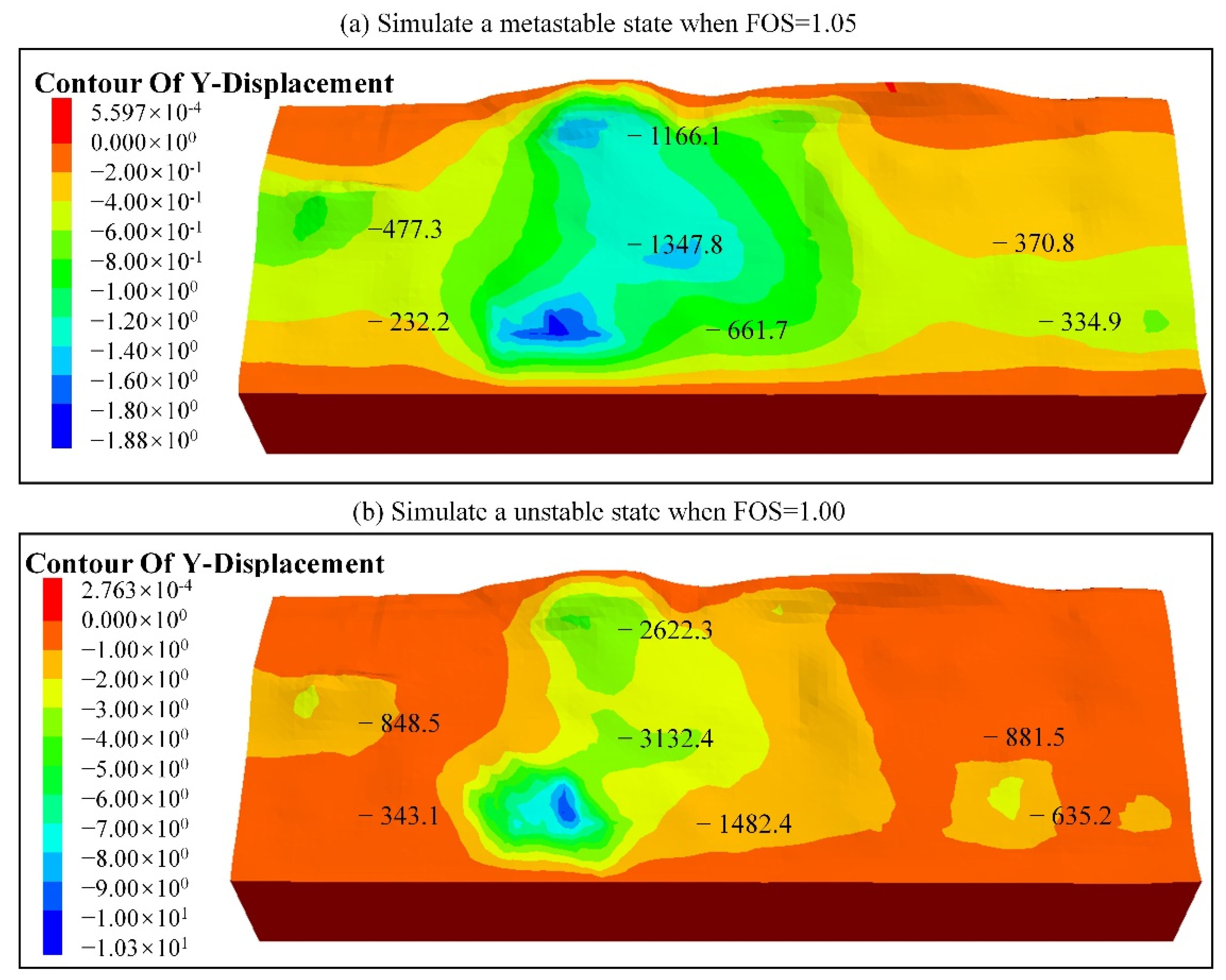
Step 4: Determine the potential failure conditions of the landslide, such as the dynamic excavation, groundwater level changes, etc. Taking the changes in the groundwater level as an example, the seepage module is invoked in the numerical simulation software to simulate and calculate the displacement calculation results under the limit equilibrium state of the landslide by continuously adjusting the water level conditions, and the corresponding warning criteria (e.g., water level and relative displacement thresholds) can be obtained.

3. Results and Discussion

To verify the validity of the proposed method, experiments were designed in the following three parts. In the first part, the deformation mechanism was analyzed based on the GNSS and rainfall data from the monitoring system. In the second part, an orthogonal test scheme was used to generate the training samples, and the validity of the DBA-LSTM algorithm was verified by comparing it to DBA-BPNN. In the third part, based on the measured data, the DBA-LSTM was used to invert the shear strength parameters of this landslide, the equivalent mechanical parameters were substituted into the numerical model, and the corresponding displacement warning thresholds were then calculated by simulating the failure conditions.

3.1. Deformation Mechanism Analysis

From April 2019 to the end of 2019, the system recorded the development of Shangtan landslide deformation process. Figure 7 shows the landslide’s cumulative deformation time series curves and monthly rainfall–time curves (as space is limited, the analysis is conducted for the Y-directional displacement, which has the largest deformation). Significant displacements from the GD03 and GD04 monitoring stations were observed, and the deformation of the Shangtan landslide can be roughly divided into three stages. Slow deformation stage: The accumulated landslide deformation increased slowly in April and May, and the accumulated deformation of the seven GNSS monitoring stations was about 10–20 mm. Evenly accelerated deformation stage: The results from most of the GNSS monitoring stations showed that the landslide deformation displayed an increasing trend in June, and the deformation rate remained stable, with a maximum average rate of 19.2 mm/d and a minimum average rate of 4.8 mm/d. Variable acceleration deformation stage: The GNSS monitoring results show that the landslide entered a stage of accelerated deformation in early July, and the accumulated deformation increased sharply, with the maximum deformation rate of the GD03 and GD04 monitoring stations reaching 119.6 mm/d (15.3 mm/h) and 148.4 mm/d (17.9 mm/h); the accumulated deformation was more than 1 m by the end of September. It is worth stating that the accumulated displacement of GD08 did not exceed 10 mm, indicating that the road foundation is mostly stable and it is an effective relative stability reference station.

By counting the rainfall data, the cumulative rainfall in 2019 was 2806.6 mm, and the cumulative rainfall from July to October was 2400.0 mm, accounting for 86%, with the concentrated rainfall showing obvious time–domain distribution characteristics. According to the relationship between the accumulated landslide deformation and rainfall in Figure 7, it can also be seen that there is an obvious positive correlation between landslide deformation and the concentrated rainfall, and the influence of the concentrated rainfall on the rate of landslide deformation is significant, indicating that rainfall is the main factor inducing the accelerated deformation of the Shangtan landslide.

However, when the displacement data were analyzed using the empirical warning model [43], it was found that the tangent angle calculated at the GD03 and GD04 monitoring stations in July exceeded 85° many times, which indicates that the landslide is in the pro-slide stage.

3.2. Establishment of DBA-LSTM Model

According to the algorithm flow shown in Figure 6, we located the nodes in the grid model based on the coordinates of monitoring stations, with GD01–GD07 corresponding to id = 534, 598, 4334, 2810, 2742, 5336 and 6258, respectively. Then, to determine the inversion parameters, it was already known from previous analyses that rainfall is the main factor influencing landslide deformation, resulting in precipitation seepage through the surface into the landslide, which increases the water content of the sub-clay layer mud and reduces the slip resistance, leading to accelerated landslide creep deformation. Therefore, we took the shear strength parameter of the sub-clay layer as the inversion target parameter. Meanwhile, the infiltration of rainfall would increase the groundwater pressure, and these elevated pressures would, in turn, trigger slope motion, necessitating a fluid–structure interaction analysis for this landslide. The next step was the generation of the training samples and the training of the network model.

3.2.1. Training Samples

The orthogonal test is an effective way to construct DBA-ML samples. It starts with the determination of the test factors and their levels as well as the selection of a reasonable orthogonal table for the table header design based on the factors and levels. Considering that the number of target parameters is six and the interaction between the internal friction angle and cohesion is not considered, we planned to choose an orthogonal table with eight factors and eight levels. According to the field investigation report and some bibliographic data [28,44], we determined the range of values of the target parameters, and the values of other physical and mechanical parameters are listed in

Table 2. Physical and mechanical parameters and target parameters of the landslide.

Group	$\mathit{\rho }/\left(\mathit{t}·{\mathit{m}}^{-3}\right)$	$\mathit{K}/\left(\mathit{M}\mathit{p}\right)$	$\mathit{G}/\left(\mathit{M}\mathit{p}\right)$	$\mathit{c}/\left(\mathit{k}\mathit{p}\right)$	$\mathit{\phi }/\left(°\right)$	$\mathit{M}/\left(\mathit{M}\mathit{p}\right)$	$\mathit{n}/\left(\mathit{\%}\right)$
Sub clay1–3	2200	20–40	13–22	10–14.5	10–16	400	50
Gravel soil	2200	60	36	16	18	1000	50
Bedrock	2900	1300	800	400,000	48	-	-

Note: M is the Biot modulus, and n is the porosity; the other parameters involved in the fluid calculation are Brio coefficient = 1, soil permeability coefficient = ${10}^{-13}$, and water density = 1000 $\mathrm{kg}/{\mathrm{m}}^3$.

, where the levels of the target parameters are determined according to the equal interval principle.

According to the orthogonal table $L_{49}\left(7^8\right)$, a total of 49 FLAC3D forward calculations needed to be arranged, and the Y-directional displacement and vertical displacement of the nodes GD01–GD07 were used as test indicators for the result output (the X-directional displacement was basically neglected, so it is not involved in the analysis, and only the Y-directional and Z-directional displacements were output), and we obtained 49 sets of samples (

Table 3. Training samples.

Num.	Output Layer						Input Layer
	${\mathit{c}}_1$	${\mathit{c}}_2$	${\mathit{c}}_3$	${\mathit{\phi }}_1$	${\mathit{\phi }}_2$	${\mathit{\phi }}_3$	Y	Z
1	10	10	10	10	10	10	−95.4	−57.8
2	10	11	10.75	11	10.75	11	−84.2	−51.8
3	10	12	11.5	12	11.5	12	−76.9	−47.9
4	10	13	12.25	13	12.25	13	−72.5	−45.8
5	10	14	13	14	13	14	−69.6	−44.5
6	10	15	13.75	15	13.75	15	−67.3	−43.4
7	10	16	14.5	16	14.5	16	−65.4	−42.4
8	10.75	10	10.75	12	12.25	14	−94.7	−57.4
9	10.75	11	11.5	13	13	15	−85.2	−52.3
10	10.75	12	12.25	14	13.75	16	−69.7	−42.7
$⋮$
45	14.5	12	10.75	10	14.5	15	−74.9	−49.4
46	14.5	13	11.5	11	10	16	−71.3	−47.6
47	14.5	14	12.25	12	10.75	10	−68.7	−46.3
48	14.5	15	13	13	11.5	11	−58.5	−39.3
49	14.5	16	13.75	14	12.25	12	−57.1	−38.3

). Only some of the arrays are shown in the table, and the input layer information is only populated with the displacement data of node GD03, and data for the other six nodes are not shown. Test samples (

Table 4. Test samples.

Num.	Output Layer						Input Layer
	${\mathit{c}}_1$	${\mathit{c}}_2$	${\mathit{c}}_3$	${\mathit{\phi }}_1$	${\mathit{\phi }}_2$	${\mathit{\phi }}_3$	Y	Z
1	10	10	10	10	10	10	−95.4	−57.8
2	10.75	13	13	15	14.5	10	−66.5	−41.5
3	11.5	12	13	16	10.75	13	−72.6	−44.7
4	11.5	16	10.75	13	13.75	10	−63.3	−42.4
5	12.25	15	10.75	14	10	13	−67.6	−45.0
6	13	16	12.25	10	13	11	−68.5	−47.4
7	14.5	13	11.5	11	10	16	−71.3	−47.6

) were also constructed using the orthogonal tests.

3.2.2. Comparison of DBA-LSTM and DBA-BPNN

The 49 sets of sample data in Table 3 were used as the training sets, the displacement data were treated as the input layer, and the target parameters to be inverted were treated as the output layer for training. According to the literature [19] and the method in this paper, two models, DBA-BPNN and DBA-LSTM, were constructed. By learning the training samples, we determined that the network structure of the DBA-BPNN model was 14-1 (100)-6, which denotes the number of input layers, hidden layers (number of neurons), and output layers, respectively, and the Levenberg–Marquardt algorithm was used as the training algorithm. It should be noted that the number of neurons in the hidden layer calculated by the empirical formula in the literature [19] does not achieve high prediction accuracy, and it was found that: the accuracy is optimal when the number of neurons in the hidden layer is 100; there are two hidden layers in the DBA-LSTM model; the number of neurons in each layer was set to 128 and 64; the tanh function was selected as the activation function; and the number of iterations was set as 10,000 times. The accuracy of DBA-BPNN and DBA-LSTM, respectively, was evaluated using the data in Table 4 as the test sets; Figure 8 shows the fit relationship between the predicted and theoretical values of the two algorithms and the goodness of fit. The six subplots on the left are the results between the predicted values of the DBA-BPNN algorithm and the theoretical values of the samples, corresponding to Figure 9a; the six subplots on the right are the results of the DBA-LSTM algorithm, corresponding to Figure 9b.

Comparing the results of DBA-BPNN and DBA-LSTM, it can be found that both algorithms are in good agreement with the predicted and theoretical values, which indicates that the DBA-ML algorithm can effectively invert the equivalent physical and mechanical parameters of the landslide. However, from Figure 8, it is clear that the fitting effect of DBA-LSTM is significantly better than DBA-BPNN, and by counting the MAPE (average absolute percentage error) of the two algorithms, the accuracy of the DBA-LSTM algorithm (0.62%) is improved by 62.0% compared to the DBA-BPNN algorithm (1.63%).

Among DBA-ML algorithms, the BPNN model was the earliest-applied and is the most frequently employed network model, and the experimental results in this paper show that the accuracy of DBA-LSTM is substantially improved compared to that of DBA-BPNN, but it does not deny the feasibility of DBA-BPNN. In order to further verify the accuracy of the two algorithms in this test, the inversion results of the two algorithms were entered into the numerical model to carry out forward calculation of the landslide displacement, and the actual input displacement data were compared to the actual input displacement data to calculate the differences in the absolute error. The results are shown in Figure 9, where the vertical coordinates correspond to seven groups of test samples.

From the calculation results, it can be seen that for the DBA-BPNN algorithm, the maximum errors of the calculated displacements for this scheme in the Y-direction and Z-direction are 4 mm and 2 mm, respectively, but from Figure 9a,c, it can be seen that DBA-BPNN only demonstrates large deviations at GD03 and GD04. Considering that the relative displacement of these two stations is much larger than others, by calculating the relative errors, it was found that the relative error is less than 5% for all of the stations in the seven groups of samples. Therefore, the DBA-BPNN algorithm is feasible for landslide inversion. The computational accuracy of the DBA-LSTM algorithm in both the Y- and Z-directions is less than 1 mm, which indicates that the landslide parameters in the inversion of the DBA-LSTM algorithm are more accurate.

In short, machine learning for displacement back-analysis can effectively invert the equivalent physical and mechanical parameters with higher accuracy, but the deep learning algorithm has better prediction performance in terms of landslide inversion.

3.3. Determination of the Warning Thresholds

3.3.1. Parameters Inversion Using DBA-LSTM

The period from April to June 2019 was used as the input parameter for the DBA-LSTM model, the shear strength parameters in the numerical model were modified, and the RMSEs in the Y- and Z-directions were calculated to be 3.9 mm and 1.8 mm, with a maximum deviation of 6.1 mm at the point, indicating that the numerical simulation results are basically consistent with the field monitoring results and that the analytical model can be further used for stability analysis. Figure 10 shows the displacement in the Y-direction calculated based on the inversion results, where the data in the figure represent the calculated displacement values of each monitoring station. The displacement nephograms in the X- and Z-directions are not shown, due to space limitations.

3.3.2. Numerical Analysis

Based on the modified model, the stability of the current state of the landslide was analyzed according to the strength reduction method, and the FOS was calculated to be 1.38. According to the Technical Code for Building Slope Engineering (GB50330-2013) published by the Chinese Ministry of Housing and Urban–Rural Development, it can be determined that Shangtan landslide was in a stable state at the end of June.

A follow-up was carried out to determine the warning criterion for different landslide stages according to the evolutionary conditions. Simulating the deformation of this landslide, apart from considering the changes in the stress field under the action of gravity, the changes in the pore pressure field generated by groundwater changes and seepage should also be considered. First, two combinations of shear strength parameters with safety factors of 1.05 and 1.10 were obtained according to the discount factor, and the ultimate groundwater level was set to simulate two cases: the metastable state and unstable state, and the calculation results are shown in Figure 11. The upper part of the figure shows the displacement calculation results when the simulated safety factor was 1.05 (i.e., sub-stable state), and the bottom part of the figure shows the displacement calculation results of the unstable state.

According to the calculation results of the two evolutionary states, two sets of displacement warning criteria can be set (

Table 5. Two sets of displacement warning thresholds (unit/mm).

State	GD01	GD02	GD03	GD04	GD05	GD06	GD07
metastable	−477.3	−232.2	−1166.1	−1347.8	−661.7	−370.8	−334.9
unstable	−848.5	−343.1	−2622.3	−3132.4	−1482.4	−881.5	−635.2

). When the relative displacement monitoring results reach the first set of thresholds, it means that the landslide is in a metastable state and should take corresponding management measures, and when the displacement reaches the second set of thresholds, it means that the landslide is about to become unstable and emergency warning measures should be taken.

3.3.3. Verification of the Warning Thresholds

The tangent angles obtained from GD03 and GD04 in July exceeded 85° several times, implying that the empirical warning model predicted that the landslide would show signs of damage in July. However, according to the GNSS displacement monitoring results from July to September (

Table 6. July–September GNSS displacement monitoring sequence (unit/mm).

Time	GD01	GD02	GD03	GD04	GD05	GD06	GD07
7/15	−75.2	−32.5	−531.0	−838.3	−34.1	−25.0	−23.0
7/31	−75.0	−31.9	−844.3	−1188.3	−34.2	−23.4	−22.6
8/15	−74.4	−27.8	−839.7	−1187.7	−36.4	−21.6	−21.2
8/31	−88.9	−39.0	−1128.7	−1430.6	−43.1	−28.3	−30.0
9/15	−112.0	−49.6	−1434.4	−1689.8	−46.6	−29.9	−37.7
9/30	−109.5	−44.7	−1430.9	−1684.7	−44.5	−30.6	−29.8

), in which the same GD03 and GD04 monitoring stations were used as the target of analysis, and assuming that landslide deformation usually develops until mid-September, the measured results of the model are still some distance away from the second set of unstable warning criteria, indicating that the method in this paper indicates that the landslide will not be destabilized and will be in a metastable state. Thus, the method of this paper obtained results that were different from the warning results of the empirical model.

According to the accumulated deformation in 2019 (Figure 7) and the information in Table 6, it can be seen that the accelerated deformation trend of the Shangtan landslide stabilized in mid-September. Meanwhile, according to the site inspection results after the accelerated landslide deformation (Figure 12), we found that some new cracks appeared at the site but that no phenomena such as slippage or collapse were observed, which verifies the feasibility of the warning results of the proposed method and allows incorrect warnings to be avoided.

4. Conclusions

Landslide deformation and damage occur under the joint action of various influencing factors such as geological conditions, rainfall, and groundwater. This study takes the Shangtan landslide as the research object and determines the interaction mechanism between the geological structure, mechanical mechanism, and landslide deformation by constructing a modifiable numerical model, and the damage mechanism of this landslide was analyzed by numerical simulation. Moreover, a novel approach using deep learning algorithms for displacement back-analysis was proposed for the first time.

Based on the GNSS and rainfall data, we found the Shangtan landslide showed slow deformation, uniformly accelerated deformation, and variable accelerated deformation, with the largest cumulative displacement change in being observed in the north–south direction and the maximum deformation rate reaching 148.4 mm/d. Furthermore, the concentrated rainfall in the rainy season led to the softening of the sub-clay layer and a reduction in the slip resistance strength, which was the main reason for the variable accelerated deformation of the landslide. Particularly, to determine the shear strength parameters of the sub-clay layer, two DBA-ML models were constructed, and both algorithms showed satisfactory performance in terms of prediction accuracy, demonstrating relative errors of less than 5%. The DBA-LSTM algorithm improved the computational accuracy by 62.0% compared to DBA-BPNN, implying that the deep learning algorithm has better landslide displacement back-analysis performance. However, the prediction ability of both algorithms was dependent on the accuracy of the model parameter settings. Therefore, the application of the Auto-ML technique for displacement back-analysis to enable the model to learn the appropriate parameters automatically is also one of the important works in the subsequent research. Furthermore, to accurately assess the degree of landslide stability, a novel landslide warning method based on DBA-LSTM and the numerical analysis algorithms was proposed. Two sets of displacement warning criteria corresponding to two levels of the metastable state and unstable state were determined by numerical simulations. The validation results show that the criteria in this paper are more reasonable than those of the empirical warning model and have a certain reference value for landslide hazard warnings.

References

1. Niu, X.; Ma, J.; Wang, Y.; Zhang, J.; Chen, H.; Tang, H. A Novel Decomposition-Ensemble Learning Model Based on Ensemble Empirical Mode Decomposition and Recurrent Neural Network for Landslide Displacement Prediction. Appl. Sci. 2021, 11, 4684. [Google Scholar] [CrossRef]
2. Yin, Y.; Zheng, W.; Liu, Y.; Zhang, J.; Li, X. Integration of GPS with InSAR to monitoring of the Jiaju landslide in Sichuan, China. Landslides 2010, 7, 359–365. [Google Scholar] [CrossRef]
3. Zhu, W.; Zhang, Q.; Ding, X.L.; Zhao, C.Y.; Yang, C.S.; Qu, F.F.; Qu, W. Landslide monitoring by combining of CR-InSAR and GPS techniques. Adv. Space Res. 2014, 53, 430–439. [Google Scholar] [CrossRef]
4. Fan, X.M.; Xu, Q.; Scaringi, G.; Dai, L.X.; Li, W.L.; Dong, X.J.; Zhu, X.; Pei, X.J.; Dai, K.R.; Havenith, H.B. Failure mechanism and kinematics of the deadly June 24th 2017 Xinmo landslide, Maoxian, Sichuan, China. Landslides 2017, 14, 2129–2146. [Google Scholar] [CrossRef]
5. Zhu, Y.; Qiu, H.; Yang, D.; Liu, Z.; Ma, S.; Pei, Y.; He, J.; Du, C.; Sun, H. Pre- and post-failure spatiotemporal evolution of loess landslides: A case study of the Jiangou landslide in Ledu, China. Landslides 2021, 18, 3475–3484. [Google Scholar] [CrossRef]
6. Qiao, N.; Duan, Y.-L.; Shi, X.-M.; Wei, X.-F.; Feng, J.-M. Study on the Early Warning Methods of Dynamic Landslides of Large Abandoned Rockfill Slopes. Appl. Sci. 2020, 10, 6097. [Google Scholar] [CrossRef]
7. Smethurst, J.A.; Smith, A.; Uhlemann, S.; Wooff, C.; Chambers, J.; Hughes, P.; Lenart, S.; Saroglou, H.; Springman, S.M.; Lofroth, H.; et al. Current and future role of instrumentation and monitoring in the performance of transport infrastructure slopes. Q. J. Eng. Geol. Hydrogeol. 2017, 50, 271–286. [Google Scholar] [CrossRef] [Green Version]
8. Xu, L.; Cheng, G.; Zhu, H.H. Research Review of Landslide Monitoring Methods Based on Integration of Space-Air-Ground-Interior. Laser Optoelectron. Prog. 2021, 58, 0900006. [Google Scholar] [CrossRef]
9. Uhlemann, S.; Smith, A.; Chambers, J.; Dixon, N.; Dijkstra, T.; Haslam, E.; Meldrum, P.; Merritt, A.; Gunn, D.; Mackay, J. Assessment of ground-based monitoring techniques applied to landslide investigations. Geomorphology 2016, 253, 438–451. [Google Scholar] [CrossRef] [Green Version]
10. Abraham, M.T.; Satyam, N.; Pradhan, B.; Segoni, S.; Alamri, A. Developing a prototype landslide early warning system for Darjeeling Himalayas using SIGMA model and real-time field monitoring. Geosci. J. 2022, 26, 289–301. [Google Scholar] [CrossRef]
11. Huang, J.; van Asch, T.W.J.; Wang, C.M.; Li, Q. Study on the combined threshold for gully-type debris flow early warning. Nat. Hazards Earth Syst. Sci. 2019, 19, 41–51. [Google Scholar] [CrossRef] [Green Version]
12. Liang, W.L. Dynamics of pore water pressure at the soil-bedrock interface recorded during a rainfall-induced shallow landslide in a steep natural forested headwater catchment, Taiwan. J. Hydrol. 2020, 587, 125003. [Google Scholar] [CrossRef]
13. Wang, H.L.; Jiang, Z.H.; Xu, W.Y.; Wang, R.B.; Xie, W.C. Physical model test on deformation and failure mechanism of deposit landslide under gradient rainfall. Bull. Eng. Geol. Environ. 2022, 81, 66. [Google Scholar] [CrossRef]
14. He, M.C.; Tao, Z.G.; Gong, W.L. Geo-disaster prediction with double-block mechanics based on Newton force measurement. Geomech. Geophys. Geo-Energy Geo-Resour. 2017, 3, 107–119. [Google Scholar] [CrossRef]
15. Basharat, M.; Riaz, M.T.; Jan, M.Q.; Xu, C.; Riaz, S. A review of landslides related to the 2005 Kashmir Earthquake: Implication and future challenges. Nat. Hazards 2021, 108, 1–30. [Google Scholar] [CrossRef]
16. He, M.C.; Ren, S.L.; Tao, Z.G. Remote monitoring and forecasting system of Newton force for landslide geological hazards and its engineering application. Chin. J. Rock Mech. Eng. 2021, 40, 2161–2172. [Google Scholar] [CrossRef]
17. Xie, W.L.; Guo, Q.Y.; Wu, J.Y.; Li, P.; Yang, H.; Zhang, M.S. Analysis of loess landslide mechanism and numerical simulation stabilization on the Loess Plateau in Central China. Nat. Hazards 2021, 106, 805–827. [Google Scholar] [CrossRef]
18. Zhang, Y.G.; Zhang, Z.; Xue, S.; Wang, R.J.; Xiao, M. Stability analysis of a typical landslide mass in the Three Gorges Reservoir under varying reservoir water levels. Environ. Earth Sci. 2020, 79, 42. [Google Scholar] [CrossRef]
19. Jiang, J.W.; Ehret, D.; Xiang, W.; Rohn, J.; Huang, L.; Yan, S.J.; Bi, R.N. Numerical simulation of Qiaotou Landslide deformation caused by drawdown of the Three Gorges Reservoir, China. Environ. Earth Sci. 2011, 62, 411–419. [Google Scholar] [CrossRef]
20. Zhang, Y.G.; Zhu, S.Y.; Tan, J.K.; Li, L.D.; Yin, X.J. The influence of water level fluctuation on the stability of landslide in the Three Gorges Reservoir. Arab. J. Geosci. 2020, 13, 845. [Google Scholar] [CrossRef]
21. Ding, M.T.; Cai, C.F.; Qin, H.Z. Accumulation landslide stability analysis based on FLAC numerical simulation. Disaster Adv. 2012, 5, 1783–1790. [Google Scholar]
22. Wang, H.; Tian, G.; Zhao, Y.H.; Xie, Y.Q.; Zhang, Q.; Xu, A.D.; Li, X.F. Dynamic modeling of Meiping landslide process. Nat. Hazards 2019, 96, 879–892. [Google Scholar] [CrossRef]
23. Feng, X.T.; Zhang, Z.Q.; Sheng, Q. Estimating mechanical rock mass parameters relating to the Three Gorges Project permanent shiplock using an intelligent displacement back analysis method. Int. J. Rock Mech. Min. Sci. 2000, 37, 1039–1054. [Google Scholar] [CrossRef]
24. Deng, J.H.; Lee, C.G. Displacement back analysis for a steep slope at the Three Gorges Project site. Int. J. Rock Mech. Min. Sci. 2001, 38, 259–268. [Google Scholar] [CrossRef]
25. Zhang, Y.; Su, G.S.; Liu, B.C.; Li, T.B. A novel displacement back analysis method considering the displacement loss for underground rock mass engineering. Tunn. Undergr. Space Technol. 2020, 95, 103141. [Google Scholar] [CrossRef]
26. Zhuang, D.; Ma, K.; Tang, C.; Liang, Z.; Wang, K.; Wang, Z. Mechanical parameter inversion in tunnel engineering using support vector regression optimized by multi-strategy artificial fish swarm algorithm. Tunn. Undergr. Space Technol. 2019, 83, 425–436. [Google Scholar] [CrossRef]
27. Li, S.J.; Zhao, H.B.; Ru, Z.L.; Sun, Q.C. Probabilistic back analysis based on Bayesian and multi-output support vector machine for a high cut rock slope. Eng. Geol. 2016, 203, 178–190. [Google Scholar] [CrossRef]
28. Xing, H.; Zhang, H.; Liu, L.; Yao, D. Comprehensive monitoring of talus slope deformation and displacement back analysis of mechanical parameters based on back-propagation neural network. Landslides 2021, 18, 1889–1907. [Google Scholar] [CrossRef]
29. Zhang, X.; Zhu, C.; He, M.C.; Dong, M.L.; Zhang, G.C.; Zhang, F.M. Failure Mechanism and Long Short-Term Memory Neural Network Model for Landslide Risk Prediction. Remote Sens. 2022, 14, 166. [Google Scholar] [CrossRef]
30. Ma, H.S.; Wang, H.L.; Wang, R.B.; Meng, Q.X.; Yang, L.L. Automatic back analysis of mechanical parameters using block discrete element method and PSO algorithm. Eur. J. Environ. Civ. Eng. 2020, 1–11. [Google Scholar] [CrossRef]
31. Zhang, Y.; Su, G.S.; Li, Y.; Wei, M.D.; Liu, B.C. Displacement Back-Analysis of Rock Mass Parameters for Underground Caverns Using a Novel Intelligent Optimization Method. Int. J. Geomech. 2020, 20, 04020035. [Google Scholar] [CrossRef]
32. Hinton, G.E.; Salakhutdinov, R.R. Reducing the dimensionality of data with neural networks. Science 2006, 313, 504–507. [Google Scholar] [CrossRef] [Green Version]
33. Liu, Z.Q.; Guo, D.; Lacasse, S.; Li, J.H.; Yang, B.B.; Choi, J.C. Algorithms for intelligent prediction of landslide displacements. J. Zhejiang Univ.-Sci. A 2020, 21, 412–429. [Google Scholar] [CrossRef]
34. Bui, D.; Tsangaratos, P.; Nguyen, V.T.; Liem, N.V.; Trinh, P.T. Comparing the prediction performance of a Deep Learning Neural Network model with conventional machine learning models in landslide susceptibility assessment. Catena 2020, 188, 104426. [Google Scholar] [CrossRef]
35. Mandal, K.; Saha, S.; Mandal, S. Applying deep learning and benchmark machine learning algorithms for landslide susceptibility modelling in Rorachu river basin of Sikkim Himalaya, India. Geosci. Front. 2021, 12, 101203. [Google Scholar] [CrossRef]
36. Weissmann, G.S.; Fogg, G.E. Multi-scale alluvial fan heterogeneity modeled with transition probability geostatistics in a sequence stratigraphic framework. J. Hydrol. 1999, 226, 48–65. [Google Scholar] [CrossRef]
37. Makaske, B. Anastomosing rivers: A review of their classification, origin and sedimentary products. Earth-Sci. Rev. 2001, 53, 149–196. [Google Scholar] [CrossRef]
38. Bai, D.; Tang, J.; Lu, G.; Zhu, Z.; Liu, T.; Fang, J. The design and application of landslide monitoring and early warning system based on microservice architecture. Geomat. Nat. Hazards Risk 2020, 11, 928–948. [Google Scholar] [CrossRef]
39. Zheng, D.J.; Cheng, L.; Bao, T.F.; Lv, B.B. Integrated parameter inversion analysis method of a CFRD based on multi-output support vector machines and the clonal selection algorithm. Comput. Geotech. 2013, 47, 68–77. [Google Scholar] [CrossRef]
40. Wang, J.; Jiang, W.; Li, Z.; Lu, Y. A New Multi-Scale Sliding Window LSTM Framework (MSSW-LSTM): A Case Study for GNSS Time-Series Prediction. Remote Sens. 2021, 13, 3328. [Google Scholar] [CrossRef]
41. Chen, L.; Jin, X. Study on the applicability of three criteria for slope instability using finite element strength reduction method. China Civ. Eng. J. 2012, 45, 136–146. [Google Scholar] [CrossRef]
42. Wang, J.J.; Liang, Y.; Zhang, H.P.; Wu, Y.; Lin, X. A loess landslide induced by excavation and rainfall. Landslides 2014, 11, 141–152. [Google Scholar] [CrossRef]
43. Xu, Q.; Zeng, Y.; Qian, J.; Wang, C.; He, C. Study on a improved tangential angle and the corresponding landslide prewarning criteria. Geol. Bull. China 2009, 28, 501–505. [Google Scholar]
44. Heidemann, M.; Bressani, L.A.; Flores, J.A. Hydrothermal clays and their influence on slope stability in residual soils of Southern Brazil. Bull. Eng. Geol. Environ. 2021, 80, 795–811. [Google Scholar] [CrossRef]
Figure 1. Location of the Shangtan landslide.
Applsci 12 06690 g001
Figure 2. The 3D mesh model of the Shangtan landslide.
Applsci 12 06690 g002
Figure 3. Gutter extrusion deformation (left); retaining wall cracking (right).
Applsci 12 06690 g003
Figure 4. Location of landslide monitoring stations.
Applsci 12 06690 g004
Figure 5. (a) LSTM network model structure; (b) LTSM cell structure.
Applsci 12 06690 g005
Figure 6. Threshold calculation process.
Applsci 12 06690 g006
Figure 7. Monitoring data.
Applsci 12 06690 g007
Figure 8. Fitting relationship and goodness of fit R 2 .
Applsci 12 06690 g008
Figure 9. Residual plots.
Applsci 12 06690 g009
Figure 10. Simulated displacement nephogram based on the inversion results.
Applsci 12 06690 g010
Figure 11. Displacement simulation results for a given evolutionary condition.
Applsci 12 06690 g011
Figure 12. Field inspection photos. (a) Around the station of GD01. (b) Station of GD03. (c) Station of GD03. (d) Around the station of GD04.
Applsci 12 06690 g012