A Clustering Algorithm for Evolving Data Streams Using Temporal Spatial Hyper Cube

Abstract

As applications generate massive amounts of data streams, the requirement for ways to analyze and cluster this data has become a critical field of research for knowledge discovery. Data stream clustering’s primary objective and goal are to acquire insights into incoming data. Recognizing all possible patterns in data streams that enter at variable rates and structures and evolve over time is critical for acquiring insights. Analyzing the data stream has been one of the vital research areas due to the inevitable evolving aspect of the data stream and its vast application domains. Existing algorithms for handling data stream clustering consider adding various data summarization structures starting from grid projection and ending with buffers of Core-Micro and Macro clusters. However, it is found that the static assumption of the data summarization impacts the quality of clustering. To fill this gap, an online clustering algorithm for handling evolving data streams using a tempo-spatial hyper cube called BOCEDS TSHC has been developed in this research. The role of the tempo-spatial hyper cube (TSHC) is to add more dimensions to the data summarization for more degree of freedom. TSHC when added to Buffer-based Online Clustering for Evolving Data Stream (BOCEDS) results in a superior evolving data stream clustering algorithm. Evaluation based on both the real world and synthetic datasets has proven the superiority of the developed BOCEDS TSHC clustering algorithm over the baseline algorithms with respect to most of the clustering metrics.

1. Introduction

Data streams are a continuous, infinite series of data records followed and arranged by embedded or precise timestamps [1]. With sensors becoming prevalent in humans’ daily lives, it’s clear that the availability of data streams is exponentially increasing [2]. Mainly driven by the expansion of the Internet of Things (IoT) and the connected real-time data sources, many application domains, generate an infinitely vast amount of critical data streams that evolve [3]. For an instance, urban pop-up housing environments and their potential as local innovation systems are a source of a massive data stream generator [4]. Analyzing such data stream efficiently offers useful insights for many application domains. Yet, as applications generate massive amounts of data, the requirement for methods to analyze and cluster data streams has become a critical field of research for knowledge discovery [5,6]. Data stream clustering’s primary objective and goal are to acquire insights into incoming data. Recognizing all possible patterns in the data that enters at varying speeds and structures and evolves over time is critical for this analysis process [7].

Clustering data streams is one of the vital tasks in data stream analysis to identify the abstract of hidden themes coherently that characterize the stream. It is defined as the technique for partitioning the data in the data stream into clusters where similar data are placed in the same cluster, and dissimilar data are placed in another cluster [8]. It is an unsupervised learning method that has become a useful, ubiquitous, and essential tool for data stream analysis in machine learning, data mining, bioinformatics, image processing, and other fields. Yet, data streams impose additional challenges on clustering, such as clustering in limited memory, limited time, high-dimensionality, analyzing the data only once as it arrives and handling data in evolving manner to capture the underlying changes in clusters [9]. Unlike batch processing, there’s no complete dataset available [10]. Data stream clustering algorithms analyze each data record as it arrives in sequential order and any processing or learning requires to be performed online, where stored data are not available for further analysis [11].

Clustering data stream require algorithms to have the capability of evolving their structure and paraments with respect to time and as new data streams arrive. Unlike static data, detection algorithms struggle for adapting the dynamic environments such as the ever-evolving IoT domain [12]. Furthermore, the data streams that regularly originated from non-stationary environments with no advanced information regarding the data distribution, could affect the choice of a suitable set of algorithm parameters for detecting anomalies. Moreover, in most real-life cases, a massive amount of data streams coming from the enormous number of IoT sensors is almost impossible to label coming from the enormous number of IoT sensors, Therefore, working in an unsupervised fashion is always a necessity [13].

The literature contains numerous algorithms that aim at solving the issues of data stream clustering. Various challenging elements were considered for solving the problem. In the work of CEDAS [14] and BOCEDS [15], the author has enabled an arbitrary shape clustering algorithm to perform the clustering with an evolving cluster. The cluster might take any possible shape and its shape might change with respect to time. However, a significant issue is observed in these algorithms. The lack of quantization stage of the raw data before dealing with it in the creation of the core mini clusters. Other algorithms have adopted the grid concept for this quantization such as MuDi-Stream [16]. However, they used a static grid in both time and spatial attributes.

The goal of this research is to address the problem of evolving data stream clustering with arbitrary positioning and shaping of clusters. This could be achieved by designing and developing an online clustering algorithm for handling evolving data streams using the tempo-spatial hyper cube called BOCEDS TSHC. The contributions of this research are as follows:

i.

The proposed BOCEDS TSHC uses a tempo-spatial hyper cube to add more dimensions to the data summarization for more degree of freedom.

The hyper-cube is a quantization level that will map various values to one value in each coordinate to reduce the resolution of data storing and eliminate the effect of slight changes that do not influence the meaning of the data (type of filtering). The hyper-cube features heterogeneity to handle heterogeneous data and dynamicity to handle the evolving data according to the values of its features or coordinates.

ii.

The TSHC algorithm is built using the recursive and dynamic update for adaptive quantization of arrived data when they are projected to the clustering space.

iii.

The developed TSHC algorithm is an add-on to a single-phase clustering algorithm that assists in generating clusters from evolving data streams in a fully online manner. It can work independently or jointly with an existing clustering algorithm such as BOCEDS.

The remaining paper is organized as follows. Section 2 presents a literature review of the latest clustering algorithms. Section 3 discusses the research methodology used in this research, which includes the description of the developed algorithm. Section 4 illustrates the results and discussion of the research followed by Section 5, which presents the findings and summary. Finally, Section 6, concludes the paper.

2. Literature Review

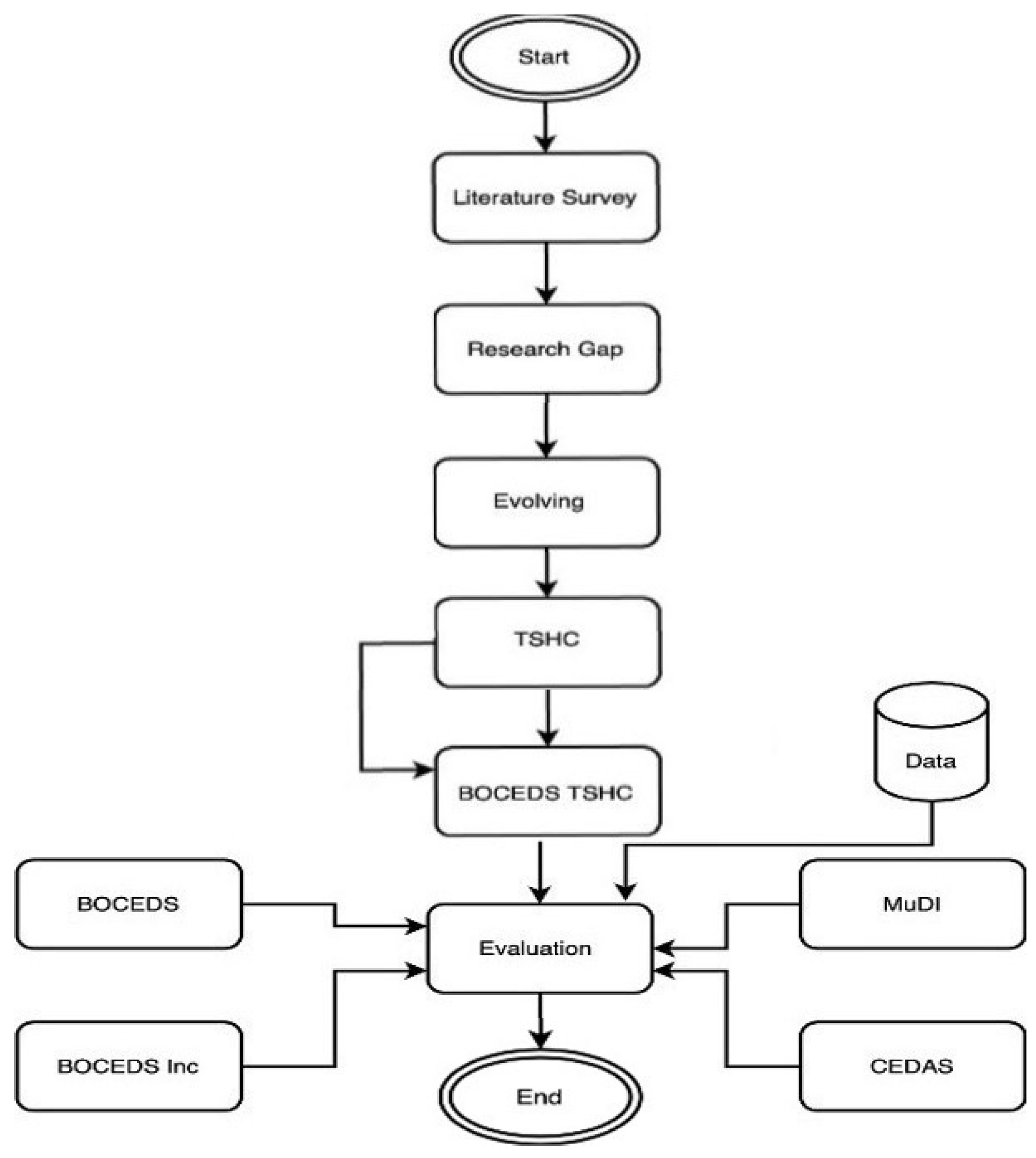
Among the first online clustering algorithms, an algorithm called clustering online data streams into arbitrary shapes (CODAS) [17], was introduced to enable the generation of arbitrary shaped clusters for real-time data streams. CODAS is a data-driven algorithm that constructs micro-clusters to summarize data points and then scales to multi-dimensional data streams. Yet, in CODAS, the generated clusters are not capable of evolving.

After that, CODAS was enhanced and CEDAS was proposed by [14], CEDAS introduces a simple linear aging mechanism to deal with the evolving features of data streams. This is the first technique to perform live clustering fully on evolving data streams. CEDAS is divided into two stages. The first phase involves the creation of micro-clusters or the insertion of data into existing micro-clusters, followed by information correction. The second phase involves intersecting micro-clusters and grouping them into kernel and shell areas. Every macro-cluster in this method contains a graph illustrating intersecting micro-clusters for every micro-cluster. The adjacency relations are stored as a property of the micro-cluster. CEDAS quickly produces high-quality clustering results and is capable of coping with the dynamic features of a data stream and outliers. CEDAS, like other density-based clustering techniques, requires a significant amount of processing time.

Concurrently, a novel framework for clustering the evolving data stream called Cauchy was proposed [18]. It is an online technique that can adjust to the classifier in real-time. Additionally, the authors propose a strategy for developing a cyber-attack detection technique. The technique was evaluated using a 1999 KDD intrusion detection database to tackle the costly and time-consuming issues associated with traditional offline methods. The findings indicate that the cost of labeling learning data was reduced. Due to the online nature of this approach, adding definitions for new threats is considerably easier and simpler than with batch learning methods. Nevertheless, as with other density-based clustering methods, the Cauchy technique has a significant disadvantage: it lacks a mechanism for merging clusters, which would reduce the number of clusters formed, and it is inefficient for high-dimensional data.

In the same year, an algorithm called xStream was introduced to address the problem of features evolving in data streams [10]. This work addresses a previously unstudied problem by proposing xStream, which is a density-based ensemble anomaly detector with the following three characteristics: (1) it is a constant-space and constant-time (per incoming update) algorithm, (2) it detects anomalies at multiple scales or granularities, and (3) it can handle (3i) high-dimensionality via distance-preserving projections and (3ii) non-stationarity via O (1)-time model updates as the stream progresses. However, no attempt was made to address the issue of cluster evolving, which affects the overall outlier detection.

Furthermore, in [19], the authors presented a technique called Online Clustering for Evolving Data Streams with Anomaly Detection (OnCAD). The suggested technique considers both the temporal and spatial proximity of observations to detect abnormalities in real-time. It detects cluster evolution in noisy streams, incrementally updates the model, and calculates the minimal window length over the evolving data stream without sacrificing speed. Nonetheless, the technique is incapable of dealing with high-dimensional data, as clusters of data typically occur in a subspace of the original input space.

Another enhanced version of CODAS is named i-CODAS. It operates based on the concept of maintaining the local radius for each micro-cluster independently [20]. CODAS, like other density-based clustering methods, maintains a global and constant radius for each micro-cluster. However, setting the appropriate micro-cluster radius is extremely difficult in practice, and a global radius might not even be optimal for each micro-cluster. A poor choice of radius significantly degrades the clustering quality. To address this issue, i-CODAS updates the radius in real-time to its local optimal value whenever a new data sample is added to the cluster. Metadata, referred to as micro-clusters, is used to summarize the data samples. The micro-clusters are visualized in a clustering graph based on their connectedness. Finally, the clustering graph is utilized to build clusters of any shape. Nonetheless, one of the algorithm’s primary drawbacks is its high memory requirement.

As an improvement of CEDAS, a fully online density-based clustering algorithm called buffer-based online clustering for evolving data stream BOCEDS was introduced by [15]. This technique changes the micro-cluster radius iteratively until it reaches its local optimal value, which was one of the restrictions described on CEDAS. BOCEDS additionally provides a buffer for storing unnecessary micro-clusters and a fully online pruning mechanism for removing the buffer’s momentarily irrelevant micro-clusters. Experimental results prove BOCEDS’s superiority over the other clustering algorithms. Yet, the study fails to decrease the memory consumption without impairing other clustering performance criteria. Furthermore, the study also failed to identify false merging for overlapped clusters.

Similarly, an online incremental clustering framework named OICF-Stream was presented for data stream analytics [21]. It is a strategy that employs an incremental clustering technique to operate within real-time limitations, in real-time, while maintaining accuracy. The experimental results reveal that the proposed strategy is superior in terms of accuracy and has a significant improvement in execution time. However, the created algorithm is incapable of handling multidimensional data streams and so consumes a great deal of processing power.

Another online dynamic clustering method for tracking evolving environments called DyClee was proposed by [22]. It is a unified approach to monitoring developing environments that use a two-stage clustering technique based on distance and density. In this approach, data samples are incrementally fed online into the distance-based clustering stage, where they are grouped to generate μ-clusters. To generate the final clusters, the density-based algorithm analyses the micro-clusters. Additionally, the approach is capable of recognizing clusters with a high degree of overlap even in multi-density distributions without making any assumptions regarding cluster convexity. The experimental results demonstrate that the suggested approach responds quickly to data streams and has a high rate of outlier rejection. However, the proposed technique does not account for drift data stream clustering.

Recently, a new online method called CEDGM was proposed by [23], which is a technique for clustering data streams based on a density grid. The density grid-based technique’s key goals are to minimize distant function calls as well as to increase cluster quality. The technique is fully online and is divided into two distinct phases. The first phase is responsible for generating the Core Micro-Clusters (CMCs), while the second phase merges the CMCs to form macro clusters. The grid-based technique was used as an outlier buffer to manage data with varying densities and noise. The developed technique was shown to be an effective solution for minimizing distance function calls and enhancing cluster quality. Nonetheless, one of the CEDGM algorithm’s shortcomings when dealing with high-dimensional data is the grid’s ineffectiveness at lowering memory usage, particularly for high-dimensional data that are sparse in nature.

A recent fully online clustering algorithm for evolving data-stream based on data point density called OCED was proposed by [24]. The technique clusters the data points into a sphere-shaped data structure known as a micro-cluster. The initial radius of the micro-cluster is learned and adjusted according to the average data point density. A cluster graph is constructed in real-time utilizing micro-clusters to generate the arbitrarily shaped cluster. To deal with the developing property, micro-clusters that are irrelevant to recent data-stream content are recognized and eliminated. However, the approach is limited to numerical attributes, rendering it incapable of handling data streams with mixed attribute types.

CeAC is another recently proposed completely online clustering technique based on grid density [25]. It is a cost-effective and adaptive clustering technique that can increase computational efficiency while maintaining the clustering result’s accuracy. CeAC can generate clusters of any shape and efficiently cope with outliers in parallel. Additionally, it has an adaptive calculating approach that speeds up clustering operations by shedding workload based on the characteristics of the incoming data. The suggested method is accurate and efficient in real-time data stream clustering, as demonstrated by experimental findings. However, the suggested technique does not address the issue of clusters merging incorrectly, which is a regular occurrence when dealing with developing data streams.

To summarize, existing literature contains numerous approaches that aim at solving the problem of clustering evolving data streams. Various challenging elements were considered for solving the problem. In the work of CEDAS [5] and BOCEDS [15], the authors have enabled arbitrary shape clustering algorithm to perform the clustering with evolving cluster (the cluster might take any possible shape and its shape might change with respect to time). However, significant issues are observed in these algorithms. There is a lack of quantization stage of the raw data before dealing with it in the creation of the core mini clusters. Other algorithms have adopted the grid concept for this quantization, such as MuDi-Stream [26]; however, they used the static grid in time and spatial attributes.

3. Methodology

This research aims to design and develop an online clustering algorithm for handling evolving data streams. To achieve this, this paper develops an online clustering algorithm for handling evolving data streams using a tempo-spatial hyper cube. The developed methodology is presented in Figure 1. As it is shown, it starts with the literature survey followed by the research gap. The research gap focuses on the evolving aspect of the data. The handling of evolving will be conducted by designing an online clustering algorithm for handling evolving data streams using tempo-spatial hyper cube. Afterward, the baseline approach that is BOCEDS is implemented. Integrating the research objective with BOCEDS yields an algorithm called: BOCEDS-TSHC. The evaluation of the performance is based on comparing the developed BOCEDS-TSHC algorithm using standard evaluation metrics and benchmarking datasets. The benchmarks algorithms are BOCEDS [15], CEDAS [14] and MuDi-Stream [16]. The datasets used for the evaluation are DNA, Spiral, Landsat, KDD Cup’99, and Traffic Datasets. A visualization of some of the used datasets is presented in Figure 2, which illustrates the evolving behavior of the datasets. The performance of the developed BOCEDS-TSHC algorithm is evaluated using two types of evaluation namely, quality and efficiency evaluation.

3.1. Definitions of Algorithm Parameters

Before executing the developed algorithms, some dependent parameters are set based on expert knowledge in the field, as is the case with other density-based clustering algorithms such as BOCEDS, BOCEDS Inc, CEDAS, and MuDi-Stream. The developed algorithms define the following clustering parameters.

• Inc Step for Quantization: The step that is used for increasing the quantization at any dimension to fulfill the condition given in the inequality of Equation (1).
• Initial quantization level (q₀): The value that is given as the initial quantization level when starting the algorithm.
• Decay: Decay is the number of data points that arrive per unit time from the data stream. It is the data transfer rate. A decay of 50 indicates that 50 data points are extracted consecutively from the data stream on average per unit time (second, minute). It is utilized to keep the energy of micro-clusters up to date. This value is determined based on the application’s expert knowledge.
• Maximum (R_max) and Minimum (R_min): The maximum and minimum radii of micro-clusters are determined using professional knowledge of the application. The maximum radius demonstrates the separation and smoothness of micro-clusters, whilst the minimum radius demonstrates the development of micro-clusters with enough data points.
• CM Threshold: The density threshold that is used to convert the data arrived at a certain grid to a core micro-cluster.
• Cell Threshold: The threshold used to determine when the Tempo Spatial Hyper Cube has converged, and no additional quantization level increments are required in any dimension.
• Outlier Threshold: The density threshold that is used to convert a CM to an outlier for removing it.

3.2. Parameters Setting

The operation of almost all the algorithms depends strongly on the initialization of its parameters. Prior to the execution of the developed algorithm, the selected parameters for the developed algorithm alongside the benchmark algorithms are set based on a tuning technique to accomplish the best possible performance using an adaptive method for estimating clustering parameters which were proposed in [27], similar to other micro-cluster density-based clustering algorithms, such as BOCEDS, CEDAS, and MuDi-Stream.

Table 1. Parameters Setting.

Parameters	BOCEDS-TSHC	BOCEDS	BOCEDS Inc.	CEDAS	MuDi-Stream
cellThresh	5	-	-	-	-
outlierThresh	2	-	-	-	-
incStep for quantization	0.02	-	-	-	-
q0	0.01	-	-	-	-
Decay	50	50	50	50	-
RmaxRatio	2	-	-	-	-
RminRatio	0.25	-	-	-	-
CMThresh	10	10	10	-	-
Rmax	-	0.1	0.1	-	-
Rmin	-	0.05	0.05	-	-
Radius	-	-	-	0.01	-
minThreshold	-	-	-	3	-
Stream speed	-	-	-	-	50
Cm	-	-	-	-	1
Cl	-	-	-	-	0.5
Lamda	-	-	-	-	0.998
gridGranularity	-	-	-	-	10
MinPts	-	-	-	-	3
Horizon	-	-	-	-	2

summarizes the parameters set for executing all the algorithms.

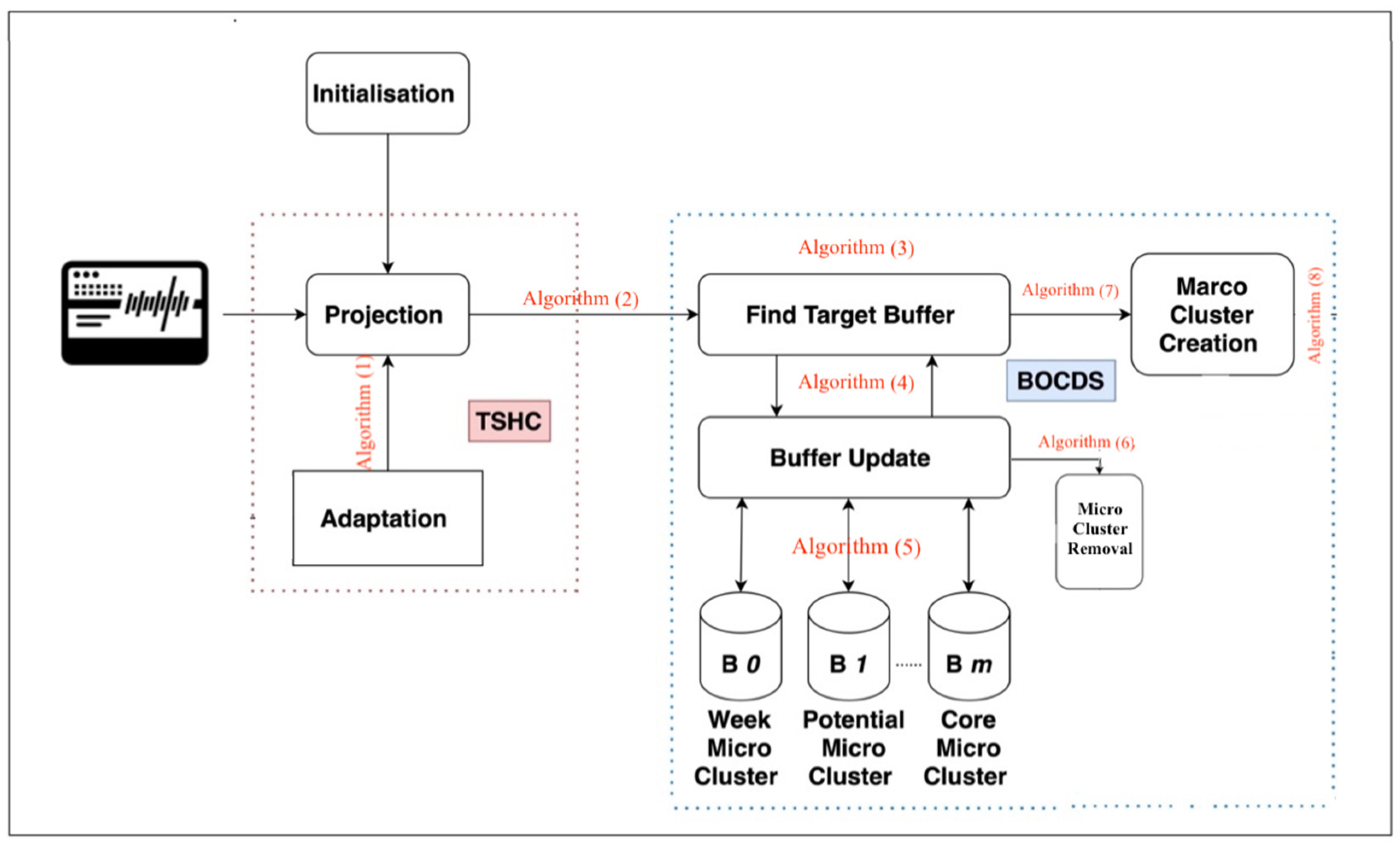
3.3. Algorithm Operation

A block diagram of the proposed algorithm is depicted in Figure 3. It receives the data stream. The data stream is fed into a projection sub-block which has the responsibility of reducing the resolution using quantization. An adaptation of this block is carried out using TSHC.

3.4. Developed Algorithms

This section presents the development of a novel algorithm named (BOCEDS-TSHC). It has the core of BOCEDS with an addition algorithm named tempo spatial hyper cube (TSHC). It is developed as an extension that augments the existing BOCEDS (or any similar density-based online stream clustering) to provide high cluster efficiency within evolving data streams respectively. The developed TSHC algorithm is an add-on to a single-phase clustering algorithm that assists in generating clusters from evolving data streams in a fully online manner. It can work independently or jointly with an existing clustering algorithm such as BOCEDS. Again, using them with the BOCEDS core can be regarded as a new clustering algorithm designated as BOCEDS-TSHC. We present the developed TSHC in the subsequent section.

3.4.1. Temporal Spatial Hyper Cube (TSHC)

The hyper-cube is a quantization level that is supposed to map various values to one value in each coordinate to reduce the resolution of data storing and eliminate the effect of slight changes that do not influence the meaning of the data (type of filtering). Two aspects will feature the cube in this study; the first one is the heterogeneity, and the second is its dynamicity. The goal of the heterogeneity is to handle the heterogeneous data of the stream. The purpose of dynamicity is to handle the evolution of the data according to the values of its features or coordinates.

The cube is calculated based on an algorithm as an adaptive hyper temp-spatial cube, and it works as the pseudocode provided by Algorithm 1. After receiving new points of the data, the algorithm starts with an initial resolution of the grid. It keeps incrementing at each dimension sequentially until obtaining the least resolution containing enough points for clustering. The algorithm can be observed as incremental neighborhood expanding for tempo-spatial hyper-cube (TSHC).

The goal of TSCH is to change the values of the quantization or the cube granularities every time new data arrived in the buffer to enable an adaptive cube with respect to both time and spatial arrangement of points. The approach uses a step of increment of the cube from initial grid values toward the converged value based on checking the condition that the number of points in one hyper-cube (or grid) should not be lower than a certain threshold. In other words, the condition of $min\left(\mathrm{NumPoints}\right)> \mathrm{cellThreshold}$ indicates the convergence case with meeting the constraint. The increment of the cube in any dimension is constrained by the inequality given in Equation (1) which assures that the increment in any dimension should not lead to exceeding the number of points than half the amount in the buffer.

$$q\left(i\right)+delta\ast max\left(B\left(:,i\right)\right)<=max(\frac{B\left(:,i\right)}{2})$$

(1)

Algorithm 1: Tempo Spatial Hyper Cube

Input:    (1) B: Data Buffer.    (2) q0: Initial quantization level.    (3) Delta: step size.    (4) outliersThreshold.    (5) cellThreshold. Output:    Q = [q1, q2, …qm]: the quantization levels where m is the number of dimensions.   1-  start algorithm   2-  initialization:      notConverged ← true      Q ← q0.      openDimensions ← 1:m.      NumPoints ← [].   3-  while notConverged do   4-    use Q to build set of hyper-cubes that contains all data points in B.   5-    for each hyper cube do   6-    calculate the number of points inside it and add it to NumPoints array.   7-    end for   8-    remove outlierscells which its NumPoints < outliersThreshold.   9-    if min(NumPoints) > cellThreshold then   10-  converged = 1 break   11-  end if   12-  chose random dimension i from openDimensions   13-  if q(i) + delta * max(B(:, i)) <= max(B(:, i)/2 then   14-  q(i) = q(i) + delta * max(B(::i)).   15-  else   16-  remove i from openDimensions.   17-  end if   18-  end while   19-  1 return Q   20-  end algorithm

3.4.2. BOCEDS-TSHC

The first added component to BOCEDS is the tempo spatial hyper-cube (TSHC) which is aimed to enable dynamic changing of the cube granularity. The pseudocode of the algorithm is presented in Algorithm 2. It accepts the data stream, initial quantization level, step size, outlier threshold, cell threshold, the ratios of calculating $R_{max}$, R_min. The output of the algorithm is the clustering result as well as the anomaly detection. The algorithm starts with an initialization of the various variables. Next, the data inside the buffer are used for finding the best cube granularity using TSHC. Next, a loop of data processing for clustering is conducted if new points arrive. At each iteration, the algorithm searches for the target micro-cluster using Algorithm 5, update the micro-cluster using Algorithm 6, update the energy of CMC, and assign CMC to macro-clusters using Algorithm 7. Each of these operations is called based on a separate algorithm that will be explained in the subsequent sub-sections.

Algorithm 2: TSHC BOCEDS

Input:   (1) Data: data stream.   (2) q0: Initial quantization level.   (3) Delta: step size.   (4) outliersThreshold.   (5) cellThreshold.   (6) RmaxRatio: the ratio to calculate $R_{max}$ from Q.   (7) RminRatio: the ratio to calculate Rmin from Rmax   (8) B: buffer Output:   Clusters: the clustering result for each data point in B.   Detected Anomaly: the Anomaly data detected in the stream   1- start algorithm   2- initialization:       endOfStream ← false       Q ← TSHC(B, q0, Delta, outliersThreshold, cellThreshold).       Rmax ← RmaxRatio ∗ norm(Q)       Rmin ← RminRatio ∗ Rmax       iniate: CMCs, PMCs, WMCs “types of micro clusters”       Tc ← 1       G ← graph()       Clusters ← []   3- while ¬ endOfStream do   4- B ← data(T c)   5- for each data piont Xi in B do   6-  T ← searchForTargetMC (Xi, Rmin, Rmax, CMCs, PMCs, WMCs) Algorithm 3   7-  if T == [] then   8-   create a new PMC   9-  else   10-    update the micro-clusters using Algorithm 4   11-   end if   12-    update Energy of CMC using Algorithm 5   13-   end if   14-   Clusters ← assignToMacroClusters (G, CMC, Clusters)   15- Tc ← Tc + 1   16-   if Tc ≥ size(data) then   17-    endOfStream←true   18-   end if   19- end while   20- end algorithm

3.4.3. BOCEDS Micro-Cluster Searching

The goal of micro-cluster searching which is shown in Algorithm 3 is to find the closest target struct to add an existing point $x_i$. There are three types of structs, namely, CMCs, which indicate a core micro-cluster set; PMCs, which indicate a potential micro-cluster set; and WMCs, which indicate a weak micro-cluster set. The output is the corresponding struct where the point is added after updating it. For the searching, Equation (6) is used which indicates having a distance of the point from the struct to its center smaller than the radius of the struct.

$$d\left(X_i,C\right)<R$$

(2)

The searching follows priority by looking at the WMCs first, PMCs second and CMCs last. Hence, the result will be either one of these structs types or an empty set when the condition of $d\left(X_i,C\right)<R$ is not applied.

Algorithm 3: BOCEDS Micro-Cluster Searching

Input:   (1) Xi: Data point   (2) CMCs: core micro-cluster set   (3) PMCs: potential micro-cluster set   (4) WMCs: weak micro-cluster set Output:    T: the Micro-cluster that contains Xi.    1- start algorithm    2- initalization:      T ← []    3- Find a weak micro-cluster Q that satisfied Equation (2).    4- if Q not empty then    5-     T ← Q          Go to Ret    6- end if    7- Find a potential micro-cluster Q that satisfied Equation (2).    8- if Q not empty then    9-     T ← Q          Go to Ret    10-  end if    11-  Find a core micro-cluster Q that satisfied Equation (2).    12-  if Q not empty then    13-      T ← Q             Go to Ret    14-  end if    15-  Ret:Return T    16-  end algorithm

3.4.4. BOCEDS Micro-Cluster Update

The goal of the micro-cluster update is to perform two functionalities: The first one is incrementing the number of points for T by 1 as it is shown in the Equation (7)

$$\mathrm{Local} \mathrm{density}, N_{t+1}=N_t+1$$

(3)

the first one is to decide whether the newly arrived data point $x_i$ will cause converting its target T to a CMC. This is accomplished when the condition in Algorithm 4 line 3 is satisfied. In this case, then the radius will be updated and the energy will be assigned to 1 as it is shown in lines 5 and 6 as it is shown in Equation (8):

$$\mathrm{Radius}, R_{t+1}=min\left(\left[R_t+\left\{\frac{2\times d\left(X_{t+1},C_t\right)}{R_t}-1\right\}\times \frac{1}{ \mathrm{Decay} }\right],R_{max}\right)$$

(4)

On the other side, when the data point already belongs to MC then the radius and the energy will be updated as it is shown in Algorithm 6 lines 8 and 9 as it is shown in Equation (9):

$$\mathrm{Energy}, E_{t+1}=E_t+\left\{\frac{R_t-d\left(X_{t+1},C_t\right)}{R_t}\right\}\times \frac{1}{ \mathrm{Decay} }$$

(5)

The last thing to do is to check whether the data point belongs to the shell as it is given in Algorithm 6 line 12. In this case, the number of points in the shell, as well as the center, are updated using Equations (10) and (11).

$$N_{t+1}^{\prime }=N_t^{\prime }+1$$

(6)

$$\mathrm{Center}, C_{t+1}^k=\frac{\left(N_{t+1}^{\prime }-1\right)\times C_t^k+X_{t+1}^k}{N_{t+1}^{\prime }}$$

(7)

The output of the algorithm is an updated CMC, PMC, or WMC. The next stage is to check whether moving micro-clusters from one buffer to another is needed. This is given in the next sub-section.

Algorithm 4: BOCEDS Micro-Cluster Update

Input:   (1) Xi: Data point   (2) CMCs: core micro-cluster set   (3) PMCs: potential micro-cluster set   (4) WMCs: weak micro-cluster set   (5) T: the Micro-cluster that contains Xi Output:   (1) CMCs:core micro-cluster set   (2) PMCs:potential micro-cluster set   (3) WMCs:weak micro-cluster set    1- start algorithm    2- Update the local density (Nt) of T using Equation (3).    3- if [(T ∈ PMCs) ∧ (Nt+1 = Thdensity)] ∨ (T ∈ WMCs) then    4-   CMCs=CMCs U T    5-   Update the radius (Rt+1) of the micro-cluster (T) using Equation (4).    6-   Et+1 ← 1    7- else if T ∈ MC core then    8-   Update the radius (Rt+1) of the micro-cluster (T) using Equation (4).    9-   Update the energy (Et+1) of the micro-cluster (T) using Equation (5).    10-  end if    11-  d ← distance (Xi, T.Center)    12-  If $\frac{R_{t+1}}{2}$ < d ≤ Rt+1, then    13-    Update the number of data points in the shell region (Nt+1) of the micro-cluster (T) using Equation (10).    14-    Update the center (Ct+1) of the micro-cluster (T) using Equation (7).    15-    Update Cluster Graph using Algorithm 5    16-  end if    17-  end algorithm

3.4.5. BOCEDS Moving Weak Micro-Clusters to a Buffer

The pseudocode of converting weak micro-cluster is presented in Algorithm 5. As it is shown, it accepts the two types of micro-cluster, namely, CMCs and WMCs in addition to decay. The output is the update of each CMC and WMC. The pseudocode starts with the energy of all CMCs with the value of $\frac{1}{Decay}$. Afterwards, for each T in CMCs, the energy is checked whenever the energy is lower than 0, and T will be removed from all CMCs and added to WMCs. When T is removed from CMCs, it is energy is set to 0.5. The next step after converting the CMCs to WMCs is to check inside WMCs and PMCs for an update on micro-cluster removal which is provided in the next sub-section.

Algorithm 5: BOCEDS Moving Weak Micro-Clusters to A Buffer

Input:   (1) CMCs: core micro-cluster set   (2) WMCs: weak micro-cluster set   (3) Decay: the decaying period Output:   (1) CMCs: core micro-cluster set   (2) WMCs: weak micro-cluster set    1- start algorithm    2- Reduce an energy of $\frac{1}{Decay }$ from all CMCs    3- for each T in CMCs do    4-   if T.Energy ≤ 0 then    5-    T.Edges ← []    6-    remove T from all CMCs edges T.M ← 0    7-    Remove T from CMCs T.Energy ← 0.5    8-    WMCs = WMCs U T    9-   end if   10-   end for   11-   end algorithm

3.4.6. BOCEDS Micro-Cluster Removal

The pseudocode of micro-cluster removal is presented in Algorithm 6. The inputs are PMCs, WMCs, and decay, and the output is PMCs and WMCs. The algorithm starts by reducing the energy with the value o $\frac{1}{Decay}$ for all micro-clusters inside WMCs. Next, for each micro-cluster in WMCs, the energy is checked and when it is lower than 0 the micro-cluster is removed from WMCs. In addition, the energy of all micro-clusters inside PMCs is checked and when it reaches the value of 0 or lower, then the micro-cluster is removed.

Algorithm 6: BOCEDS Micro-Clusters Removal

Input:   (1) PMCs: potential micro-cluster set   (2) WMCs: weak micro-cluster set   (3) Decay: the decaying period Output:   (1) PMCs: potential micro-cluster set   (2) WMCs: weak micro-cluster set    1- start algorithm    2- Reduce an energy of $\frac{1}{Decay }$ from all WMCs    3- for each W in WMCs do     4-   if T.Energy ≤ 0 then    5-    Remove W from WMCs    6-   end if    7- end for    8- Reduce an energy of $\frac{1}{Decay }$ from all PMCs    9- for each P in PMCs do     10-    if T.Energy ≤ 0 then    11-     Remove P from PMCs    12-    end if    13-  end for    14-  end algorithm

3.4.7. BOCEDS Update Cluster Graph

The update of a micro-cluster graph is based on checking the intersecting distance between the micro-clusters. Next, the value of the intersecting distance $d^{\prime }$ which is calculated based on the radius $R$ and $R^{\prime }$ of the two micro-clusters using Equation (12) is compared with the distance between them $d$ and when the distance $d^{\prime }$ is lower than $d$ then an edge is added between them and the graph is updated as it is shown in the pseudocode in Algorithm 7.

$$d^{\prime }=\{\begin{array}{c}R+{\frac{R}{2}}^{\prime }\hspace{1em}\hspace{1em}, \mathrm{if} R\ge R^{\prime }\\ R^{\prime }+\frac{R}{2}\hspace{1em}\hspace{1em}, \mathrm{if} R^{\prime }>R\end{array}$$

(8)

Algorithm 7: BOCEDS Update Cluster Graph

Input:   (1) CMCs: core micro-cluster set   (2) T: A core micro cluster that has been generated or modified   (3) G: clustering graph Output:   (1) CMCs: core micro-cluster set   (2) G: clustering graph    1- start algorithm    2- for each C in CMCs do    3-   d ← Euclideandistance(T.c, C.c)    4-   d′ ← intersectingdistance(T, C) from Equation (8)    5-   if d ≤ d′ then    6-     T.EL = T.EL ∪ Edge (T, C)    7-     C.EL = C.EL ∪ Edge (T, C)    8-   end if    9- end for     10- if any micro-cluster edge list has changed then     11-    Set a new number of macro-clusters throughout the graph.     12- end if     13- end algorithm

4. Results and Discussions

The developed clustering algorithm is implemented using MATLAB R2021a.

A series of experiments have been executed on five datasets including two real and three synthetic datasets to measure the performance of the developed BOCDES-TSHC algorithm and compare it with four benchmark clustering algorithms. The characteristics of the datasets used in the experiments are as detailed below in

Table 2. Datasets Characteristics.

Dataset Name	Number of Records	Number of Classes		Number of Features	Type	Range
DNA.mat	6006	2		1	double	[0.1, 1]
				2	double	[0, 1]
Spiral.mat	6012	2		1	double	[−0.4, 1]
				2	double	[−0.4, 0.6]
LandSat	Number	Meaning		Number of records	Type	Range
	1	red soil		1072	Integer	[0, 255]
	2	cotton crop		479
	3	grey soil		961
	4	damp grey soil		415
	5	soil with vegetation stubble		470
	6	very damp grey soil		1038
KDD Cup’99	Number of records		Attributes		Type of Attacks
	495020		42		21

. Every experiment was repeated five times using different data points every time. The performance of the developed BOCDES-TSHC algorithm is evaluated using two types of evaluation namely, quality and efficiency. Quality evaluation includes (anomaly detection ratio, rand index, adjusted rand index, and normalized mutual information) and efficiency evaluation includes (memory usage and computational cost).

4.1. Quality Evaluation

4.1.1. Anomaly Detection Ratio (ADR)

This measure is calculated based on the number of correct anomalies detected samples over the total number of anomaly samples. ARD has been used in evaluating the anomaly detection ratio in studies such as [28].

$$ADR=\frac{CAS}{Total Anomaly Samples}$$

(9)

where $CAS$ indicates the correct anomaly detected samples.

The results of the anomaly detection ratio are presented for the various datasets in Figure 4. As it is shown in the figure, TSHC has accomplished high values for a median of ADR, nearly 1.00 for both KDD datasets which were superior to the benchmark, and a median close to 0.95 for traffic data which is equivalent to the benchmark of BOCEDS and BOCEDS inc. The only two datasets that caused an inferior performance of TSHC are DNA and Landsat. This shows a general superiority of TSHC in terms of ADR. The reason for some cases where the benchmarks were superior is the nature of the data. For example, in LandSat the results of ADR were low for all algorithms of BOCEDS, and TSHC, while CEDAS and MuDi-Stream have accomplished around 0.4 of ADR which is interpreted by the type of anomaly of LandSat which is not detectable by the buffer-based structure of BOCEDAS and our developed algorithms. On the other side, the anomaly of DNA was detectable by BOCEDS with a level higher than 0.8 but their nature did not require the dynamic awareness that exists in TSHC which makes the prediction slightly lower than BOCEDAS and BOCEDS Inc.

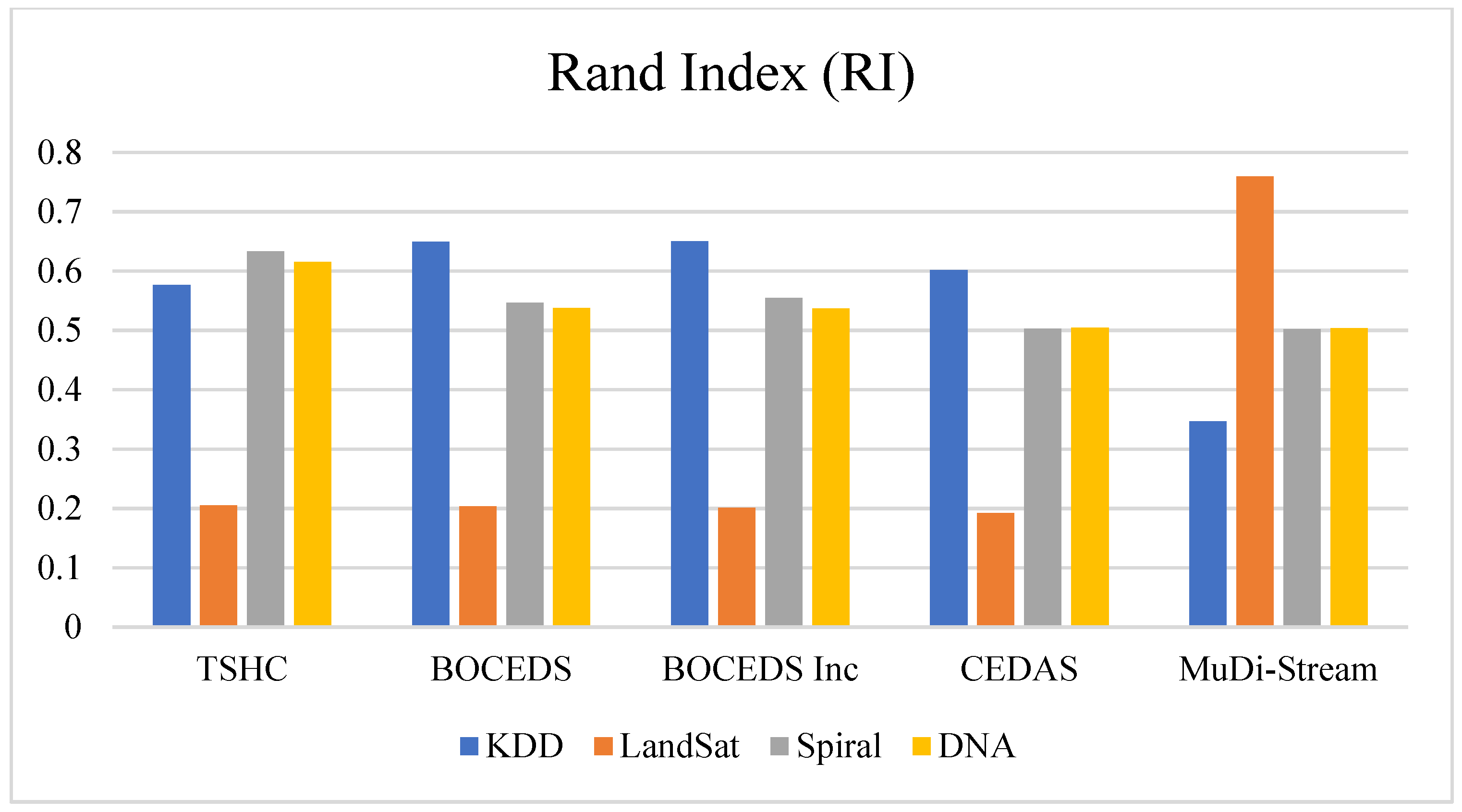
4.1.2. Rand Index (RI)

The Rand index is a widely used indicator that is primarily used to evaluate clustering. Additionally, it is used to assess density-based data stream clustering algorithms [16]. It quantifies the agreement between two partitions, i.e., how similar the clustering results are to the ground truth. The Rand index is defined as the following: [16,29,30].

$$\mathrm{Rand\; Index} =\frac{\left|TP\right|+\left|TN\right|}{\left|TP\right|+\left|TN\right|+\left|FP\right|+\left|FN\right|}$$

(10)

RI is one of the most known indices for measuring the similarity between two partitions and has been widely used in various studies.

The rand index outcomes for several datasets are visualized in Figure 5. As it is presented in the figure, the median of RI for TSHC in both DNA and spiral datasets is 0.62 and 0.64 respectively, which are higher than the benchmarks. The only two datasets that caused an inferior performance of TSHC are KDD and Landsat. The lower performance obtained in LandSat is by the nature of data that is less dynamic and did not need a buffer. Structuring and detecting the different clusters is more from a density perspective which has enabled MuDi to get better performance.

4.1.3. Adjusted Rand Index (ARI)

The adjusted rand index (ARI) is a development of the rand index (RI). It is recommended as the index of choice when comparing two partitions in a clustering analysis with a variable number of clusters. The adjusted rand index (ARI) is defined as the following:

$$ARI=\frac{\left(\begin{array}{c}n\\ 2\end{array}\right)\left(\left|TP\right|+\left|TN\right|\right)-\left[\left(\left|TP\right|+\left|FN\right|\right)\left(\left|TP\right|+\left|FP\right|\right)+\left(\left|Fp\right|+\left|TN\right|\right)\left(\left|FN\right|+\left|TN\right|\right)\right]}{{\left(\begin{array}{c}n\\ 2\end{array}\right)}^2-\left[\left(\left|TP\right|+\left|FN\right|\right)\left(\left|TP\right|+\left|FP\right|\right)+\left(\left|FP\right|+\left|TN\right|\right)\left(\left|FN\right|+\left|TN\right|\right)\right]}$$

(11)

Generally, an ARI value ranges from 0 to 1. The index value is 1 only if a partition is identical to the intrinsic structure, and it is close to 0 if the partition is random. ARI is utilized in a variety of research to evaluate data stream clusterings [16,29,30].

The adjusted rand index for the various datasets is illustrated in Figure 6. As presented in the figure, the median of ARI for TSHC in DNA, spiral, and Landsat datasets were 0.22, 0.1, 8, and 0.08 which is higher than BOCEDS, BOCEDS Inc., CEDAS, and MuDi-Stream, respectively. The values of ARI were almost zeros for LandSat due to the nature of this data which has a highly non-organized structure and makes it difficult to be partitioned into groups based on a non-supervised algorithm.

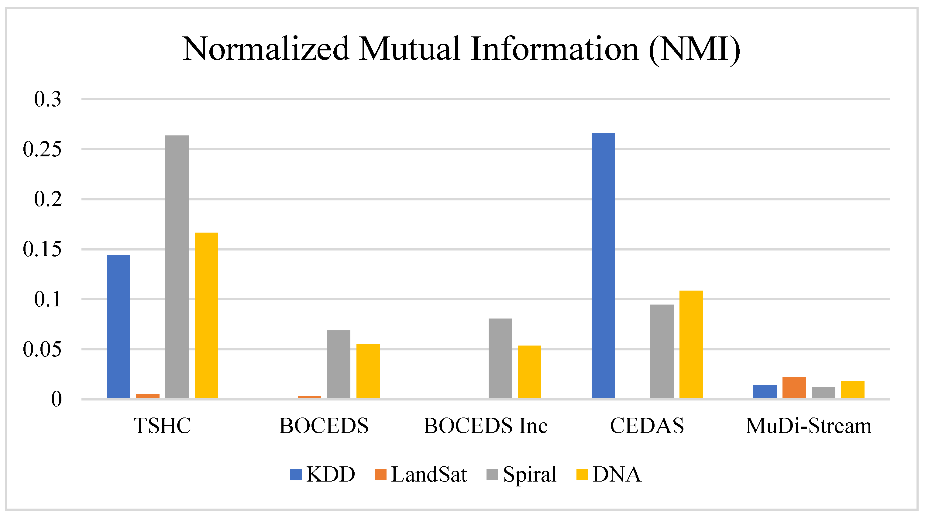
4.1.4. Normalized Mutual Information (NMI)

The normalized mutual information (NMI) is a well-known information-theoretic statistic that indicates the degree of similarity between two clusterings. Indeed, to make a trade-off between clustering quality and clustering density. NMI can also be used when the number of classes is not equal to the number of clusters. NMI(C, G) is defined as the normalized mutual information:

$$\mathrm{NMI}(C,G)=\frac{{\sum }_i{\sum }_j\frac{n_{ij}}{n}\log \frac{n\ast n_{ij}}{a_i\ast b_j}}{\sqrt{{\sum }_i{a}_i\ast \log \left(\frac{a_i}{n}\right)\ast {\sum }_j{b}_j\ast \log \left(\frac{b_j}{n}\right)}}$$

(12)

Normalized mutual information is a measurement for determining the quality of clustering. It reaches its maximum value of 1 only when the two sets of labels correspond perfectly. NMI has been used to evaluate data stream clustering in a variety of research [14,15,23,31].

In Figure 7, the findings of normalized mutual information are provided for the multiple datasets. As illustrated in the figure, TSHC has accomplished high values for a median of NMI, nearly 0.32 for both DNA datasets which were superior to the benchmark, and a median close to 0.29 for the Spiral dataset, which is higher than the benchmark of BOCEDS, BOCEDS Inc., CEDAS and MuDi-Stream. The only two datasets that caused an inferior performance of TSHC are Landsat and KDD. Similarly, all algorithms have failed in providing good NMI for LandSat which is interpreted by the nature of the data.

4.2. Efficiency Evaluation

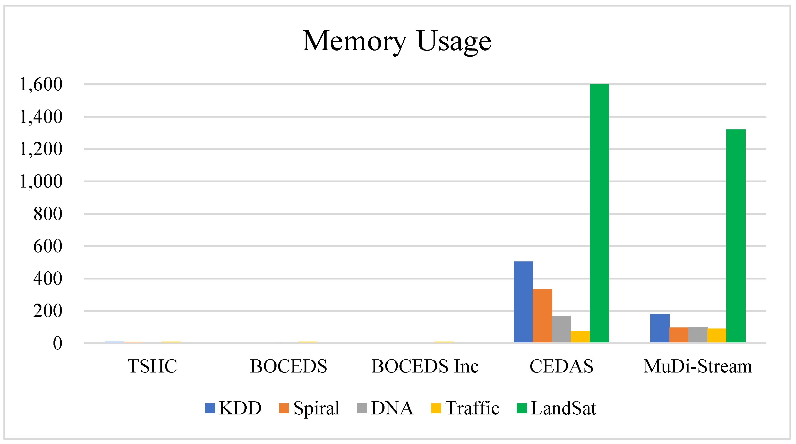
The efficiency evaluation is used for evaluating the efficiency of the developed BOCDES TSHC-ATI-SD algorithm, which includes memory usage and computational cost, which is performed using four different datasets as given below:

4.2.1. Memory Usage

The memory usage is calculated based on the number of core-mini clusters generated from each of the algorithms. As given in Figure 8, it is found that CEDAS and MuDi-Stream were the most in terms of memory usage compared with the other algorithms including ours and BOCEDS. This applies to all datasets. Another observation is that CEDAS has generated a higher value of memory usage compared with MuDi-Stream. This shows that adding extra buffer clusters to CEDAS is effective in reducing its original memory usage and making it efficient in terms of memory such as BOCEDS, BOCEDS Inc., and TSHC.

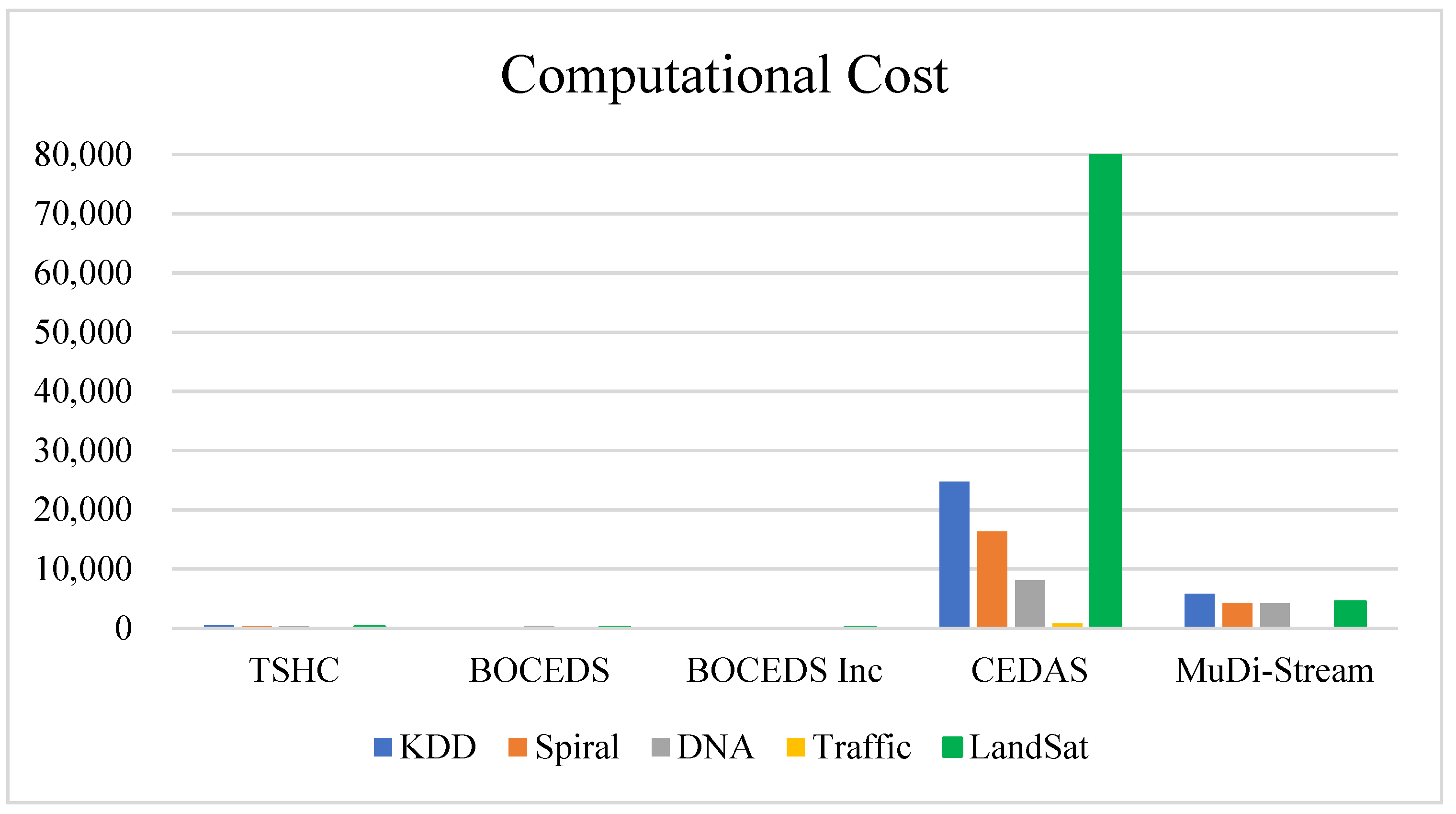
4.2.2. Computational Cost

Visualizing Figure 9, it is found that computational cost is also correlated with memory usage. Hence, CEDAS is the worst in terms of the computational cost followed by MuDi-Stream while all BOCEDS, BOCEDS Inc, and TSHC are the least in terms of the computational cost. This is also clearer when we visualize the bar chart that is provided in Figure 8. We interpret this with light memory consumption which requires low effort for data processing and low computational cost.

Theoretically, clustering algorithms are required to have a fixed and small memory usage as well as low computational cost for the entire process of the clustering data stream. Memory usage is calculated based on the number of Micro-clusters generated by an algorithm. The more the algorithm requires to generate Micro-cluster till it reaches its final clusters the more memory usage it requires. In evaluating the memory usage of a clustering algorithm, the developed algorithm uses the core mini-clusters that are stored for calculating the results of clustering as a measure of memory usage. Similarly, the computational cost is calculated based on the time the algorithm requires to perform the mathematical calculation of the distance to the Core-cluster. Thus, the more the algorithm perform mathematical calculation the more computational cost it requires. In evaluating the computational cost of a clustering algorithm, the developed algorithm uses the number of calling the distance function as an indicator for computational complexity.

5. Finding and Summary

The results and analysis of the developed BOCEDS TSHC algorithm have been discussed in detail based on two real (KDD Cup’99 and LandSat) and three synthetics (DNA, Spiral, and Traffic) datasets. Both real and syntactic datasets are used for the evaluation of the developed algorithm. The real and synthetic datasets are selected from the most used dataset in the literature. They vary in size, cluster count, and density. In addition, simulated traffic data is generated using MATLAB R2021a to is generated to simulate the evolving behavior in the data for an urban environment scenario. On the other hand, four well-known quality evaluation metrics including (anomaly detection ratio, rand index, adjusted rand index, and normalized mutual information) are selected to demonstrate the superiority of the developed algorithm. Additionally, two efficiency evaluation metrics namely (memory usage and computational cost) are used to illustrate the efficiency of the developed algorithm.

The quality evaluation of the developed algorithm to generate clusters in evolving data streams has been evaluated using both real and syntactic datasets. The result demonstrates the superiority of the developed BOCEDS TSHC algorithm in handling evolving data streams using the recursive and dynamic update for adaptive quantization of arrived data when they are projected to the clustering space. Similarly, regarding the efficiency evaluation, the results illustrate the developed BOCEDS TSHC algorithm’s superiority in both memory usage and computational cost, where the developed algorithm is found to be using less memory and computational cost. As a result, more applicability to real-world data stream scenarios.

In short, the developed BOCEDS TSHC algorithm clearly shows the best performance in terms of quality and efficiency evaluation. BOCEDS TSHC is an effective and efficient clustering algorithm in clustering evolving data streams.

6. Conclusions

This study developed an online clustering algorithm for handling evolving data streams with anomaly detection called BOCDES TSHC. The developed algorithm can handle the challenges of clustering evolving data streams by enabling temporal and spatial projection. The tempo-spatial hyper cube (TSHC) is used to increase the degree of freedom in data summarization by adding extra dimensions. When TSHC is combined with Buffer-based Online Clustering for Evolving Data Stream (BOCEDS), a superior evolving data stream clustering technique is created. The developed BOCEDS TSHC clustering algorithm outperformed the baseline algorithms in most clustering measures, according to evaluations based on both real-world and synthetic datasets. Yet, this research opens some research issues to be solved in the future, extending the tempo spatial Cartesian grid with a polar grid to handle the curvy shape of clusters might be a future work extension to the algorithm. However, this depends on the type of data and the clusters that result from the data. For some data, curvy clusters with circular shapes are likely to occur which makes the polar representation more efficient in terms of memory. Moreover, adding more buffers to the core of clustering (BOCEDS) such as potential anomaly buffers and potential outliers. This makes the algorithm more careful before deciding to remove a potential outlier.

References

1. Yu, K.; Shi, W.; Santoro, N. Designing a streaming algorithm for outlier detection in data mining—An incrementa approach. Sensors 2020, 20, 1261. [Google Scholar] [CrossRef] [PubMed] [Green Version]
2. Degirmenci, A.; Karal, O. Efficient Density and Cluster Based Incremental Outlier Detection in Data Streams. Inf. Sci. 2022, 607, 901–920. [Google Scholar] [CrossRef]
3. Al-Amri, R.; Murugesan, R.K.; Alshari, E.M.; Alhadawi, H.S. Toward a Full Exploitation of IoT in Smart Cities: A Review of IoT Anomaly Detection Techniques. In International Conference on Emerging Technologies and Intelligent Systems; Lecture Notes in Networks and Systems; Springer: Cham, Switzerland, 2022; Volume 322, pp. 193–214. [Google Scholar] [CrossRef]
4. Märzinger, T.; Kotík, J.; Pfeifer, C. Application of hierarchical agglomerative clustering (Hac) for systemic classification of pop-up housing (puh) environments. Appl. Sci. 2021, 11, 11122. [Google Scholar] [CrossRef]
5. Zubaroğlu, A.; Atalay, V. Data Stream Clustering: A Review; Springer: Amsterdam, The Netherlands, 2020. [Google Scholar]
6. Al-amri, R.; Murugesan, R.K.; Man, M.; Abdulateef, A.F. A Review of Machine Learning and Deep Learning Techniques for Anomaly Detection in IoT Data. Appl. Sci. 2021, 11, 5320. [Google Scholar] [CrossRef]
7. Habeeb, R.A.A.; Nasaruddin, F.; Gani, A.; Hashem, I.A.T.; Ahmed, E.; Imran, M. Real-time big data processing for anomaly detection: A Survey. Int. J. Inf. Manag. 2019, 45, 289–307. [Google Scholar] [CrossRef] [Green Version]
8. Carnein, M.; Trautmann, H. Optimizing Data Stream Representation: An Extensive Survey on Stream Clustering Algorithms. Bus. Inf. Syst. Eng. 2019, 61, 277–297. [Google Scholar] [CrossRef] [Green Version]
9. Maia, J.; Junior, C.A.S.; Guimarães, F.G.; de Castro, C.L.; Lemos, A.P.; Galindo, J.C.F.; Cohen, M.W. Evolving clustering algorithm based on mixture of typicalities for stream data mining. Future Gener. Comput. Syst. 2020, 106, 672–684. [Google Scholar] [CrossRef]
10. Manzoor, E.; Lamba, H.; Akoglu, L. xStream: Outlier Detection in Feature-Evolving Data Streams. In Proceedings of the 24th ACM SIGKDD International Conference on Knowledge Discovery & Data Mining, New York, NY, USA, 19–23 August 2018. [Google Scholar] [CrossRef]
11. Anandharaj, A.; Sivakumar, P.B. Anomaly Detection in Time Series data using Hierarchical Temporal Memory Model. In Proceedings of the 2019 3rd International conference on Electronics, Communication and Aerospace Technology (ICECA), Coimbatore, India, 12–14 June 2019; pp. 1287–1292. [Google Scholar] [CrossRef]
12. Gottwalt, F.; Chang, E.; Dillon, T. CorrCorr: A feature selection method for multivariate correlation network anomaly detection techniques. Comput. Secur. 2019, 83, 234–245. [Google Scholar] [CrossRef]
13. Munir, M.; Siddiqui, S.A.; Dengel, A.; Ahmed, S. DeepAnT: A Deep Learning Approach for Unsupervised Anomaly Detection in Time Series. IEEE Access 2019, 7, 1991–2005. [Google Scholar] [CrossRef]
14. Hyde, R.; Angelov, P.; MacKenzie, A.R. Fully online clustering of evolving data streams into arbitrarily shaped clusters. Inf. Sci. 2017, 382–383, 96–114. [Google Scholar] [CrossRef] [Green Version]
15. Islam, M.K.; Ahmed, M.M.; Zamli, K.Z. A buffer-based online clustering for evolving data stream. Inf. Sci. 2019, 489, 113–135. [Google Scholar] [CrossRef]
16. Amini, A.; Saboohi, H.; Herawan, T.; Wah, T.Y. MuDi-Stream: A multi density clustering algorithm for evolving data stream. J. Netw. Comput. Appl. 2016, 59, 370–385. [Google Scholar] [CrossRef]
17. Ghorabaee, M.K.; Zavadskas, E.K.; Turskis, Z.; Antucheviciene, J. A new combinative distance-based assessment (CODAS) method for multi-criteria decision-making. Econ. Comput. Econ. Cybern. Stud. Res. 2016, 50, 25–44. [Google Scholar]
18. Škrjanc, I.; Ozawa, S.; Ban, T.; Dovžan, D. Large-scale cyber attacks monitoring using Evolving Cauchy Possibilistic Clustering. Appl. Soft Comput. J. 2018, 62, 592–601. [Google Scholar] [CrossRef]
19. Chenaghlou, M.; Moshtaghi, M.; Leckie, C.; Salehi, M. Online Clustering for Evolving Data Streams with Online Anomaly Detection; Springer International Publishing: Cham, Switzerland, 2018; Volume 10938. [Google Scholar]
20. Islam, M.K.; Ahmed, M.M.; Zamli, K.Z. I-CODAS: An improved online data stream clustering in arbitrary shaped clusters. Eng. Lett. 2019, 27, 752–776. [Google Scholar]
21. Salort Sanchez, C.; Tudoran, R.; Al Hajj Hassan, M.; Bortoli Stefano Brasche, G.; Baumbach, J.; Axenie, C. An Online Incremental Clustering Framework for Real-Time Stream Analytics. In Proceedings of the 2019 18th IEEE International Conference On Machine Learning And Applications (ICMLA), Boca Raton, FL, USA, 16–19 December 2019; pp. 1480–1485. [Google Scholar] [CrossRef]
22. Roa, N.B.; Travé-Massuyès, L.; Grisales-Palacio, V.H. DyClee: Dynamic clustering for tracking evolving environments. Pattern Recognit. 2019, 94, 162–186. [Google Scholar] [CrossRef] [Green Version]
23. Tareq, M.; Sundararajan, E.A.; Mohd, M.; Sani, N.S. Online Clustering of Evolving Data Streams Using a Density Grid-Based Method. IEEE Access 2020, 8, 166472–166490. [Google Scholar] [CrossRef]
24. Islam, M.K.; Sarker, B. An Online Clustering Approach for Evolving Data-Stream Based on Data Point Density. In Proceedings of the International Conference on Emerging Technologies and Intelligent Systems, Al Buraimi, Oman, 25–26 June 2021; pp. 105–115. [Google Scholar]
25. Xia, Y.; Fang, J.; Chao, P.; Pan, Z.; Shang, J.S. Cost-effective and adaptive clustering algorithm for stream processing on cloud system. Geoinformatica 2021, 1–21. [Google Scholar] [CrossRef]
26. Tareq, M.; Sundararajan, E.A.; Harwood, A.; Bakar, A.A. A Systematic Review of Density Grid-Based Clustering for Data Streams. IEEE Access 2022, 10, 579–596. [Google Scholar] [CrossRef]
27. Albertini, M.K.; de Mello, R.F. Estimating data stream tendencies to adapt clustering parameters. Int. J. High Perform. Comput. Netw. 2018, 11, 34–44. [Google Scholar] [CrossRef]
28. Zheng, J.; Qu, H.; Li, Z.; Li, L.; Tang, X. An irrelevant attributes resistant approach to anomaly detection in high-dimensional space using a deep hypersphere structure. Appl. Soft Comput. 2022, 116, 108301. [Google Scholar] [CrossRef]
29. Carnein, M.; Trautmann, H. evoStream—Evolutionary Stream Clustering Utilizing Idle Times. Big Data Res. 2018, 14, 101–111. [Google Scholar] [CrossRef]
30. Yeh, C.C.; Yang, M.S. Evaluation measures for cluster ensembles based on a fuzzy generalized Rand index. Appl. Soft Comput. 2017, 57, 225–234. [Google Scholar] [CrossRef]
31. Xu, L.; Ye, X.; Kang, K.; Guo, T.; Dou, W.; Wang, W.; Wei, J. DistStream: An Order-Aware Distributed Framework for Online-Offline Stream Clustering Algorithms. In Proceedings of the 2020 IEEE 40th International Conference on Distributed Computing Systems (ICDCS), Singapore, 29 November–1 December 2020; pp. 842–852. [Google Scholar] [CrossRef]
Figure 1. Flowchart of the Developed Methodology.
Applsci 12 06523 g001
Figure 2. Visualization of DNA and Spiral Datasets.
Applsci 12 06523 g002
Figure 3. Online Clustering Algorithm developed.
Applsci 12 06523 g003
Figure 4. Anomaly Detection Ratio Comparison Using KDDCup’99, Landsat, Spiral, DNA, and Traffic Datasets.
Applsci 12 06523 g004
Figure 5. Rand Index Comparison Using KDDCup’99, Landsat, Spiral, and DNA Datasets.
Applsci 12 06523 g005
Figure 6. Adjusted Rand Index Comparison Using KDDCup’99, Landsat, Spiral, and DNA Datasets.
Applsci 12 06523 g006
Figure 7. Normalized Mutual Information Comparison Using KDDCup’99, Landsat, Spiral, and DNA Datasets.
Applsci 12 06523 g007
Figure 8. Memory Usage Comparison using KDDCup’99, Landsat, Spiral, DNA, and Traffic Datasets.
Applsci 12 06523 g008
Figure 9. Computational Cost Comparison using KDDCup’99, Landsat, Spiral, DNA, and Traffic Datasets.
Applsci 12 06523 g009