Dynamic Modeling of a Flexible-Link Flexible-Joint System with Tip Mass Considering Stiffening Effect

Abstract

This paper presents the dynamic model of a flexible-link, flexible-joint manipulator system with a considerable stiffening effect of the flexible link. A gripper, along with tip mass, is attached at one end of the flexible link. By employing the extended Hamilton’s principle, a nonlinear governing equation of motion is derived along with several boundary constraints. Under the assumption of small deformation in free vibration, a simplified motion equation is deduced to determine the natural frequencies of the mechanical system. Four parameters of the system are selected to carry out the sensitivity study on frequency. The results show that the second frequency mainly depends on the mass of tip payload. Moreover, the third frequency is significantly affected by the moment inertia of tip payload. Regarding the constant angular motion, the finite element method is adopted to analyze the dynamic model by considering the stiffening effect. The frequency results are obtained which show a higher stiffness of the Single Flexible-link Flexible-joint (SFF) system with the angular velocity increasing. The influence of three factors (i.e., payload mass, length of the flexible link, and angular velocity) on the fundamental natural frequencies are discussed, which show instinct characteristics of the flexible manipulator system.

1. Introduction

Commercial robotics composed of multiple links have been widely applied in several industrial domains. For serial robots with rigid links, they are usually invented to maintain their high repeated accuracy with heavy mechanical structures. This feature leads to a dynamic motion of the mechanical system in a relatively limited working speed because of the large mass-inertia of bulky structures. With the development of new composite materials and advanced manufacturing methods, the mechanical flexibility of robotic manipulators has attracted many researchers with the merits of high-speed motion, large-scale manipulation, and low manufacturing cost [1,2,3,4,5,6].

One of the principal issues for using flexible-link manipulators with rotational actuators is to develop the accurate dynamic model of flexible systems, which had been studied by researchers and engineers for over 20 years [7,8,9,10,11,12]. The ultimate performance of model-based controllers is mainly dependent on the accuracy of dynamic system models [13]. The particular feature of a flexible link is denoted as the capability of allowing a transversal deflection away from the predefined undeformed link. Regarding the flexible beam modeling methods, there are two well-known approaches, namely the Timoshenko beam theory [14] and the Euler–Bernoulli beam theory [7,9,12,15,16,17,18]. The Euler–Bernoulli beam theory is widely used with the assumption of neglecting both the shear deformation and rotary mass moment of inertia. A potential technique to reduce the influence of shear deformation during a large motion proposed in [17,18] is to use two parallel cable units on both sides of the flexible beam. In addition, the Euler–Bernoulli beam theory is sufficient to predict the dynamic performance of slender composite beams with a slenderness ratio larger than 20 [19]. New materials for flexible systems can be applied in the design of soft exoskeletons, which have been reviewed in [20]. The governing equations of motion of a flexible link with tip payload can be modeled using six methods [21]. Hamilton’s principle [7,10,12,22], Lagrange equations [21], and Newton–Euler equations [23] are often applied for developing a dynamic system model of a mechanical system. A dynamic modeling of a single-link flexible robot with a tip payload using the Newton–Euler formulation was addressed by Rakhsha [23]. Natural frequencies and corresponding modal shapes were obtained for a study case in accordance with those in the literature. An accurate dynamic model of a flexible-link system can be expressed by Partial Differential Equations (PDEs) with a set of boundary conditions. Furthermore, a closed-form characteristic equation is yielded from the PDEs of flexible-link systems, which can be utilized to study the influence of structure design parameters on vibration features [9]. As for discrete flexible-link models, the Finite Element Method (FEM) is applied to transform PDEs into Ordinary Differential Equations (ODEs) for the purpose of investigating the vibration characteristics of a flexible-link system in the time and frequency domains [22]. Another method, the Assumed Mode Method (AMM) [24], is exploited by replacing the accurate shape modals with some shape modals of classical flexible beam models (e.g., clamped-free beams, clamped-clamped beams, clamped-roller beams, and roller-free beams). Generally, FEM with more degrees of freedom produces more precise results than when using AMM. However, FEM costs more time to calculate the results of flexible-link systems in comparison to AMM.

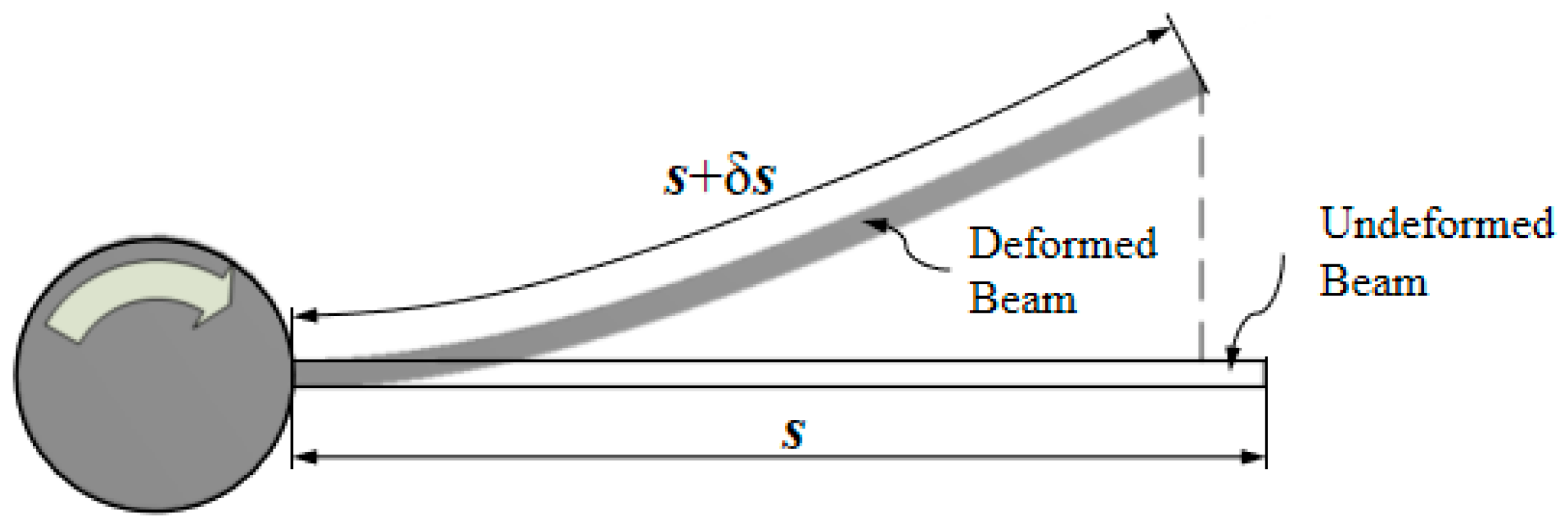
Moreover, it is worth noting that the foreshortening (geometric stiffening or stress stiffness in [8], as shown in Figure 1) of the flexible link should be considered in the dynamic modeling for rotating structures [21,25,26,27], while it is negligible for small angular velocity [7]. In [21], Piedœuf studied the dynamics models of a flexible beam using different methods based on the assumptions by neglecting the foreshortening effect. Al-Qaisia in [24] developed four mathematical models to discuss the stiffening effect of rotating flexible links. These models are denoted as the Consistent Model (CM), Potential energy Model (PM), Kinetic energy Model (KM), as well as the Kinetic and Potential Model (KPM). A conclusion is obtained that CM, without considering the stiffening effect, leads to static instability at a critical angular velocity, while other three models are highly improved by considering the stiffening effect. Among PM, KM, and KPM, the effect of the rotating speed on the vibration behavior of all modes was discussed according to a series of simulation results. The main target of this paper is to develop the dynamic modeling of a Single Flexible-link Flexible-joint (SFF) manipulator by introducing the stiffening effect in the potential energy model, which was neglected in [10,12].

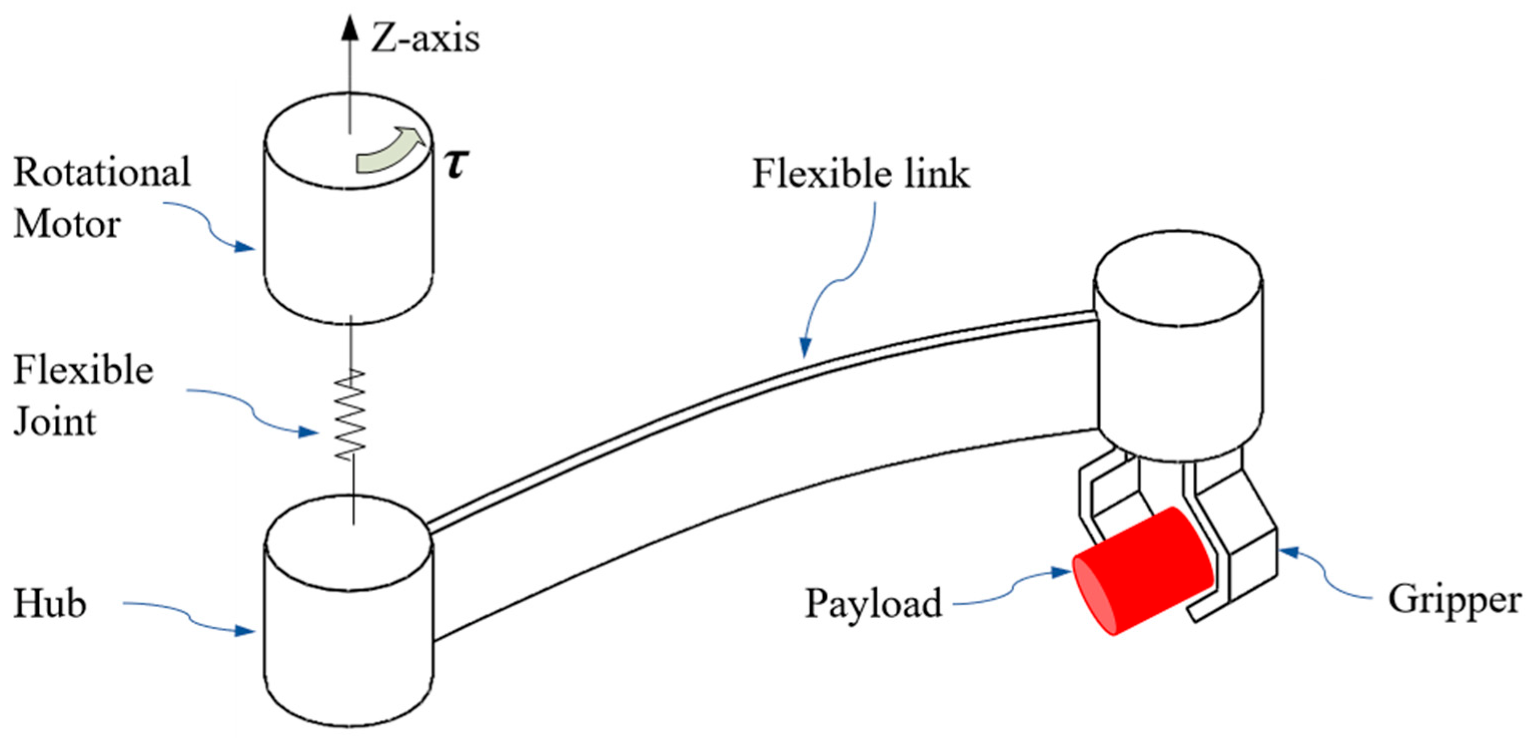
Except for the link flexibility, there is another type of flexibility related to rotational joints which is also important in mechanical systems. A single flexible-link, flexible-joint manipulator investigated in the paper is illustrated in Figure 2. A rotational actuator connects the hub through a flexible joint, and a flexible beam is clamped at the hub with a tip payload attached at the distal end of the beam. As the counterpart of the SFF mechanism, a single flexible-link, rigid-joint mechanism and a single rigid-link, flexible-joint mechanism had also been utilized when performing the mode analysis [10], which showed several differences among these three mechanisms. In order to study the influence of the rotational stiffness of the flexible joint on the vibration features, a sensitivity index is introduced from the closed-form characteristic equation of the flexible-link system. The results confirmed that the joint flexibility of the rotational actuator has a significant effect on the system frequencies [9].

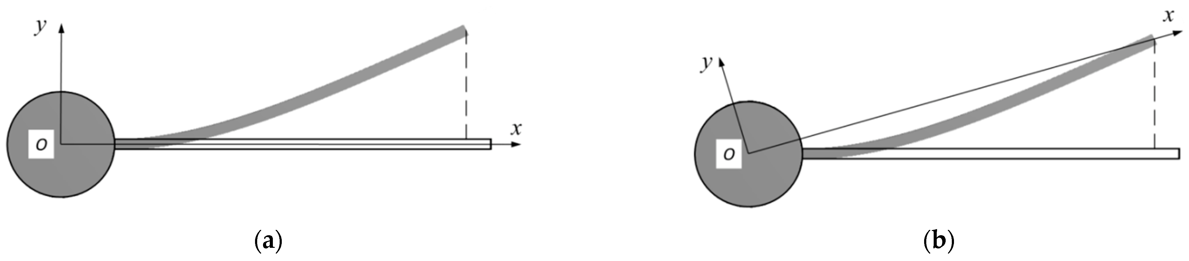
In the process of modeling slender links, the position of the curvilinear points on flexible links is depicted in the relative coordinate systems. For the convenience of kinematic analysis, two typical coordinate systems illustrated in Figure 3 are defined as Virtual Link Coordinate System (VLCS) [28] and Tangential Coordinate System (TCS). Coordinate systems for flexible systems are also mentioned in [8] as pseudo-clamped, pseudo-pinned, and pseudo-pinned-pinned systems, where the pseudo-clamped reference frame is the same as TCS and pseudo-pinned-pinned to VLCS. As shown in Figure 3, the largest transversal deflection occurs at one end of a slender link for TCS, while it is represented near the middle point of the link for VLCS. Additionally, in VLCS, the deformation of the flexible link at both ends are assigned as zero. In comparison, in TCS, it is clearer to describe the transversal deformation of a slender link along with several boundary constraints. Therefore, TCS is employed in the present paper to facilitate the dynamic modeling of SFF systems in the following sections.

In this paper, the relative coordinate system used for modeling the flexible link is defined as TCS. A rotational motor exerts a torque τ to make the hub rotate. A flexible joint connects the motor and a hub as a pure torsional spring. A payload is exactly attached to the distal end of the flexible link without any deviation for simplicity. The proximal end of the flexible link is clamped by the hub. The governing equation of motion as PDE is deduced by the Hamilton principle in Section 2. The stiffening effect is considered in the dynamic modeling. Natural frequencies and mode shapes of an SFF system are discussed based on the dynamic modeling in Section 3. The stiffening effect of the flexible link system with constant rotational velocity is investigated in Section 4. Conclusions and remarks are included in Section 5.

2. Dynamic Modeling

As shown in Figure 2, a typical SFF system includes a rotational actuator, a flexible joint, a hub, a slender link, and a tip payload. J_m, θ_m, and τ are used to denote the moment of inertia of the motor, the angular displacement of the actuator, and the torque applied to the rotational actuator. The flexible joint is considered as a purely torsional spring with constant stiffness k. The hub is assumed as a cylinder with a diameter R and the inertia J_h. The flexible link with uniform cross-sections is described with bending stiffness EI and a length L having density per unit length ρ. The payload is attached to the flexible link with the mass m_p and the moment of inertia J_p. The motion of the slender link is limited in the horizontal plane regardless of gravity. 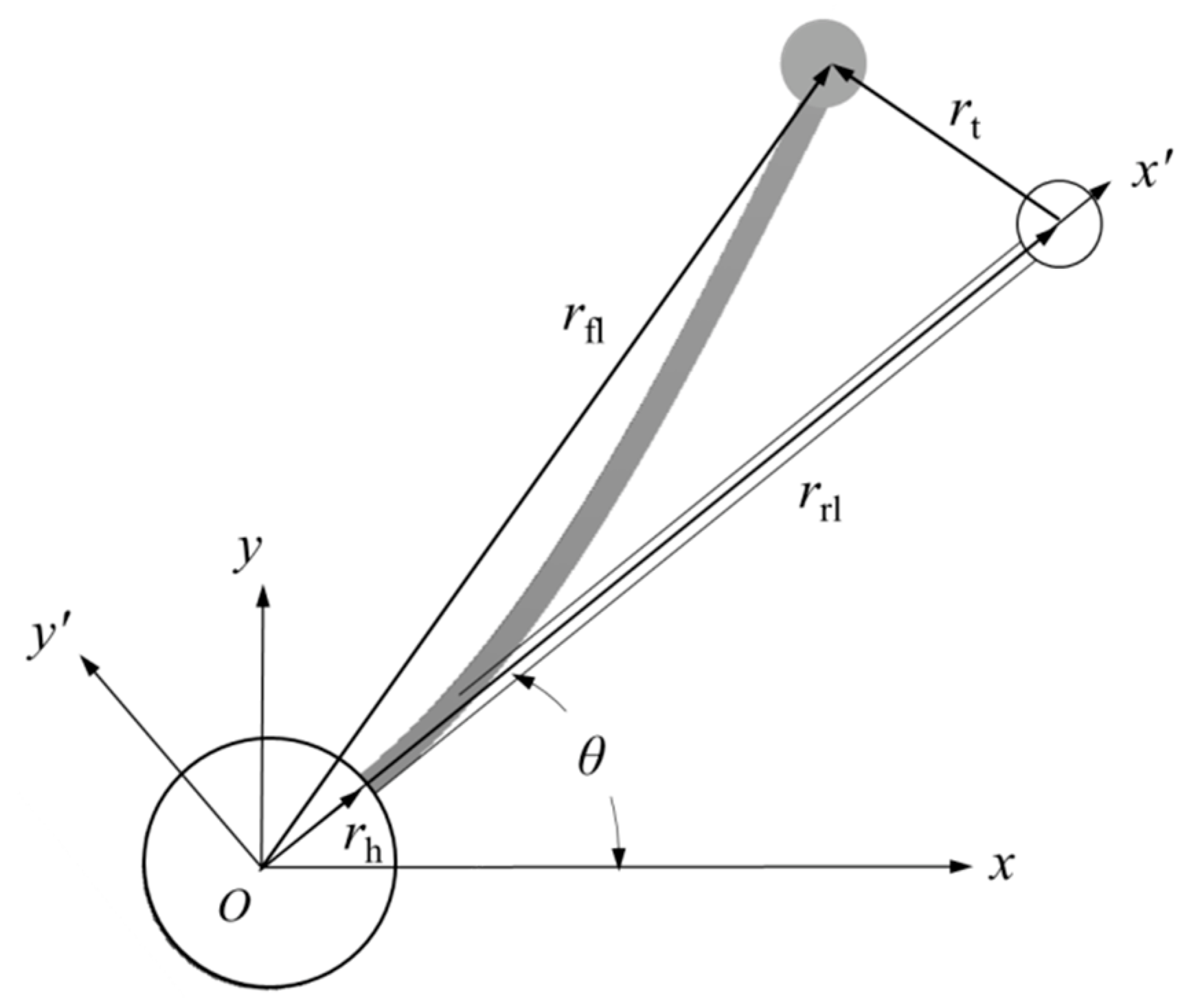$O-xy$ frame is denoted as the inertial frame of the SFF. The relative coordinate system $O-x’y’$ is referred to as the TCS with the axis $x’$ along the undeformed link. θ represents the angular displacement of the slender link in the inertial frame in Figure 4.

The location of curvilinear points on the flexible link consists of a rigid location of the undeformed link and a transversal deflection due to the flexibility. The rigid location vector of a point is expressed as$r_{\mathrm{rl}}$. The transversal deflection vector is denoted as$r_{\mathrm{t}}={\left[u,v\right]}^{\mathrm{T}}$, which is related to the location of the curvilinear point s along the link and time.$r_{\mathrm{h}}$ is given as the location vector pointing to the proximal end of the link. Therefore, the location of the point on the link is obtained as

$$r_{\mathrm{fl}}=r_{\mathrm{h}}+r_{\mathrm{rl}}+r_{\mathrm{t}}$$

(1)

The original location of the point with respect to the inertial frame is denoted as$\left(x,0\right)$. The rotational matrix from the relative coordinate frame to the inertial global frame is denoted as

$$T=\left[\begin{array}{cc}\cos \theta & -\sin \theta \\ \sin \theta & \cos \theta \end{array}\right].$$

(2)

By combining Equations (1) and (2), the location vector is transferred as

$$r_{\mathrm{fl}}=\left[\begin{array}{cc}\cos \theta & -\sin \theta \\ \sin \theta & \cos \theta \end{array}\right]\left(\left[\begin{array}{c}x\\ 0\end{array}\right]+\left[\begin{array}{c}u\\ v\end{array}\right]\right),$$

(3)

Based on the assumption of the inextensible flexible link, the following constraint equation is obtained as

$${\left(1+\frac{\partial u}{\partial \mathrm{s}}\right)}^2+{\left(\frac{\partial v}{\partial \mathrm{s}}\right)}^2=1.$$

(4)

To incorporate the stiffening effect in an SFF system, the potential energy of the system is composed of the potential energy of the flexible link $V_{\mathrm{L}}$ due to bending, the energy V_A caused by the axial shortening and the inertial force, and the potential energy of the torsional spring. The expression of $V_{\mathrm{L}}$ can be deduced as

$$V_{\mathrm{L}}=\frac{EI{\lambda }^3}{2}{{\displaystyle \int }}_0^1\left[{\left(\frac{{\partial }^{2}v}{\partial {\zeta }^2}\right)}^2+{\lambda }^2{\left(\frac{{\partial }^{2}v}{\partial {\zeta }^2}\right)}^2{\left(\frac{\partial v}{\partial \zeta }\right)}^2\right]\mathrm{d}\zeta .$$

(5)

The virtual work due to the inertial force and the link foreshortening displacement is obtained as

$$V_{\mathrm{A}}=-\frac{{\dot{\theta }}^2}{2}{{\displaystyle \int }}_0^1\left[m_{\mathrm{p}}\left(R+L\right)+\frac{\rho L^2\left(1-{\zeta }^2\right)}{2}+\rho LR\left(1-\zeta \right)\right]\left[\lambda {\left(\frac{\partial v}{\partial \zeta }\right)}^2\right]\mathrm{d}\zeta .$$

(6)

Moreover, the potential energy of the torsional spring is

$$V_{\mathrm{S}}=\frac{k}{2}{\left({\theta }_{\mathrm{m}}-\theta \right)}^2.$$

(7)

Thus, the entire potential energy of the system is expressed as

$$V=V_{\mathrm{L}}+V_{\mathrm{A}}+V_{\mathrm{S}}.$$

(8)

In the present paper, the kinetic energy of the slender link is expressed as

$$T_{\mathrm{L}}=\frac{\rho L}{2}{{\displaystyle \int }}_0^1{\left(\frac{\partial r_{\mathrm{fl}}}{\partial t}\right)}^{\mathrm{T}}\left(\frac{\partial r_{\mathrm{fl}}}{\partial t}\right)\mathrm{d}\zeta .$$

(9)

Considering $x=\zeta L+R$, the following formulation can be obtained as

$$T_{\mathrm{L}}=\frac{\rho L}{2}{{\displaystyle \int }}_0^1\left\{\begin{array}{c}{\left(\frac{\mathrm{d}\theta }{\mathrm{dt}}\right)}^2\left[{\left(\zeta L+R\right)}^2+u^2+2u\left(\zeta L+R\right)+v^2\right]+\\ 2\left(\frac{\mathrm{d}\theta }{\mathrm{dt}}\right)\left[\left(\mathsf{\zeta }L+R\right)\left(\frac{\partial v}{\partial t}\right)+u\left(\frac{\partial v}{\partial t}\right)-\left(\frac{\partial u}{\partial t}\right)v\right]+{\left(\frac{\partial v}{\partial t}\right)}^2+{\left(\frac{\partial u}{\partial t}\right)}^2\end{array}\right\}\mathrm{d}\zeta .$$

(10)

Similarly, the kinetic energy of the tip payload is introduced as

$$T_{\mathrm{P}}=\frac{m_{\mathrm{p}}}{2}{\left({\left.\frac{\partial r_{\mathrm{fl}}}{\partial t}\right|}_{s=L}\right)}^{\mathrm{T}}\left({\left.\frac{\partial r_{\mathrm{fl}}}{\partial t}\right|}_{s=L}\right)+\frac{J_{\mathrm{p}}}{2}{\left(\frac{\mathrm{d}\theta }{\mathrm{d}t}+{\left.\frac{{\partial }^{2}v}{\partial s\partial t}\right|}_{s=L}\right)}^2.$$

(11)

Thus, the entire kinetic energy of the flexible system is yielded as

$$T=\frac{1}{2}{J}_{\mathrm{m}}{\left(\frac{\mathrm{d}{\theta }_{\mathrm{m}}}{dt}\right)}^2+\frac{1}{2}{J}_{\mathrm{h}}{\left(\frac{\mathrm{d}\theta }{\mathrm{d}t}\right)}^2+T_{\mathrm{L}}+T_{\mathrm{P}}.$$

(12)

The virtual work exerted by the rotational actuator torque is $\mathsf{\delta }W=\tau \mathsf{\delta }{\theta }_{\mathrm{m}}$.

As mentioned in the introduction, there are three methods to develop the dynamic equations of motion of the flexible link system. In the following deduction, the extended Hamilton’s principle is applied as

$${{\displaystyle \int }}_{t_1}^{t_2}\left(\delta T-\delta V+\delta W\right)\mathrm{d}t=0.$$

(13)

By taking into account that $\mathsf{\delta }{\theta }_{\mathrm{m}},\mathsf{\delta }\theta ,\mathsf{\delta }v, \mathsf{\delta }{\left.\left(\frac{\partial v}{\partial \mathrm{s}}\right)\right|}_{\mathrm{s}=\mathrm{L}}\mathrm{and} {\left.\mathsf{\delta }v\right|}_{\mathrm{s}=\mathrm{L}}$ are separate variations, the expressions of $A_1,A_2,A_3,A_4, \mathrm{and} A_5$ are equal to zero (for more details in Appendix A). Therefore, the dynamical model of a flexible-link, flexible-joint manipulator with tip mass considering the stiffening effect is formulated as

$$J_{\mathrm{m}}\left(\frac{{\mathrm{d}}^2{\theta }_{\mathrm{m}}}{\mathrm{d}{t}^2}\right)+\tau -k\left({\theta }_{\mathrm{m}}-\theta \right)=0,$$

(14)

$$EI\frac{{\partial }^{4}v}{\partial s^4}+{\left(\frac{\mathrm{d}\theta }{\mathrm{d}t}\right)}^2\left[m_{\mathrm{p}}L+\frac{\rho \left(L^2-s^2\right)}{2}\right]\left(\frac{{\partial }^{2}v}{\partial s^2}\right)+\rho \left[s\left(\frac{{\mathrm{d}}^2\theta }{\mathrm{d}{t}^2}\right)+v{\left(\frac{\mathrm{d}\theta }{\mathrm{d}t}\right)}^2+\left(\frac{{\partial }^{2}v}{\partial t^2}\right)\right]=0,$$

(15)

$$\begin{gathered} J_{\mathrm{p}}\left(\frac{{\mathrm{d}}^2\theta }{\mathrm{d}{t}^2}+{\left.\frac{{\partial }^{3}v}{\partial s\partial t^2}\right|}_{s=L}\right)+{{\displaystyle \int }}_0^1\left\{\rho L\left({\zeta }^2{L}^2+v^2\right)+\left[m_{\mathrm{p}}+\frac{\rho L\left(1-{\zeta }^2\right)}{2}\right]{\left(\frac{\partial v}{\partial \zeta }\right)}^2\right\}\left(\frac{{\mathrm{d}}^2\theta }{\mathrm{d}{t}^2}\right)\mathrm{d}\zeta + \\ {m}_{\mathrm{p}}\left(L^2+{\left.v^2\right|}_{s=L}\right)\left(\frac{{\mathrm{d}}^2\theta }{\mathrm{d}{t}^2}\right)+{{\displaystyle \int }}_0^1\rho \zeta L^2\left(\frac{{\partial }^{2}v}{\partial t^2}\right)\mathrm{d}\zeta +m_{\mathrm{p}}L{\left.\left(\frac{{\partial }^{2}v}{\partial t^2}\right)\right|}_{s=L}+ \\ {{\displaystyle \int }}_0^1\rho Lv\left(\frac{\partial v}{\partial t}\right)\mathrm{d}\zeta \left(\frac{\mathrm{d}\theta }{\mathrm{d}t}\right)+m_{\mathrm{p}}{\left.v\right|}_{s=L}{\left.\left(\frac{\partial v}{\partial t}\right)\right|}_{s=L}\left(\frac{\mathrm{d}\theta }{\mathrm{d}t}\right)+k\left({\theta }_{\mathrm{m}}-\theta \right)=0, \end{gathered}$$

(16)

$${\left.EI\left(\frac{{\partial }^{2}v}{\partial s^2}\right)\right|}_{s=L}+J_{\mathrm{p}}\left(\frac{{\mathrm{d}}^2\theta }{\mathrm{d}{t}^2}+{\left.\frac{{\partial }^{3}v}{\partial s\partial t^2}\right|}_{s=L}\right)=0,$$

(17)

$$m_{\mathrm{p}}L\left(\frac{{\mathrm{d}}^2\theta }{\mathrm{d}{t}^2}\right)+m_{\mathrm{p}}{\left.\left(\frac{{\partial }^{2}v}{\partial t^2}\right)\right|}_{s=L}-EI{\left.\left(\frac{{\partial }^{3}v}{\partial s^3}\right)\right|}_{s=L}=0,$$

(18)

with two boundary constraint conditions at s = 0,

$${\left.v\right|}_{s=0}^{}=0,{\left.\frac{\partial v}{\partial s}\right|}_{s=0}^{}=0.$$

(19)

3. Natural Frequency Analysis of SFF

The dynamic characteristics of an SFF mechanism consists of the natural frequency of the flexible system in the frequency domain and the dynamic response in time domain. Assuming that the lateral deformation $v$, $\theta$, and ${\theta }_{\mathrm{m}}$ are separable in space and time, which are introduced as

$$v\left(s,t\right)=\Psi \left(s\right)\sin \left(\omega t\right),\hspace{1em}\hspace{1em}\theta =\Theta \sin \left(\omega t\right),\hspace{1em}\hspace{1em}{\theta }_{\mathrm{m}}={\Theta }_{\mathrm{m}}\sin \left(\omega t\right),$$

(20)

where $\Psi \left(\mathrm{s}\right),\Theta , \mathrm{and} {\Theta }_{\mathrm{m}}$ are parameters in space. By the substitution of Equation (20) into Equations (14) and (15), the expressions are given as below when the external torque $\tau =0$,

$$k\Theta =\left(k-{\omega }^2{J}_{\mathrm{m}}\right){\Theta }_{\mathrm{m}},$$

(21)

$$\begin{gathered} EI\frac{{\partial }^4\Psi }{\partial s^4}\sin \left(\omega t\right)+{\left(\frac{\mathrm{d}\theta }{\mathrm{d}t}\right)}^2\left[m_{\mathrm{p}}L+\frac{\rho \left(L^2-s^2\right)}{2}\right]\left(\frac{{\partial }^2\Psi }{\partial s^2}\right)\sin \left(\omega t\right)+ \\ \rho \left[-s\left(\Theta {\omega }^2\right)\sin \left(\omega t\right)+\Psi \left(s\right)\sin \left(\omega t\right){\left(\frac{\mathrm{d}\theta }{\mathrm{d}t}\right)}^2-\Psi \left(s\right){\omega }^2\sin \left(\omega t\right)\right]=0. \end{gathered}$$

(22)

Regardless of the higher order of $\frac{\mathrm{d}\mathsf{\theta }}{\mathrm{dt}}$, it is given as

$$EI\frac{{\partial }^4\Psi \left(s\right)}{\partial s^4}-{\omega }^2\rho \left[s\Theta +\Psi \left(s\right)\right]=0.$$

(23)

Let ${\beta }^4={\omega }^2\rho /EI$, then it is simplified as

$$\frac{{\partial }^4\Psi \left(s\right)}{\partial s^4}-{\beta }^4\Psi \left(s\right)-{\beta }^{4}s\Theta =0,$$

(24)

where

$$\Psi \left(s\right)=A\sin \left(\beta s\right)+B\cos \left(\beta s\right)+\mathrm{Csinh}\left(\mathsf{\beta }\mathrm{s}\right)+\mathrm{Dcosh}\left(\mathsf{\beta }\mathrm{s}\right)-\mathsf{\Theta }\mathrm{s}.$$

(25)

Based on Equation (25) and Equations (17)–(19) can be rewritten as

$$\begin{gathered} \left[-\rho \sin \left(\beta L\right)-J_{\mathrm{p}}{\beta }^3\cos \left(\beta L\right)\right]A+\left[J_{\mathrm{p}}{\beta }^3\sin \left(\beta L\right)-\rho \cos \left(\beta L\right)\right]B \\ +\left[\rho \sin \mathrm{h}\left(\beta L\right)-J_{\mathrm{p}}{\beta }^3\cos \mathrm{h}\left(\beta L\right)\right]C+\left[\rho \cos \mathrm{h}\left(\beta L\right)-J_{\mathrm{p}}{\beta }^3\sin \mathrm{h}\left(\beta L\right)\right]D=0, \end{gathered}$$

(26)

$$\begin{gathered} \left[m_{\mathrm{p}}\beta \sin \left(\beta L\right)-\rho \cos \left(\beta L\right)\right]A+\left[m_{\mathrm{p}}\beta \cos \left(\beta L\right)+\rho \sin \left(\beta L\right)\right]B \\ +\left[m_{\mathrm{p}}\beta \sin \mathrm{h}\left(\beta L\right)+\rho \cos \mathrm{h}\left(\beta L\right)\right]C+\left[m_{\mathrm{p}}\beta \cos \mathrm{h}\left(\beta L\right)+\rho \sin \mathrm{h}\left(\beta L\right)\right]D=0, \end{gathered}$$

(27)

$$B+D=0,$$

(28)

$$\beta A+\beta C-\Theta =0.$$

(29)

Subsequently, an additional equation is obtained from Equation (16) as

$$J_{\mathrm{p}}\Theta +J_{\mathrm{p}}{\Psi }^{\prime }\left(L\right)+\frac{\rho L^3}{3}\Theta +m_{\mathrm{p}}{L}^2\Theta +{{\displaystyle \int }}_0^{\mathrm{L}}\rho s\Psi \left(s\right)\mathrm{d}s+m_{\mathrm{p}}L\Psi \left(L\right)+J_{\mathrm{m}}{\Theta }_{\mathrm{m}}=0.$$

(30)

Based on Equations (26)–(30), the coefficients $A,B,C,D \mathrm{and} \Theta$ need to fulfill

$$\stackrel{𝚷}{\overbrace{\left[\begin{array}{c}{H}_{11}\\ H_{21}\\ H_{31}\\ 0\\ \beta \end{array},\begin{array}{c}{H}_{12}\\ H_{22}\\ H_{32}\\ 1\\ 0\end{array},\begin{array}{c}{H}_{13}\\ H_{23}\\ H_{33}\\ 0\\ \beta \end{array},\begin{array}{c}{H}_{14}\\ H_{24}\\ H_{34}\\ 1\\ 0\end{array},\begin{array}{c}0\\ 0\\ H_{35}\\ 0\\ -1\end{array}\right]}}\stackrel{{\rm X}}{\overbrace{\left[\begin{array}{c}A\\ B\\ C\\ D\\ \Theta \end{array}\right]}}=\left[\begin{array}{c}0\\ 0\\ 0\\ 0\\ 0\end{array}\right],$$

(31)

where

$$\begin{gathered} H_{11}=-\rho \sin \left(\beta L\right)-J_{\mathrm{p}}{\beta }^3\cos \left(\beta L\right),H_{12}=J_{\mathrm{p}}{\beta }^3\sin \left(\beta L\right)-\rho \cos \left(\beta L\right), \\ {H}_{13}=\rho \sin \mathrm{h}\left(\beta L\right)-J_{\mathrm{p}}{\beta }^3\cos \mathrm{h}\left(\beta L\right),H_{14}=\rho \cos \mathrm{h}\left(\beta L\right)-J_{\mathrm{p}}{\beta }^3\sin \mathrm{h}\left(\beta L\right), \\ {\mathrm{H}}_{21}={\mathrm{m}}_{\mathrm{p}}\mathsf{\beta }\sin \left(\mathsf{\beta }\mathrm{L}\right)-\mathsf{\rho }\cos \left(\mathsf{\beta }\mathrm{L}\right),{ \mathrm{H}}_{22}={\mathrm{m}}_{\mathrm{p}}\mathsf{\beta }\cos \left(\mathsf{\beta }\mathrm{L}\right)+\mathsf{\rho }\sin \left(\mathsf{\beta }\mathrm{L}\right), \\ {H}_{23}=m_{\mathrm{p}}\beta \sin \mathrm{h}\left(\beta L\right)+\rho \cos \mathrm{h}\left(\beta L\right),H_{24}=m_{\mathrm{p}}\beta \cos \mathrm{h}\left(\beta L\right)+\rho \sin \mathrm{h}\left(\beta L\right), \\ {H}_{31}=m_{\mathrm{p}}L\sin \left(\beta L\right)+J_{\mathrm{p}}\beta \cos \left(\beta L\right)+\rho {{\displaystyle \int }}_0^L\sin \left(\beta s\right)s\mathrm{d}s, \\ {H}_{32}=m_{\mathrm{p}}L\cos \left(\beta L\right)-J_{\mathrm{p}}\beta \sin \left(\beta L\right)+\rho {{\displaystyle \int }}_0^L\cos \left(\beta s\right)s\mathrm{d}s, \\ {H}_{33}=m_{\mathrm{p}}L\sin \mathrm{h}\left(\beta L\right)+J_{\mathrm{p}}\beta \cos \mathrm{h}\left(\beta L\right)+\rho {{\displaystyle \int }}_0^L\sin \mathrm{h}\left(\beta s\right)s\mathrm{d}s, \\ {H}_{34}=m_{\mathrm{p}}L\cos \mathrm{h}\left(\beta L\right)+J_{\mathrm{p}}\beta \sin \mathrm{h}\left(\beta L\right)\rho {{\displaystyle \int }}_0^L\cos \mathrm{h}\left(\beta s\right)s\mathrm{d}s, \\ {H}_{35}=\frac{\rho }{3}{L}^3+m_{\mathrm{p}}{L}^2+J_{\mathrm{p}}+\frac{\rho k{J}_{\mathrm{m}}}{\rho k-{\beta }^{4}EI{J}_{\mathrm{m}}}. \end{gathered}$$

In Equation (31), only the item H₃₅ is related to the parameters of the flexible joint and the motor. If k is extremely large, the SFF system is transformed into a Single Flexible-link Rigid-joint (SFR) system. Under this circumstance of an SFR system, it is equivalent to a cantilever beam with tip mass. To achieve the non-trivial solution of vector x in Equation (31), the determinant of matrix $\Pi$ must be equal to zero. Once finding the parameter $\beta$, the natural frequency $\omega$ is able to be calculated according to ${\beta }^4={\omega }^2\rho /EI$. To compare the results, the values of the physical parameters of the SFF manipulator are chosen with those in [12], as below in

Table 1. Geometrical and Material Parameters of an SFF manipulator.

Item	Parameter	Value	Unit
Mass density	$\rho$	0.41	$\mathrm{kg}/\mathrm{m}$
Link bending stiffness	EI	20.82	$\mathrm{N}·{\mathrm{m}}^2$
Link length	L	1	m
Motor moment of inertia	$J_{\mathrm{m}}$	173	$\mathrm{kg}·{\mathrm{m}}^2$
Stiffness of the flexible joint	$k$	624.6	$\mathrm{N}·\mathrm{m}/\mathrm{rad}$
Payload moment of inertia	$J_{\mathrm{p}}$	0.005	$\mathrm{kg}·{\mathrm{m}}^2$
Payload mass	$m_{\mathrm{p}}$	2	$\mathrm{kg}$

.

Based on the assumption of the small displacement, the natural frequencies are listed and compared in

Table 2. Comparison of Natural frequencies of an SFF manipulator (unit: rad/s).

Order	GMM [12]	Present Method
1	-	5.1486
2	19.3996	18.0539
3	91.7603	89.8060
4	217.4268	216.1903
5	465.1852	463.1632

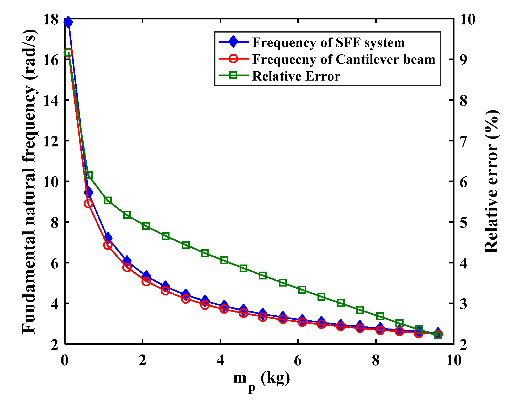
. When the order of the system model is higher, the natural frequency is closer to that with the Global Mode Method (GMM) in [12]. The natural frequencies in this paper show good agreement with the results in [12]. As mentioned in [23], the fundamental frequency of a cantilever beam of mass $m_{\mathrm{L}}$ with tip mass of $m_{\mathrm{p}}$ as

$${\omega }_1=\sqrt{\frac{3EI}{\left(m_{\mathrm{p}}+\frac{33}{140}{m}_{\mathrm{L}}\right)L^3}}.$$

(32)

By substituting of the values in Table 1, the fundamental natural frequency of the SFF system from Equation (32) is ${\omega }_1=5.4581 \mathrm{rad}/\mathrm{s}$. The value of the fundamental frequency obtained from the proposed method is $5.1486 \mathrm{rad}/\mathrm{s}$ with an error of $5.67\%$. As shown in Figure 5, the obtained fundamental frequencies from Equations (31) and (32) are well matched.

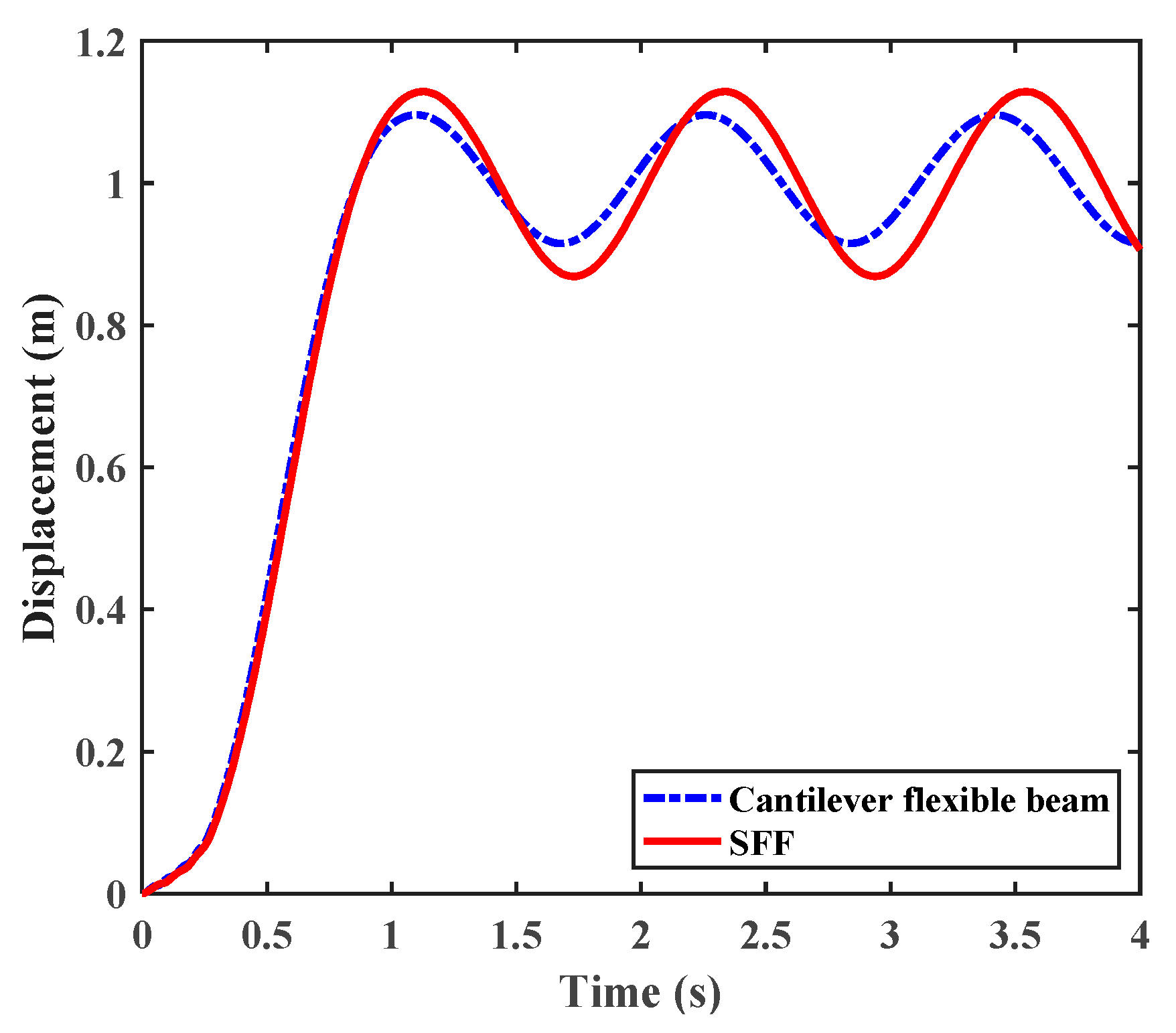
To verify the analytical results, two simulations are implemented with commercial software ANSYS. The first simulation is performed as a free vibration of a cantilever flexible beam with tip mass. The model is developed with tip mass but without the flexible joint. A flexible joint (i.e., a torsional joint) is added to the model in the second simulation. The physical parameters utilized in these two simulations follow the values in Table 1. In the first simulation, the flexible link rotates around the axis with a constant angular velocity of 1 rad/s during the period of 0~1.1 s and starts in a free vibration from 1.1 s. The fundamental frequency from the simulation is obtained as ${\mathsf{\omega }}_1^{\mathrm{c}}=2\mathsf{\pi }/1.1562=5.4343 \mathrm{rad}/\mathrm{s}$, while the frequency from Equation (39) is ${\mathsf{\omega }}_1=5.4581 \mathrm{rad}/\mathrm{s}$—very close to the result of the first simulation. In the second simulation, the fundamental frequency of the SFF system is obtained from the simulation as ${\mathsf{\omega }}_1^{\mathrm{s}}=2\mathsf{\pi }/1.21=5.19 \mathrm{rad}/\mathrm{s}$. The corresponding frequency obtained in the paper is $5. 1486 \mathrm{rad}/\mathrm{s}$, with the relative error of 0.8%. For comparison, the displacements of the top mass in these two simulations are depicted in Figure 6, where the solid line denotes the displacement of SFF system and the dashed line denotes that of the cantilever beam with tip mass.

Next, the sensitivity analysis of each parameter can be implemented to discuss the effect on the natural frequency. Four main variables are selected in a feasible range to study how the natural frequency changes.

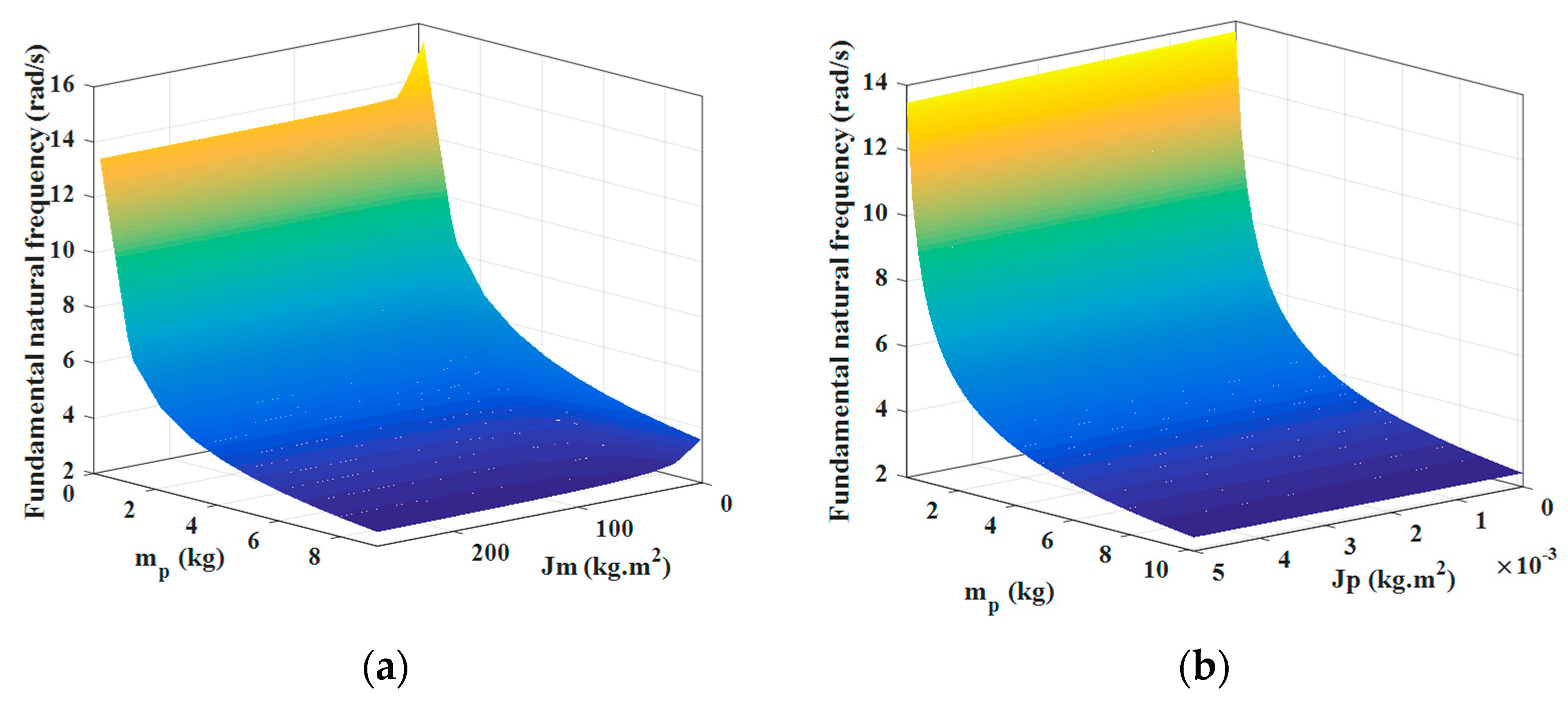
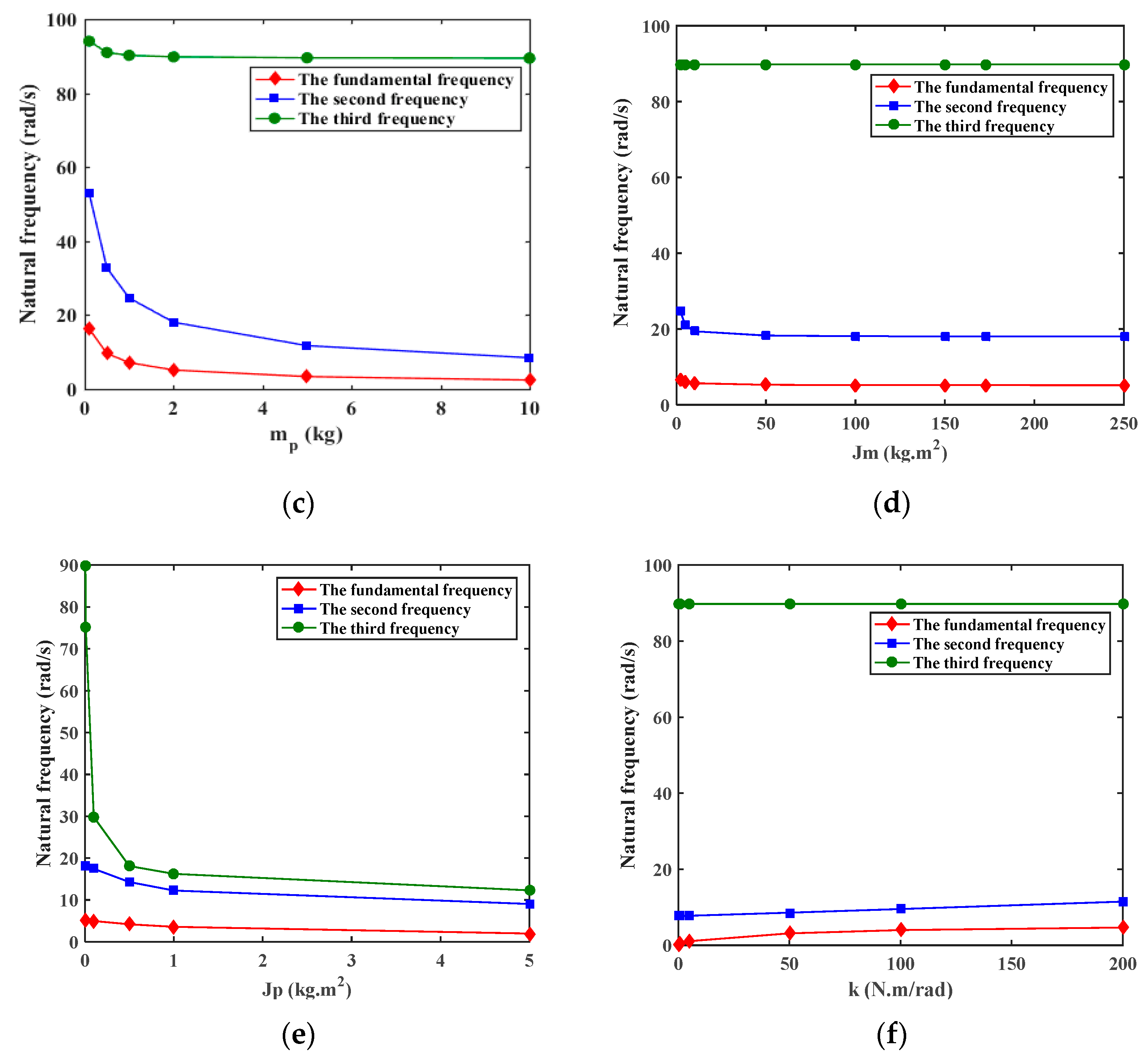
As depicted in Figure 7, the mass of the payload plays a highly important role in the fundamental natural frequency (denoted as diamond marks) of an SFF system. Furthermore, the fundamental natural frequency is less sensitive to the moment inertia of the motor. Regarding the second frequency (denoted as square marks), it mainly depends on the mass of the payload. These two conclusions are in agreement with the results reported in [10]. Additionally, the value of the third frequency is affected by the moment inertia of the tip payload, which is not discussed in [10]. Moreover, the fundamental and the second frequencies are also related to the stiffness of the flexible joint in the system. Although the numerical method can be applied to sensitivity analysis on natural frequency of the SFF, an analytical expression of natural frequency, together with the physical parameters of the SFF system, is more practical for sensitivity analysis. However, the analytical expression of natural frequency is deduced as an involved formula, which is omitted in the paper.

After determining the value of natural frequencies, the matrix $\Pi$ can be obtained by applying the frequencies. Then, the modal shape is able to be determined by employing the eigenvector of the matrix $\Pi$ with the corresponding eigenvalue equal to zero. Therefore, the exact dynamic equation of the points on the links is developed based on the modals of the SFF system.

Using the frequencies in Table 2, the modal shapes (as illustrated in Figure 8) of the flexible link are denoted as

$$\left\{\begin{array}{c}{\Psi }_1\left(\mathrm{s}\right)=27.1\sin \left({\beta }_{1}s\right)-22.24\cos \left({\beta }_{1}s\right)-25.92\sin \mathrm{h}\left({\beta }_{1}s\right)+22.33\cos \mathrm{h}\left({\beta }_{1}s\right)+s,\\ {\Psi }_2\left(s\right)=-0.0296\sin \left({\beta }_{2}s\right)+0.63\cos \left({\beta }_{2}s\right)+0.658\sin \mathrm{h}\left({\beta }_{2}s\right)-0.63\cos \mathrm{h}\left({\beta }_{2}s\right)+s,\\ {\Psi }_3\left(s\right)=-32.6\sin \left({\beta }_{3}s\right)+31.82\cos \left({\beta }_{3}s\right)+32.88\sin \mathrm{h}\left({\beta }_{3}s\right)-31.82\cos \mathrm{h}\left({\beta }_{3}s\right)+s,\\ {\Psi }_4\left(\mathrm{s}\right)=-74.83\sin \left({\beta }_{4}s\right)+75.74\cos \left({\beta }_{4}s\right)+75.01\sin \mathrm{h}\left({\beta }_{4}s\right)-75.84\cos \mathrm{h}\left({\beta }_{4}s\right)+s,\\ {\Psi }_5\left(s\right)=-169.1\sin \left({\beta }_{5}s\right)+169.1\cos \left({\beta }_{5}s\right)+169.1\sin \mathrm{h}\left({\beta }_{5}s\right)-169.1\cos \mathrm{h}\left({\beta }_{5}s\right)+s,\end{array}\right.$$

(33)

where ${\beta }_1=0.85, {\beta }_2=1.5917,{\beta }_3=3.55,{\beta }_4=5.508,{\beta }_5=8.061, \mathrm{and} s\in \left[0,L\right].$Dynamic response is achieved by truncating the nonlinear partial differential equation into the ordinary differential equations with n normalized mode shapes of the SFF system.

4. Stiffening Effect

In the previous section, the dynamic model of the SFF manipulator system is developed on a basis of the small deformation assumption in free vibration. However, the stiffening effect is highly related to its rotational velocity in Equation (15), which is neglected in Section 3. By reviewing Equation (15), the stiffening effect of the SFF system becomes more prominent when a high angular velocity is considered. To reduce the complexity of the issue, the angular velocity remains constant so that the term $\left(\frac{{\mathrm{d}}^2\theta }{\mathrm{d}{t}^2}\right)$ in Equation (15) is equal to 0. Thus, Equation (15) with a constant angular velocity is simplified as

$$EI\frac{{\partial }^{4}v}{\partial s^4}+{\left(\frac{\mathrm{d}\theta }{\mathrm{d}t}\right)}^2\left[m_{\mathrm{p}}L+\frac{\rho \left(L^2-s^2\right)}{2}\right]\left(\frac{{\partial }^{2}v}{\partial s^2}\right)+\rho \left[v{\left(\frac{\mathrm{d}\theta }{\mathrm{d}t}\right)}^2+\left(\frac{{\partial }^{2}v}{\partial t^2}\right)\right]=0.$$

(34)

After several mathematical combination manipulations, the governing equation of motion is obtained as

$$\mathrm{E}I\frac{{\partial }^{4}v}{\partial s^4}+\rho \left(\frac{{\partial }^{2}v}{\partial t^2}\right)+\varnothing \left(\Gamma \frac{{\partial }^{2}v}{\partial s^2}+\rho v\right)=0,$$

(35)

where $\varnothing ={\left(\frac{\mathrm{d}\theta }{\mathrm{d}t}\right)}^2 \mathrm{and} \Gamma =m_{\mathrm{p}}L+\frac{\rho \left(L^2-s^2\right)}{2}.$

Since Equation (35) is not able to be expressed in an explicit form, the Finite Element Method (FEM) is used in this section to analyze the natural frequency of the SFF system, considering the stiffening effect. By employing the approach mentioned in [22], the lateral deformation of the ith element is denoted as

$$v_i\left(x,t\right)={\Psi }_e\left(x\right)Q_e^i\left(t\right),$$

(36)

where ${\Psi }_e\left(x\right)$ represents a shape function of the link in terms of length x, and $Q_e\left(t\right)$is referred to as the nodal displacement with respect to time. By following the shape function defined in [12,23] with Hermite interpolation, it is written as

$${\Psi }_e\left(x\right)=[{𝜑}_1\left(x\right), {𝜑}_2\left(x\right), {𝜑}_3\left(x\right), {𝜑}_4\left(x\right)],$$

(37)

where ${\phi }_1\left(x\right)=1-\frac{3x^2}{l^2}+\frac{2x^3}{l^3}, {\phi }_2\left(x\right)=x-\frac{2x^2}{l}+\frac{x^3}{l^2},{\phi }_3\left(x\right)=\frac{3x^2}{l^2}-\frac{2x^3}{l^3},{\phi }_4\left(x\right)=\frac{x^3}{l^2}-\frac{x^2}{l}, l \mathrm{is} \mathrm{the} \mathrm{length} \mathrm{of} \mathrm{an} \mathrm{element}, \mathrm{and} xϵ\left[0,l\right].$

Regarding the nodal displacements of the ith element, it can be expressed as

$$Q_e^i\left(t\right)={\left[v_{i-1}\left(t\right), {\theta }_{i-1}\left(t\right), v_i\left(t\right), {\theta }_i\left(t\right)\right]}^{\mathrm{T}},$$

(38)

where ${\theta }_{i-1}\left(t\right)={\left.\frac{\partial v}{\partial x}\right|}_{x=0}, {\theta }_i\left(t\right)={\left.\frac{\partial v}{\partial x}\right|}_{x=l}$. If the flexible link is divided into N elements, then there are N + 1 nodes distributed uniformly along the link. The length of each element is defined as $l=\frac{L}{N}.$ Let the generalized vector $Q_e\left(t\right)$ including all nodes be denoted as

$$Q_e\left(t\right)={\left[v_0\left(t\right),{\theta }_0\left(t\right), v_1\left(t\right),{\theta }_1\left(t\right),\dots , v_N\left(t\right),{\theta }_N\left(t\right)\right]}^{\mathrm{T}},$$

(39)

where $v_0\left(t\right)=0$ and ${\theta }_0\left(t\right)=0$.

Consider the situation that N elements are distributed along the link. Regarding the ith element, the lateral deformation is defined as

$$v_i\left(x,t\right)={\phi }_1\left(x\right)v_{i-1}\left(t\right)+{\phi }_2\left(x\right){\theta }_{i-1}\left(t\right)+{\phi }_3\left(x\right)v_i\left(t\right)+{\phi }_4\left(x\right){\theta }_i\left(t\right),$$

(40)

where $x\in \left(0,\right.\left.l\right]$. The length s along the flexible link is defined as $s=x+\left(\mathrm{i}-1\right)l.$ The differential items are derived as

$$\frac{{\partial }^4{v}_i}{\partial s^4}=0,\frac{{\partial }^2{v}_i}{\partial t^2}={\phi }_1\left(x\right){\ddot{v}}_{i-1}\left(t\right)+{\phi }_2\left(x\right){\ddot{\theta }}_{i-1}\left(t\right)+{\phi }_3\left(x\right){\ddot{v}}_i\left(t\right)+{\phi }_4\left(x\right){\ddot{\theta }}_i\left(t\right),$$

(41)

$$\frac{{\partial }^2{v}_i}{\partial s^2}={\phi }_1^{″}\left(x\right)v_{i-1}\left(t\right)+{\phi }_2{\left(x\right)}^{″}{\theta }_{i-1}\left(t\right)+{\phi }_3^{″}\left(x\right)v_i\left(t\right)+{\phi }_4^{″}\left(x\right){\theta }_i\left(t\right).$$

(42)

where ${\phi }_1^{″}\left(x\right)=\frac{12x}{l^3}-\frac{6}{l^2}, {\phi }_2{\left(x\right)}^{″}=\frac{6x}{l^2}-\frac{4}{l}, {\phi }_3^{″}\left(x\right)=\frac{6}{l^2}-\frac{12x}{l^3}, {\phi }_4^{″}\left(x\right)=\frac{6x}{l^2}-\frac{2}{l}.$By substituting Equations (41) and (42) into Equation (35), the governing equation of motion of an SFF system for the ith element is denoted as

$${\left[\begin{array}{c}{\phi }_3\left(x\right)\\ {\phi }_4\left(x\right)\\ E_x{\phi }_3^{″}\left(x\right)+\varnothing {\phi }_3\left(x\right)\\ E_x{\phi }_4^{″}\left(x\right)+\varnothing {\phi }_4\left(x\right)\end{array}\right]}^{\mathrm{T}}\left[\begin{array}{c}{\ddot{v}}_i\left(t\right)\\ {\ddot{\theta }}_i\left(t\right)\\ \begin{array}{c}{v}_i\left(t\right)\\ {\theta }_i\left(t\right)\end{array}\end{array}\right]=-{\left[\begin{array}{c}{\phi }_1\left(x\right)\\ {\phi }_2\left(x\right)\\ E_x{\phi }_1^{″}\left(x\right)+\varnothing {\phi }_1\left(x\right)\\ E_x{\phi }_2^{″}\left(x\right)+\varnothing {\phi }_2\left(x\right)\end{array}\right]}^{\mathrm{T}}\left[\begin{array}{c}{\ddot{v}}_{i-1}\left(t\right)\\ {\ddot{\theta }}_{i-1}\left(t\right)\\ v_{i-1}\left(t\right)\\ {\theta }_{i-1}\left(t\right)\end{array}\right],$$

(43)

where $E_x=\varnothing \left[\frac{m_{p}L}{\rho }+\frac{L^2-{\left(il-l+x\right)}^2}{2}\right], x\in \left\{0,l\right\}.$Then, Equation (43) can be simplified as

$$\begin{gathered} {\ddot{v}}_{i-1}\left(t\right)+\varnothing \left[1-\frac{6}{l^2}\left(\frac{m_{p}L}{\rho }+\frac{L^2-s_0{}^2}{2}\right)\right]v_{i-1}\left(t\right)+\varnothing \left[-\left(\frac{m_{p}L}{\rho }+\frac{L^2-s_0{}^2}{2}\right)\frac{4}{l}\right]{\theta }_{i-1}\left(t\right) \\ +\varnothing \left[\left(\frac{m_{p}L}{\rho }+\frac{L^2-s_0{}^2}{2}\right)\frac{6}{l^2}\right]v_i\left(t\right) +\varnothing \left[-\left(\frac{m_{p}L}{\rho }+\frac{L^2-s_0{}^2}{2}\right)\frac{2}{l}\right]{\theta }_i\left(t\right)=0, \mathrm{if} x=0,s_0= \\ \left(i-1\right)l, \end{gathered}$$

(44)

$$\begin{gathered} {\ddot{v}}_i\left(t\right)+\varnothing \left[\left(\frac{m_{p}L}{\rho }+\frac{L^2-s_l{}^2}{2}\right)\frac{6}{l^2}\right]v_{i-1}\left(t\right)+\varnothing \left[\left(\frac{m_{p}L}{\rho }+\frac{L^2-s_l{}^2}{2}\right)\frac{2}{l}\right]{\theta }_{i-1}\left(t\right) \\ +\varnothing \left[1-\left(\frac{m_{p}L}{\rho }+\frac{L^2-s_l{}^2}{2}\right)\frac{6}{l^2}\right]v_i\left(t\right) +\varnothing \left[\left(\frac{m_{p}L}{\rho }+\frac{L^2-s_l{}^2}{2}\right)\frac{4}{l}\right]{\theta }_i\left(t\right)=0, \mathrm{if} x=l,s_l=il. \end{gathered}$$

(45)

Since $v_i\left(t\right)$ is only related to time at the curvilinear point of $s=il$, it is expressed as $v_i\left(t\right)=\Psi \left(il\right)\sin \left(\omega t\right)$ with $\mathsf{\omega }$ of the natural frequency. An additional equation is obtained

$${\ddot{v}}_i\left(t\right)=-{\omega }^2\Psi \left(il\right)\sin \left(\omega t\right)=-{\omega }^2{v}_i\left(t\right).$$

(46)

By combining Equation (44) to Equation (46), the transfer formula is yielded as

$$\left[\begin{array}{cc}-\frac{6}{l^2}{E}_0& \frac{2}{l}{E}_0\\ \varnothing -\frac{6}{l^2}{E}_l-{\omega }^2& \frac{4}{l}{E}_l\end{array}\right]\left[\begin{array}{c}{v}_i\left(t\right)\\ {\theta }_i\left(t\right)\end{array}\right]=\left[\begin{array}{cc}\varnothing -\frac{6}{l^2}{E}_0-{\omega }^2& -\frac{4}{l}{E}_0\\ -\frac{6}{l^2}{E}_l& -\frac{2}{l}{E}_l\end{array}\right]\left[\begin{array}{c}{v}_{i-1}\left(t\right)\\ {\theta }_{i-1}\left(t\right)\end{array}\right],$$

(47)

where $E_0=\varnothing \left(\frac{m_{p}L}{\rho }+\frac{L^2-s_0{}^2}{2}\right), E_l=\varnothing \left(\frac{m_{p}L}{\rho }+\frac{L^2-s_l{}^2}{2}\right).$ Regarding the first element, the constraints of the proximal end are defined as $v_0\left(t\right)=0$ and ${\theta }_0\left(t\right)=0$. Accordingly, the relationship between $v_1\left(t\right)$ and ${\theta }_1\left(t\right)$ is obtained as

$$\left[\varnothing -\frac{6}{l^2}\varnothing \left(\frac{m_{p}L}{\rho }+\frac{L^2-l^2}{2}\right)-{\omega }^2\right]v_1\left(t\right)+\frac{4}{l}\varnothing \left(\frac{m_{p}L}{\rho }+\frac{L^2-l^2}{2}\right){\theta }_1\left(t\right)=0.$$

(48)

As the Nth element, Equation (18) is rewritten as

$${\ddot{v}}_N\left(t\right)-\frac{EI}{m_p}\left[\frac{12}{l^3}{v}_{N-1}\left(t\right)+\frac{6}{l^2}{\theta }_{N-1}\left(t\right)-\frac{12}{l^3}{v}_N\left(t\right)+\frac{6}{l^2}{\theta }_N\left(t\right)\right]=0.$$

(49)

After iterative mathematical manipulations, the lateral deformation of the Nth element can be deduced with the transfer formula Equation (47) and the boundary condition Equation (48). The natural frequency is determined by substituting the deformation result into Equation (49).

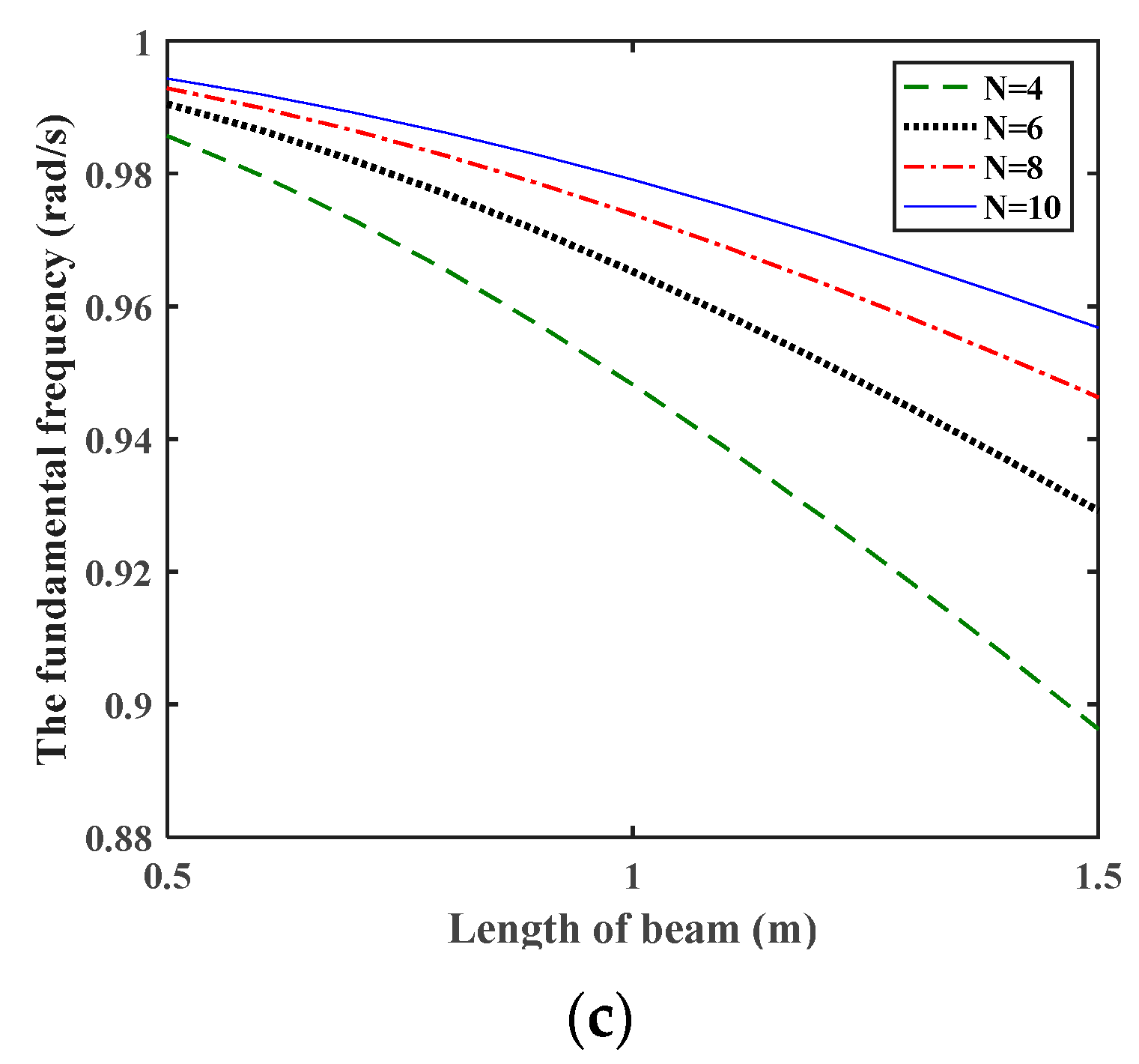
To verify the analysis results using FEM in the paper, a simulation is implemented, and the natural frequency feature is discussed below. For comparison, the flexible link is divided into a set of the different number of elements as $\left\{4,6,8,10\right\}$. The relationship of the fundamental frequency and three factors (i.e., angular velocity, payload mass, and length of the flexible link) with respect to the number of elements are illustrated in Figure 9. The first subfigure (a) shows the variation of the fundamental frequency with different angular velocity under the condition of payload mass as 1 kg and the beam length as 1 m. It is worth noting that the frequency becomes higher as the angular velocity increases. In other words, it also reflects the effect of the angular velocity on the stiffness of the flexible link. The next two subfigures (b) and (c) illustrate the effect of payload mass and length of flexible beam. It is evident that the frequency decreases with larger payload and longer beam length. Moreover, the iterative process costs more in computation time when the number of elements is larger than 10, while the corresponding results show no significant difference.

5. Conclusions

The paper focuses on the foreshortening effect of a rotating flexible link, which leads to the stiffening effect of the flexible link system. To study the rotating system in pick and place application, an SFF manipulator system including the effect of the flexible joint and the flexible link with tip payload is used as a research subject. The dynamic modeling is developed to analyze the features of natural frequency, which contributes to the model-based control of the SFF system.

The Hamilton principle is applied to deduce the governing equations of motion, considering the stiffening effect as the potential energy. Under the assumption of the small deformation of each point in free vibration, the motion equation is simplified, and the feature matrix is obtained to determine the natural frequencies of the SFF system. The results are compared with those in the literature. The method presented in this paper is more precise since the lower frequency is identified. Moreover, the modal shapes corresponding to each natural frequency are illustrated in detail.

Based on the constant rotational motion, it is concluded that the stiffening effect highly depends on the angular velocity. The stiffening effect of the flexible link becomes more prominent as a higher rotational velocity is adopted. Furthermore, the dynamic model of the SFF system, considering the stiffening effect, is studied using the finite element method with Hermite interpolation. The fundamental natural frequency results validate the conclusion that the system becomes stiffer when the foreshortening effect is considered in the modeling. Finally, the effect of three factors (i.e., angular velocity, mass of the payload, and length of the link) on the frequency are discussed respectively. The constant rotational velocity constraint used in the modeling will be dismissed to discuss the corresponding features in the next study. Moreover, the geometrically-exact beam theory will be employed to study the stiffening effect of the flexible link system in the future.