Abstract
This study explores the use of a photoionization detector (PID) to distinguish varieties of rosemary plant, based on their volatile organic compound (VOC) emissions. The aim was to be able to distinguish plant varieties using a simple, quick, and inexpensive method. Two varieties were studied, Rosmarinus officinalis L. “Prostratus” and “Erectus”. First, the PID was used to detect VOCs emitted by leaves from each variety, and subsequently essential oil was extracted from the same leaves. Then, the well-established GC-MS method was used to characterize and differentiate the oil from each of the two varieties. The PID was able to capture different signals, and a ‘fingerprint’ for each of the two varieties was obtained. To validate the PID performance, the data set obtained was analyzed by means of advanced statistical models (principal component analysis, cluster and support vector machine and artificial neural network) which were able to discriminate the two varieties with high accuracy (over 80%). Therefore, the results confirm that the PID was able to detect differences in VOC emissions. In conclusion, PID proved be an interesting instrument for the classification of rosemary plants, and in this sense could be applied to other aromatic plants.
1. Introduction
Aromatic plants are characterized by a particular aroma. This is the result of the production of an amazing diversity of volatile organic compounds (VOCs) by specialized secretory cells that are present in specific structures in these plants, called glandular trichomes [1,2]. VOCs are characterized by low molecular mass (between 50 and 200 Da), a low boiling point and high vapor pressure. A consequence of their high volatility is a marked tendency to pass from a liquid state to a vapor state, which allows them to disperse into the biosphere and act over long distances [2].
Plants that produce VOCs, in particular aromatic plants, have become an important economic resource worldwide. Among these plants, rosemary is widely cultivated, mainly due to its essential oil, which has high commercial value [3]. Rosemary leaf essential oil is dominated by monoterpenes (>90%), hydrocarbons and oxygenated compounds. Among rosemary species, several chemotypes can be distinguished, based on the predominant constituents of the essential oil. Examples include: 1,8-cineole; 1,8-cineole/α-pinene/camphor; myrcene; α-pinene/verbenone/bornyl acetate; and 1,8-cineole/borneol/p-cymene [4,5].
Sharma et al. (2020) [6] showed important variation in volatile components in R. officinalis var. albiflorus, with higher α-pinene (37.5%), 1,8-cineole (15.69%), verbenone (6.61%) and camphene (4.64%) compared to R. officinalis var. Gorizia, which yielded elevated 1,8-cineole (23.39%), α-pinene (13.14%), camphor (13.02%) and camphene (6.54%).
Furthermore, over 20 different types, varieties or cultivars can be distinguished as a function of morphological descriptors [4], such as the calyx, corolla, inflorescence and the presence of glandular trichomes [7], along with whether the plant is prostrate, its leaf size and flower characteristics [8,9].
Given this diversity, the ability to easily discriminate between the great variety of rosemary plants would be a step forward, in order to process specific, high-quality products. Thus, in the following, we develop a simple method to measure VOCs from rosemary leaves, in order to classify these aromatic plants.
The main analytical method used to measure VOCs is gas chromatography-mass spectrometry (GC–MS). It is widely used because of its high sensitivity, accuracy, reproducibility and overall robustness. However, disadvantages include the cost of equipment, the complexity of the operation and the long analysis time [10]. Depending on the aim of the analysis, a possible alternative is the use of a standalone photoionization detector (PID). These sensors are simple to use, inexpensive and the analysis only takes a few seconds. However, in turn, they also have some disadvantages. For example, a PID sensor can only measure a VOC concentration, and no information is provided about the chemical composition. In general, PID technology is designed to characterize the overall profile of a VOC mixture into a digital fingerprint, rather than quantify individual compounds [11].
However, the growing need for a rapid method to analyse VOC concentrations has stimulated interest in more wieldy instruments in terms of time, use and cost. The current literature contains reports from many studies that test the use of rapid VOC measurement instruments, in particular electronic noses [12].
To the best of our knowledge, no studies have investigated the use of a standalone PID to classify plants based on their VOC emissions. Unlike electronic noses, which use a pattern recognition algorithm to analyse several signals from an array of semi-selective gas sensors, we adopt a different approach. Specifically, we explore the response of a single PID to a wide range of VOCs, and the use of temporal data acquisition. The underlying idea in our approach is that signal kinetics in the time domain may be a function of the morphological (shape, dimension, histological classification) and physiological (essential oil composition) characteristics of rosemary plants. Our hypothesis is that the temporal kinetics of VOC emissions (emanation) from rosemary leaves have the potential to be a fingerprint for specific varieties. From this, it follows that the emission pattern could be used for classification purposes.
Therefore, two varieties of rosemary plants were studied. In a first step, PID technique was used to measure VOCs from the two varieties. Then, essential oils were extracted from each of the two varieties and characterized by GC-MS. The purpose of this step was to establish a baseline for differences between the varieties under examination. The analysis focused on whether the PID method would provide the same results as the GC-MS approach. PID data were analyzed using advanced statistical models to assess and verify the sensor’s classification capacity.
2. Materials and Methods
2.1. Materials
Two varieties of rosemary (Rosmarinus officinalis L. “Prostratus” and “Erectus”) were bought at a local plant nursery in Florence, Italy (Società Cooperativa Agricola di Legnaia). Only fresh leaves were used, and the mean moisture content was 76.3%.
Essential oil was extracted using petroleum ether (BAKER ANALYZED™ A.C.S. Reagent, J. T. Baker™, Houston, TX, USA). Samples were centrifuged and filtered to remove impurities, and stored at 4 °C until analysis.
A photoionization detector (PID) (PID-AH2, Alphasense Ltd., Great Notley, Braintree, UK) was used to determine the range of VOCs in the headspace over fresh rosemary leaves. The sensor was equipped with a 10.6 eV krypton lamp, and was sensitive to all target gases with photoionization potential less than or equal to this ionization threshold. The main features of the sensor, when used with isobutylene as the calibration gas, are as follows: minimum detection level 1 ppb; linear range (3% deviation) 40 ppm; overrange 40 ppm; sensitivity within the linear range >25 mV/ppm; full stabilization time (minutes to 20 ppb) 5; warm up time (time to full operation) 5 s; offset voltage 46–60 mV; and response time in diffusion mode <3 s. The main technical features are: power consumption 85 mW at 3.2 V (transient <300 mW for 200 ms); supply voltage 3.2–3.6 V DC; output signal as voltage ranging from the offset (minimum 46 mV) to the supply voltage minus 0.150 V.
The sensor was driven by a dedicated electronic interface (LabQuest2, Vernier, Beaverton, OR, USA), which supplied it with 3.6 V of DC power and contextually recorded the output DC voltage signal at a set acquisition frequency of 1 Hz (one reading per second). Output voltage signals were acquired as a function of time during each set of measurements, and stored locally by the software. Finally, all data were transferred to a computer and processed with Excel (Office 365, version 18.2008.12711.0).
2.2. Methods
Each plant was defoliated, and the leaves were homogenized to reduce internal variability. A total of 18 plants were studied, nine for each variety. Three replicates were conducted per day, alternating the two varieties each day, over a total of six days.
Essential oils were extracted from each plant. First, 5 g of fresh leaves was extracted using 45 mL of petroleum ether (BAKER ANALYZED™ A.C.S. Reagent, J. T. Baker™). For each sample, three washes were applied using 15 mL of solvent. Samples were then agitated using a vortex laboratory shaker. The extracted oils were centrifuged and filtered to remove impurities, and stored in dark glass bottles at 4 °C until analysis.
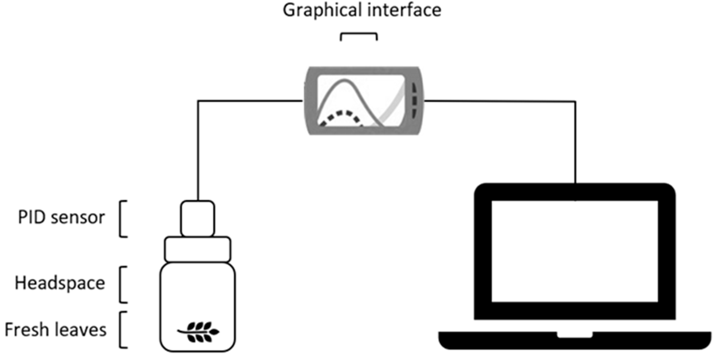
A bespoke measuring system was fitted to the PID sensor. The system consisted of a cylindrical thermostated (20 ± 1 °C) reading chamber with a nominal volume of 100 mL, made from polypropylene (Sarstedt, Numbrecht, Germany). The chamber was closed with a perforated screw cap, to allow a close connection with the sensor. Once the cap was screwed onto the chamber, the sensing side of the sensor was exposed to the air volume under measurement. The sensor was used in diffusion mode, above about 1 g of leaves. Before each measurement, it was ventilated for 5 min with ambient air using a laboratory fan at about 1600 L min−1, which established a steady baseline (it has humidity sensitivity that is near to 0). Then, the tested leaves were introduced into the measuring chamber and readings were recorded for 900 s (long enough for the sensor response to become stable). At the end of each measurement, the sensor–cap assembly was unscrewed from the measuring chamber and reventilated before the next measurement. Figure 1 shows the experimental setup.
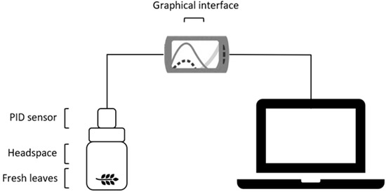
Figure 1.
VOC measurement using PID sensor technology.
2.3. GC-MS Analysis
The GC-MS analysis was conducted using the Agilent 7820 gas chromatograph coupled with a 5975C mass selective detector (Agilent Tech., Palo Alto, CA, USA). One microliter of extract in solution was injected into a split/splitless injector operating in splitless mode. A Gerstel MPS2 XL liquid autosampler was used. Chromatographic settings were as follows: injector in splitless mode set at 260 °C, J&W INNOWax column (30 m, 0.25 mm i.d., 0.5 µm df); oven temperature program: initial temperature 40 °C for 1 min, then 5 °C min−1 to 200 °C, then 10 °C min−1 to 220 °C, then 30 °C min−1 to 260 °C, held for 3 min. The mass spectrometer operated at 70 eV in scan mode, in the m/z range 29–330, at 3 scans s−1. Compounds were quantified using a calibration curve that was constructed by injecting known concentrations of authentic standard into the GC-MS. Deconvoluted peak spectra (obtained using the Agilent MassHunter software suite) were matched against the NIST 11 spectral library for initial identification. Kovats retention indices were calculated for further confirmation, and compared with those reported in the literature for the chromatographic column used.
2.4. Statistical Analysis
A one-way analysis of variance (ANOVA) was performed for the data collected by GC-MS, in order to characterize qualitative aspects of the essential oils obtained from the two varieties. A conventional F-test tested for significant main effects (p ≤ 0.05). The ANOVA was performed using R software (version 3.6.0 for Windows).
Data (voltage versus time) collected by the PID were transferred to a computer. Each sample was tested in triplicate, and the resulting data were normalized as a function of the mass of leaves in the measuring chamber in each run. Therefore, signal responses were averaged over the three replicates (runs) corresponding to each read time. Then, for the purposes of drift compensation, the PID’s base reading was removed. Specifically, at each read time, the voltage baseline was subtracted from the recorded response.
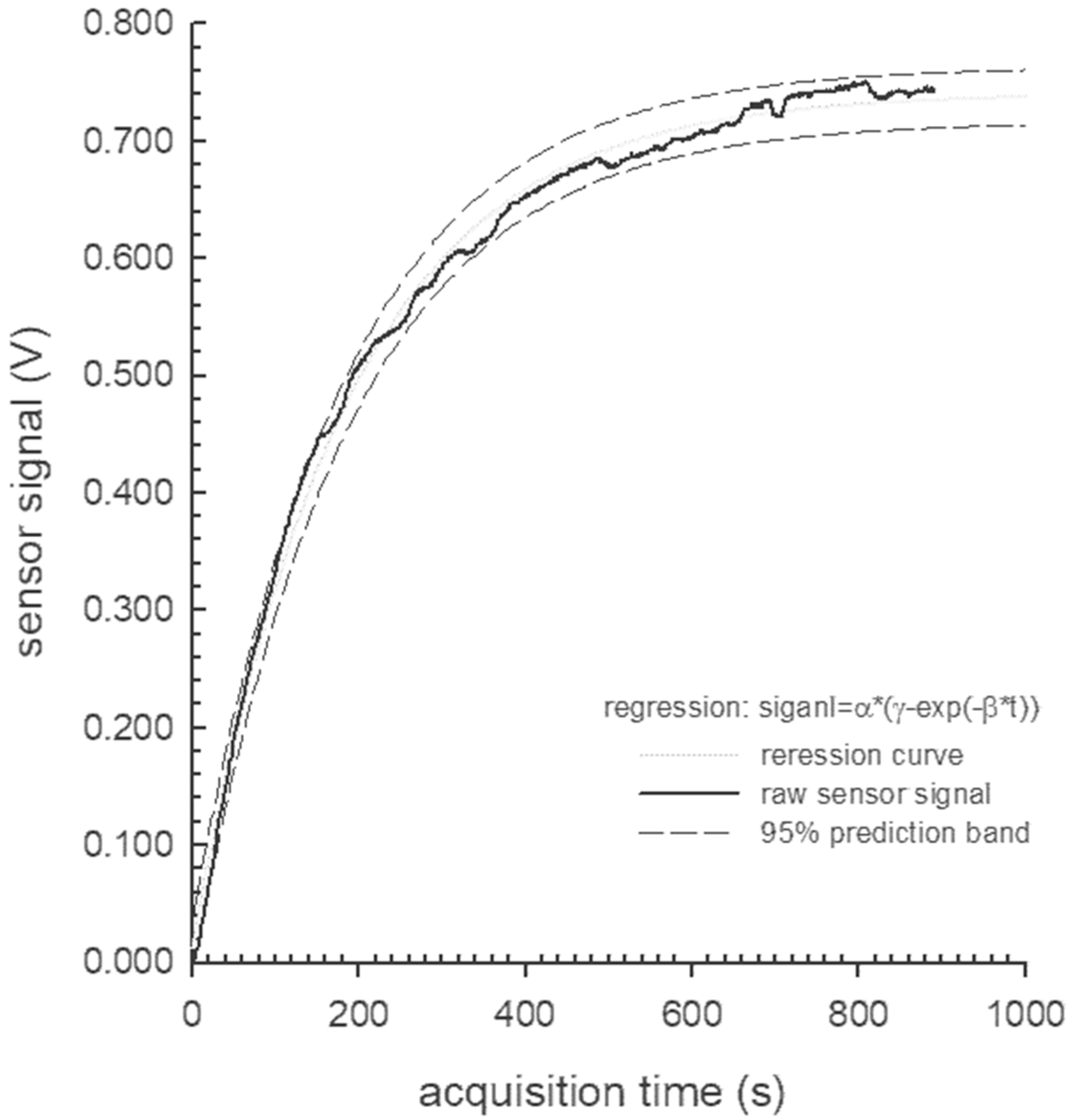
Then, the signal was regressed over time, in order to identify the best non-linear model fit for the data. This was conducted for each data series using CurveExpert 1.40 software (D. Hyams, 1995–2009, Microsoft Corporation). The latter is a regression/ fitting tool that uses the Levenberg–Marquardt method to solve nonlinear regressions, making it possible to rank best-fit models on the basis of the coefficient of determination. All the tested data series proved to be well-fitted by a three-parameter exponential model, with r2 ranging from 0.95 to 0.99:
where α, β, and γ are the model parameters, and t is the acquisition time.
This model was then reapplied to each replicated data series and rechecked for goodness of fit using SigmaPlot 10.0 software (Systat Software Inc., San Jose, CA, USA). This software package adopts an iterative approach that is based on the Levenberg–Marquardt algorithm, and aims to minimize the sum of the squared differences between observed and predicted values of the dependent variable during regression testing. An example of the output of this analysis is reported in Table 1.

Table 1.
Statistical output of the nonlinear regression (dynamic fitting).
In addition to the exponential model, four other parameters were used to describe the signal versus time kinetic: (i) the grand mean (GM) and (ii) the corresponding standard deviation (GMsd), both computed over the entire reading time (1–900 s); (iii) the maximum recorded value (Max); and (iv) the area under the curve (AUC). The latter was calculated following a numerical quadrature approach, as the definite integral of signal values between 1 and 1800 s read time.
Following the application of this procedure, seven features of the sensor signal were identified and used in the subsequent multivariate pattern recognition techniques:
- -
- α, β, and γ (the exponential model parameters)
- -
- GM (the grand mean of readings computed over a data series acquisition time)
- -
- GMsd (standard deviation of readings computed over a data series acquisition time)
- -
- Max (the maximum signal reading)
- -
- AUC (the area under the curve).
The complex set of data collected by the PID technique were then interpreted with several statistical models: principal component analysis (PCA), support vector machine (SVM), cluster analysis (CA), and artificial neural networks (ANN).
PCA is the most widely used pattern recognition method applied to sensor data [13]. This linear, unsupervised technique is used to analyse, classify and reduce the dimensionality of numerical datasets in a multivariate problem [14]. PCA was performed using the XLSTAT Premium software package.
CA is an exploratory multivariate technique that is used to explore the dataset. It tries to identify natural groupings among data points, and presents these groups in the form of a dendrogram or hierarchical tree [15]. It is based on the determination of the distance between objects (degree of similarity/ dissimilarity), and the application of an agglomerative (amalgamation) method to establish clusters of n-objects. The CA was performed using R software (version 3.6.0 for Windows).
The SVM technique is one of the most widely applied classification methods in electronic nose technologies. It was developed for the linear classification of separable data, but can be applied to nonlinear data with the use of kernel functions. The principal idea is that separating classes by a particular hyperplane maximizes a quantity called the margin. The margin corresponds the distance from the closest point in the dataset to a hyperplane dividing the classes [16]. Four kernel types are available: linear, polynomial, radial basis function and sigmoid. Different kernel functions were tested to check the robustness of the classifier model [16]. The SVM analysis was performed using XLSTAT Premium software.
The ANNs are programs conformed on the networks of the central nervous system (neural). These networks are compounded interconnection nodes (neurons) able of identify patterns and relationships in data [17]. ANN is made up of many artificial neurons, organized in layers, which form a network. An artificial neuron is a simple processing element that, as with biological neurons, receives signals from different inputs to produce an output [18]. JustNN software (version 4.0) was used for the analysis. JustNN is a free software package; it is easy to use, frequently updated, and performs well. The model is based on three layers of nodes: input, hidden and output. Based on the inputs in the first layer, and the outputs from the third layer, the model develops a number of hidden nodes that comprise the middle layer [19].
3. Results
Our results can be divided into three broad areas. The first was the GC-MS characterization of essential oils. Here, the aim was to differentiate between the two varieties of plants and establish a baseline for the rest of the study. Then, a generic PID was used to detect VOCs from the same batches of fresh leaves, in order to try to classify the two varieties based on their emissions. Finally, the two sets of measurements were compared. The complex dataset was processed with advanced statistical models (PCA, CA, SVM and ANN) to validate PID measurements.
3.1. Essential Oil Characterization
A total of 26 components, accounting for >95% of the essential oils, were identified. Table 2 reports the percentages of the main compounds (≥1%) found in the two essential oils. This highlights that “Erectus” is characterized by a high level (30.40 ± 1.71%) of bornyl acetate followed by alpha-pinene (13.17 ± 0.85%). “Prostratus” is characterized by alpha-pinene (35.30 ± 1.50%) followed by bornyl acetate (13.31 ± 0.62%). Thus, alpha-pinene and bornyl acetate are the compounds with the highest differences between the two varieties. They are followed by camphor (8.28 ± 0.42% and 8.10 ± 0.35%), and camphene (8.07 ± 0.30% and 10.02 ± 0.70%) for “Prostratus” and “Erectus”, respectively.
Table 2.
Chemical composition of essential oils (≥1%) for the two rosemary varieties (mean ± standard deviation) (n = 3). Letters (a, b) indicate statistically significant differences using the Tukey HSD post hoc test (p < 0.05).
3.2. PID Measurements
Goodness of fit, representative of all of the analyzed data series, is reported in Table 2 (see Figure 2 for a graphical representation). Table 2 shows that the model converges after 87% of iterations, with an adjusted R2 of 0.9956 and a standard error of estimate of 0.0119. All three parameters describing the model were significantly different from zero at p ≤ 0.001, and the ANOVA of the regression proved to be significant at the same level. As stated earlier, these results were representative of all of the tested data series; thus, the chosen model fits the PID data.

Figure 2.
Statistical goodness of fit model.
3.3. Data Analysis
3.3.1. Principal Component Analysis
A PCA was run on the dataset. The first two components (F1, F2) explained nearly 82.59% of total variance, accounting for 60.59 and 22.00%, respectively. The scatter plot shown in Figure 3 reports the projection of variables on F1 and F2 axes. Here, the aim was to determine which variables influenced the distinction between the two varieties. A visual inspection shows the “Erectus” variety in the right quadrant, and “Prostratus” in the left; hence the two varieties can be clearly distinguished. Figure 3 highlights that the variables that have the greatest influence on the distinction between the two varieties are MAX, AUC, GM and GMsd (for F1), and α, β, and γ (for F2).
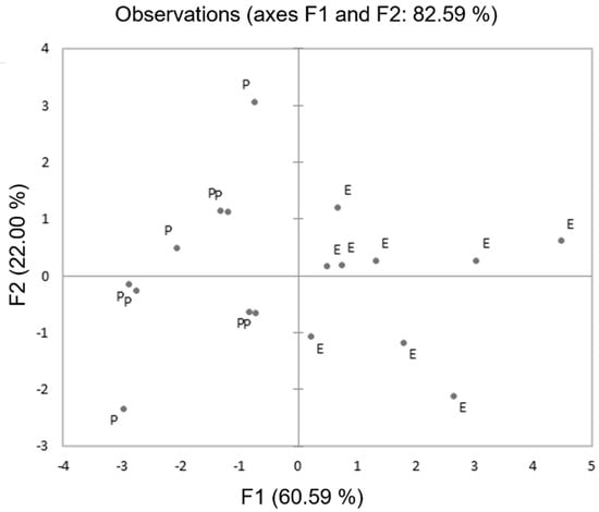
Figure 3.
Biplot of the PCA of the two rosemary varieties. P—“Prostatus”, E—“Erectus”.
3.3.2. Cluster Analysis
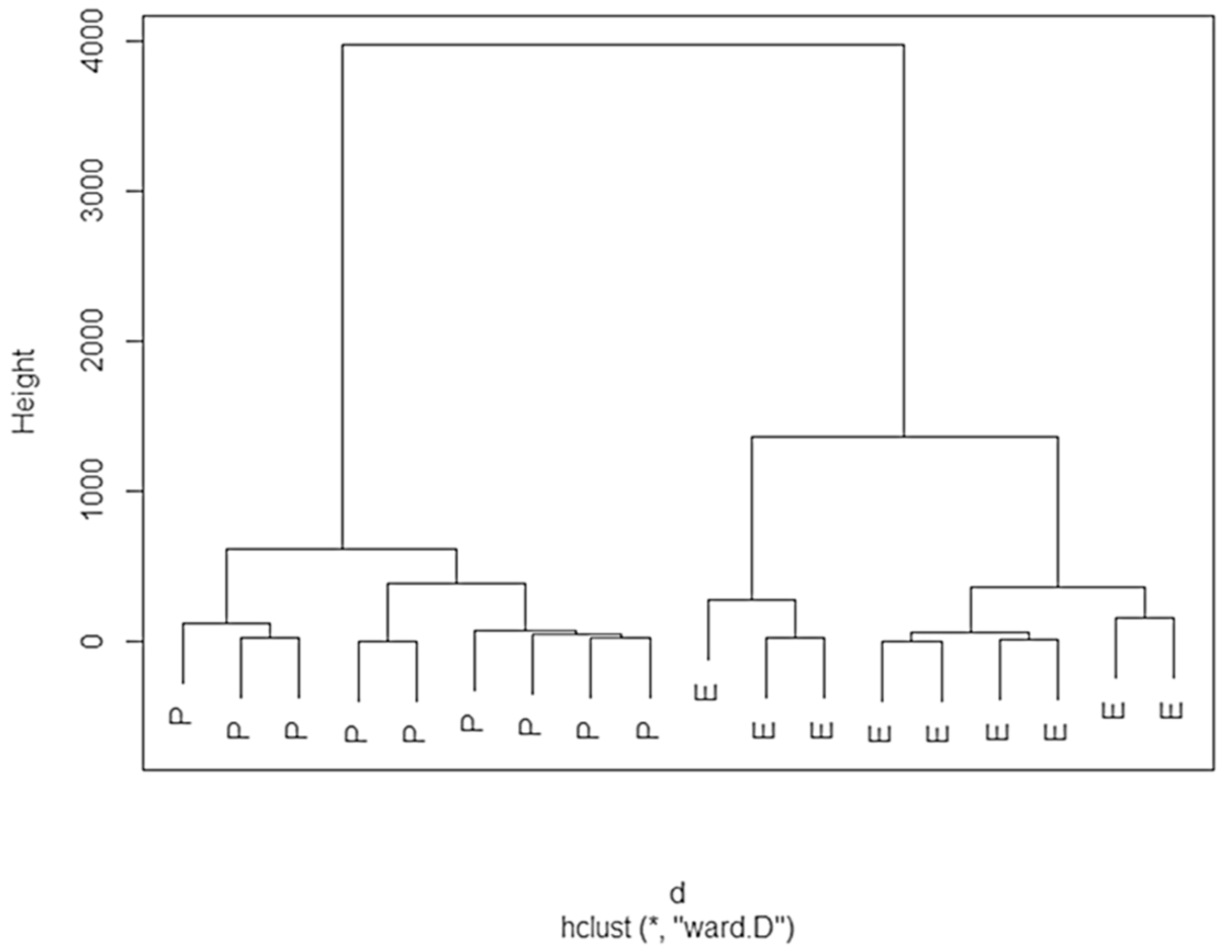
A hierarchical CA was run on the dataset, using the squared Euclidean distance as a measure of similarity and Ward’s method as the amalgamation rule. The dendrogram is reported in Figure 4. This analysis subdivided the two rosemary varieties into two large groups. The first subgroup contains “Prostratus” plants, and the other contains “Erectus” plants. Thus, the two varieties were clearly classified by CA.
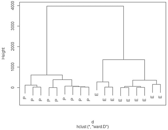
Figure 4.
Dendrogram obtained by a cluster analysis of the two rosemary varieties. P—“Prostatus”, E—“Erectus”.
3.4. Support Vector Machine
The SVM technique was used to discriminate between rosemary varieties based on PID sensor data. Different kernel functions were tested to check the robustness of the classifier model, and a linear kernel was chosen. Cross-validation was applied to all data in the six test cycles. Classification was good, and the accuracies of the training and validation samples were found to be 100 and 83.33%, respectively. The results are reported in Table 3 and Table 4.
Table 3.
Confusion matrix for the training sample (VAR–E/P).
Table 4.
Confusion matrix for the validation sample (VAR–E/P).
3.5. Artificial Neural Networks
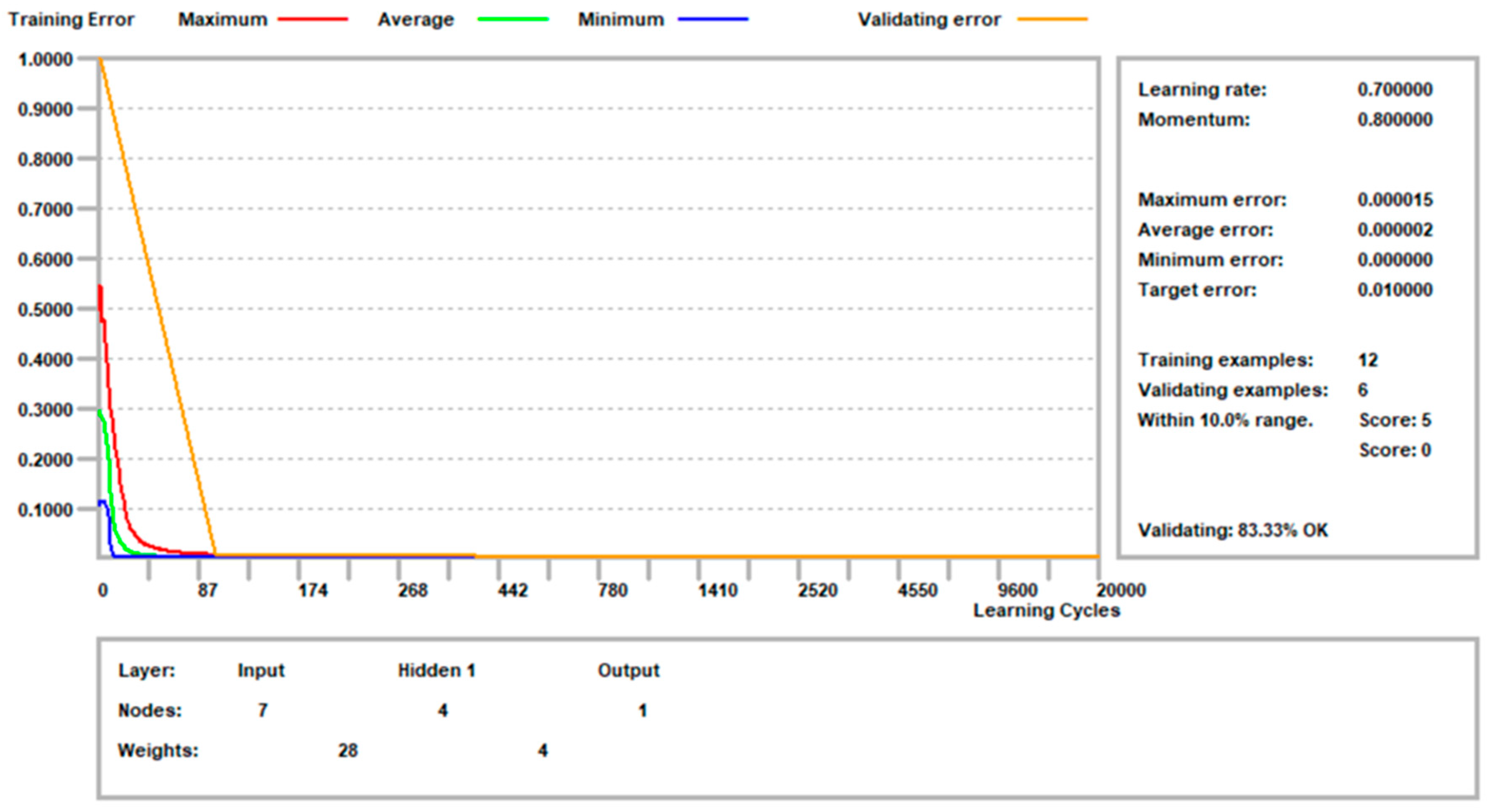
The software was trained using the backpropagation error algorithm with the following settings: learning rate 0.7; momentum 0.80. The target error was fixed when the average error was 0.01. One hundred cycles were run before the validation cycle, and 100 validation cycles were run. The learning process ended when all of the validation samples were within 10% of the validation error. The results are shown in Figure 5.
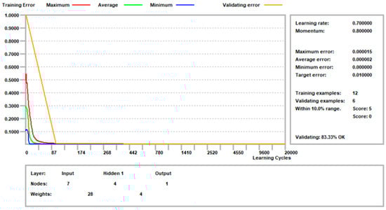
Figure 5.
The ANN learning process.
The analysis was run with 12 training samples, and six samples were randomly chosen for validation. The process ended after 2000 cycles, with an average error rate of 0.000002. Validation accuracy was 83.33%.
Figure 6 is a graphic visualization of the neural network in justNN.
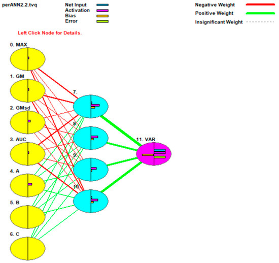
Figure 6.
Graphic visualization of the neural network in ANN.
In Figure 6, the yellow circles represent the seven inputs: Max, GM, GMsd, AUC and A, B, C (corresponding to α, β, and γ, respectively). The light blue circles are hidden nodes, and the purple node is the output, the rosemary variety. Lines between nodes represent relations between levels. The thickness of the line highlights the importance of the relation between variables. The thicker the line, the stronger the relationship. Red and green lines represent negative and positive relationships between inputs and outputs, respectively.
Finally, the absolute and relative importance of each input column is reported in Figure 7. Importance is the sum of the absolute weights of connections from input nodes to all of the nodes in the first hidden layer. Inputs are shown in descending order of importance.
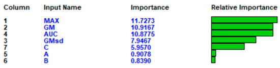
Figure 7.
ANN learning cycle parameters.
4. Discussion
In this study, a PID detector was used to discriminate between two varieties of rosemary plants based on VOCs emission. To our knowledge, this is the first study on the use of a PID used for the particular purpose of discriminating different varieties in the field of aromatic plants. PID is one of the most popular techniques on the market for the detection of VOCs in the ppb range [20].
Our approach was to use a PID detector as a quick, easy, and relatively inexpensive method for the classification of different varieties of rosemary plants.
In the current literature, some studies have addressed the same topic using more complex technologies. Khorramifar et al. [21] reported a rapid discrimination between grape cultivars (Vitis vinifera L.) using e-nose technology with a high detection accuracy using five chemometric methods, including PCA, LDA, QDA, SVM, and ANN. In other study [22], different potato cultivars have been studied using e-nose technology with regard to VOC emission. Again, the results showed high detection accuracy and the cultivars were precisely identified. Similar results have been obtained by Abbas Gorji-Chakespari et al. [23] concerning the classification of essential oils in Rosa damascena Mill. using an e-nose.
In our study, the strategy was simpler and a single PID detector was used. The idea was that signal kinetics in the time domain might be a function of the morphological (shape, dimension, histological classification) and physiological (essential oil composition) characteristics of rosemary plants. Our hypothesis was that the temporal kinetics of VOC emissions (emanation) from rosemary leaves have the potential to be a fingerprint for specific varieties.
Therefore, the first result of this study was to ensure that the PID was capable of measuring VOC emissions from rosemary leaves, and encouraging results were obtained. The data collected from the VOC emission readings of the two rosemary varieties were analyzed and well-fitted by an exponential model described by three parameters with a corrected R2 of 0.9956 and a standard error of estimate of 0.0119.
All three parameters describing the model were significantly different from zero at p ≤ 0.001 and the ANOVA of the regression was significant at the same level. This could be an important achievement in light of the current trend to seek innovative solutions for VOC monitoring and detection based on the use of small, portable instruments that are immediate and easy to read [24].
The ANOVA identified a significant main effect with respect to qualitative aspects of the two varieties of rosemary plants. In general, significant differences were seen between the two varieties for all of the reported compounds. Both the identified compounds and their percentages are consistent with the results reported in the current literature [25,26]. The results obtained allowed us to state that the two varieties used for the study did indeed have two different varietal profiles.
Thus, the second encouraging result was that different signals were recorded for the two varieties. This demonstrated that it was possible to obtain a sort of “fingerprint” for each variety studied. As the two varieties were correctly identified, this confirmed that the PID can be used for classification purposes, which was the main aim of the present study.
Furthermore, data analyses using different statistical models were satisfactory. Here, the aim was to interpret the dataset recorded by the PID. The two unsupervised methods (PCA and CA) were able to distinguish the two varieties. The PCA accurately differentiated the two varieties: 82.59% of total variance was explained by F1 and F2 (60.59% and 22.00%, respectively). The variables that were most influential in distinguishing the two varieties were MAX, GM, AUC and GMsd (for F1), and α, β, and γ, (for F2). The same result was achieved by CA. Here, two homogeneous groups were obtained: “Erectus” and “Prostatus” varieties. Our results agree with the current literature [21,23].
Similar results were obtained using supervised methods. The ANN found a classification validation rate of 83%. Here, the variables that most influenced training were MAX, AUC, GM, GMsd, α, β, and γ, in descending order of importance. A good classification rate was also obtained with SVM analysis, where validation accuracy was found to be 83.33%.
Hence, the two rosemary varieties were clearly separated by all the models with a high degree of accuracy and these findings verify the usefulness of the PID as a classification tool.
A limitation of the PID sensor application could be that it does not provide any information on the chemical composition of VOCs, and rather only measures their concentration. However, the aim of this study was to characterize the profile of rosemary plant varieties based on the VOC mixture emitted as a digital fingerprint, rather than to quantify individual components. The encouraging results obtained from this first study could be a starting point for the development of PID technology as a discrimination method in this field of application.
5. Conclusions
This study investigated whether a general-purpose, cheap, and easy-to-use PID could distinguish between two varieties of rosemary plant. The device was able to record two different VOC emission base signals, and provided a ‘fingerprint’ for each variety. Advanced statistical models (PCA, CA, SVM and ANN) were applied to validate PID performance. Each model demonstrated high classification accuracy (>80%). Both supervised and unsupervised methods were able to clearly distinguish the two varieties. Although there is clearly scope to improve the device, both in terms of performance and design, this study shows that it already functions very well, and further studies could focus on optimization.
Author Contributions
Conceptualization, A.S., G.A. and P.M.; methodology, P.M. and A.S.; software, A.S. and F.M.; validation, A.S. and G.A.; formal analysis, A.S., L.C., F.C. and F.M.; investigation, A.S. and L.G.; resources, P.M. and A.P.; data curation, A.S., G.A. and P.M.; writing—original draft preparation, A.S.; writing—review and editing, A.S., G.A., F.C. and P.M.; visualization, P.M.; supervision, P.M. and A.P. All authors have read and agreed to the published version of the manuscript.
Funding
This research received no external funding.
Institutional Review Board Statement
Not applicable.
Informed Consent Statement
Not applicable.
Data Availability Statement
Not present.
Conflicts of Interest
The authors declare no conflict of interest.
References
- Werker, E. Trichome Diversity and Development Department of Botany, The Hebrew University of Jerusalem. Adv. Bot. Res. 2000, 31, 1–35. [Google Scholar]
- Wheatley, R.E. The Consequences of Volatile Organic Compound Mediated Bacterial and Fungal Interactions. Antonie Van Leeuwenhoek 2002, 81, 357–364. [Google Scholar] [CrossRef] [PubMed]
- Borges, R.S.; Ortiz, B.L.S.; Pereira, A.C.M.; Keita, H.; Carvalho, J.C.T. Rosmarinus Officinalis Essential Oil: A Review of Its Phytochemistry, Anti-Inflammatory Activity, and Mechanisms of Action Involved. J. Ethnopharmacol. 2019, 229, 29–45. [Google Scholar] [CrossRef]
- Ribeiro-Santos, R.; Carvalho-Costa, D.; Cavaleiro, C.; Costa, H.S.; Albuquerque, T.G.; Castilho, M.C.; Ramos, F.; Melo, N.R.; Sanches-Silva, A. A Novel Insight on an Ancient Aromatic Plant: The Rosemary (Rosmarinus Officinalis L.). Trends Food Sci. Technol. 2015, 45, 355–368. [Google Scholar] [CrossRef]
- Boutekedjiret, C.; Bentahar, F.; Belabbes, R.; Bessiere, J.M. The Essential Oil from Rosmarinus Officinalis L. in Algeria. J. Essent. Oil Res. 1998, 10, 680–682. [Google Scholar] [CrossRef]
- Sharma, Y.; Schaefer, J.; Streicher, C.; Stimson, J.; Fagan, J. Qualitative Analysis of Essential Oil from French and Italian Varieties of Rosemary (Rosmarinus Officinalis L.) Grown in the Midwestern United States. Anal. Chem. Lett. 2020, 10, 104–112. [Google Scholar] [CrossRef]
- Zaouali, Y.; Bouzaine, T.; Boussaid, M. Essential Oils Composition in Two Rosmarinus Officinalis L. Varieties and Incidence for Antimicrobial and Antioxidant Activities. Food Chem. Toxicol. 2010, 48, 3144–3152. [Google Scholar] [CrossRef]
- Fadel, O.; El Kirat, K.; Morandat, S. The Natural Antioxidant Rosmarinic Acid Spontaneously Penetrates Membranes to Inhibit Lipid Peroxidation in Situ. Biochim. Biophys. Acta Biomembr. 2011, 1808, 2973–2980. [Google Scholar] [CrossRef] [Green Version]
- Benbelaïd, F.; Khadir, A.; Bendahou, M.; Zenati, F.; Bellahsene, C.; Muselli, A.; Costa, J. Antimicrobial Activity of Rosmarinus Eriocalyx Essential Oil and Polyphenols: An Endemic Medicinal Plant from Algeria. J. Coast. Life Med. 2016, 4, 39–44. [Google Scholar] [CrossRef]
- Agbroko, S.O.; Covington, J. A Novel, Low-Cost, Portable PID Sensor for the Detection of Volatile Organic Compounds. Sens. Actuators B Chem. 2018, 275, 10–15. [Google Scholar] [CrossRef] [Green Version]
- Laothawornkitkul, J.; Moore, J.P.; Taylor, J.E.; Possell, M.; Gibson, T.D.; Hewitt, C.N.; Paul, N.D. Discrimination of Plant Volatile Signatures by an Electronic Nose: A Potential Technology for Plant Pest and Disease Monitoring. Environ. Sci. Technol. 2008, 42, 8433–8439. [Google Scholar] [CrossRef] [PubMed]
- Kiani, S.; Minaei, S.; Ghasemi-Varnamkhasti, M. Application of Electronic Nose Systems for Assessing Quality of Medicinal and Aromatic Plant Products: A Review. J. Appl. Res. Med. Aromat. Plants 2016, 3, 1–9. [Google Scholar] [CrossRef]
- Capone, S.; Epifani, M.; Quaranta, F.; Siciliano, P.; Taurino, A.; Vasanelli, L. Monitoring of Rancidity of Milk by Means of an Electronic Nose and a Dynamic PCA Analysis. Sens. Actuators B Chem. 2001, 78, 174–179. [Google Scholar] [CrossRef]
- Costache, G.N.; Corcoran, P.; Puslecki, P. Combining PCA-Based Datasets without Retraining of the Basis Vector Set. Pattern Recognit. Lett. 2009, 30, 1441–1447. [Google Scholar] [CrossRef]
- Zhou, B.; Wang, J. Discrimination of Different Types Damage of Rice Plants by Electronic Nose. Biosyst. Eng. 2011, 109, 250–257. [Google Scholar] [CrossRef]
- Sanaeifar, A.; Mohtasebi, S.S.; Ghasemi-Varnamkhasti, M.; Ahmadi, H.; Lozano, J. Development and Application of a New Low Cost Electronic Nose for the Ripeness Monitoring of Banana Using Computational Techniques (PCA, LDA, SIMCA, and SVM). Czech J. Food Sci. 2014, 32, 538–548. [Google Scholar] [CrossRef] [Green Version]
- Huang, R.S.P.; Nedelcu, E.; Bai, Y.; Wahed, A.; Klein, K.; Tint, H.; Gregoric, I.; Patel, M.; Kar, B.; Loyalka, P.; et al. Post-Operative Bleeding Risk Stratification in Cardiac Pulmonary Bypass Patients Using Artificial Neural Network. Ann. Clin. Lab. Sci. 2015, 45, 181–186. [Google Scholar]
- Lozano, J.; Santos, J.P.; Horrillo, M.C. Classification of White Wine Aromas with an Electronic Nose. Talanta 2005, 67, 610–616. [Google Scholar] [CrossRef]
- Mazzocchi, C.; Corsi, S.; Sali, G. Agricultural Land Consumption in Periurban Areas: A Methodological Approach for Risk Assessment Using Artificial Neural Networks and Spatial Correlation in Northern Italy. Appl. Spat. Anal. Policy 2017, 10, 3–20. [Google Scholar] [CrossRef]
- Xu, W.; Cai, Y.; Gao, S.; Hou, S.; Yang, Y.; Duan, Y.; Fu, Q.; Chen, F.; Wu, J. New Understanding of Miniaturized VOCs Monitoring Device: PID-Type Sensors Performance Evaluations in Ambient Air. Sens. Actuators B Chem. 2021, 330, 129285. [Google Scholar] [CrossRef]
- Khorramifar, A.; Karami, H.; Wilson, A.D.; Sayyah, A.H.A.; Shuba, A.; Lozano, J. Grape Cultivar Identification and Classification by Machine Olfaction Analysis of Leaf Volatiles. Chemosensors 2022, 10, 125. [Google Scholar] [CrossRef]
- Khorramifar, A.; Rasekh, M.; Karami, H.; Malaga-Toboła, U.; Gancarz, M. A Machine Learning Method for Classification and Identification of Potato Cultivars Based on the Reaction of MOS Type Sensor-Array. Sensors 2021, 21, 5836. [Google Scholar] [CrossRef] [PubMed]
- Gorji-Chakespari, A.; Nikbakht, A.M.; Sefidkon, F.; Ghasemi-Varnamkhasti, M.; Valero, E.L. Classification of Essential Oil Composition in Rosa Damascena Mill. Genotypes Using an Electronic Nose. J. Appl. Res. Med. Aromat. Plants 2017, 4, 27–34. [Google Scholar] [CrossRef]
- Tholl, D.; Hossain, O.; Weinhold, A.; Röse, U.S.R.; Wei, Q. Trends and Applications in Plant Volatile Sampling and Analysis. Plant J. 2021, 106, 314–325. [Google Scholar] [CrossRef]
- Li, G.; Cervelli, C.; Ruffoni, B.; Shachter, A.; Dudai, N. Volatile Diversity in Wild Populations of Rosemary (Rosmarinus Officinalis L.) from the Tyrrhenian Sea Vicinity Cultivated under Homogeneous Environmental Conditions. Ind. Crops Prod. 2016, 84, 381–390. [Google Scholar] [CrossRef]
- Carrubba, A.; Abbate, L.; Sarno, M.; Sunseri, F.; Mauceri, A.; Lupini, A.; Mercati, F. Characterization of Sicilian Rosemary (Rosmarinus Officinalis L.) Germplasm through a Multidisciplinary Approach. Planta 2020, 251, 37. [Google Scholar] [CrossRef]


Publisher’s Note: MDPI stays neutral with regard to jurisdictional claims in published maps and institutional affiliations. |
© 2022 by the authors. Licensee MDPI, Basel, Switzerland. This article is an open access article distributed under the terms and conditions of the Creative Commons Attribution (CC BY) license (https://creativecommons.org/licenses/by/4.0/).