Use of Surface Acoustic Waves for Crack Detection on Railway Track Components—Laboratory Tests

Abstract

The present work investigates the technical feasibility of a condition monitoring setup aiming at the detection of gauge corner cracks (aka head checks) in pearlitic railway rails, using a wayside (i.e., stationary) setup with surface acoustic waves (SAW) as its detection principle. The experimental SAW setup consists of a pitch-catch setup using piezo transducers equipped with comb adaptors to excite and measure narrowband Rayleigh waves with a center frequency of 1 MHz. SAW experiments were performed on a rail subjected to cyclic loading in a 1:1 wheel–rail test rig yielding the specific rolling contact fatigue, i.e., head checks. Elastodynamic finite integration technique (EFIT) simulations were performed to analyze the surface and bulk wave propagation in the rail and to predict the signals at specific receiver positions. SAW transmission and reflection scenarios at cracks were analyzed numerically via modelled variations of gauge corner crack configurations according to number of cracks (0–3) and depth (0, 0.5 mm and 1 mm). The numerical and the experimental results each show a clear correlation between the appearance and intensity of head check damage and the wave attenuation in transmission mode.

1. Introduction

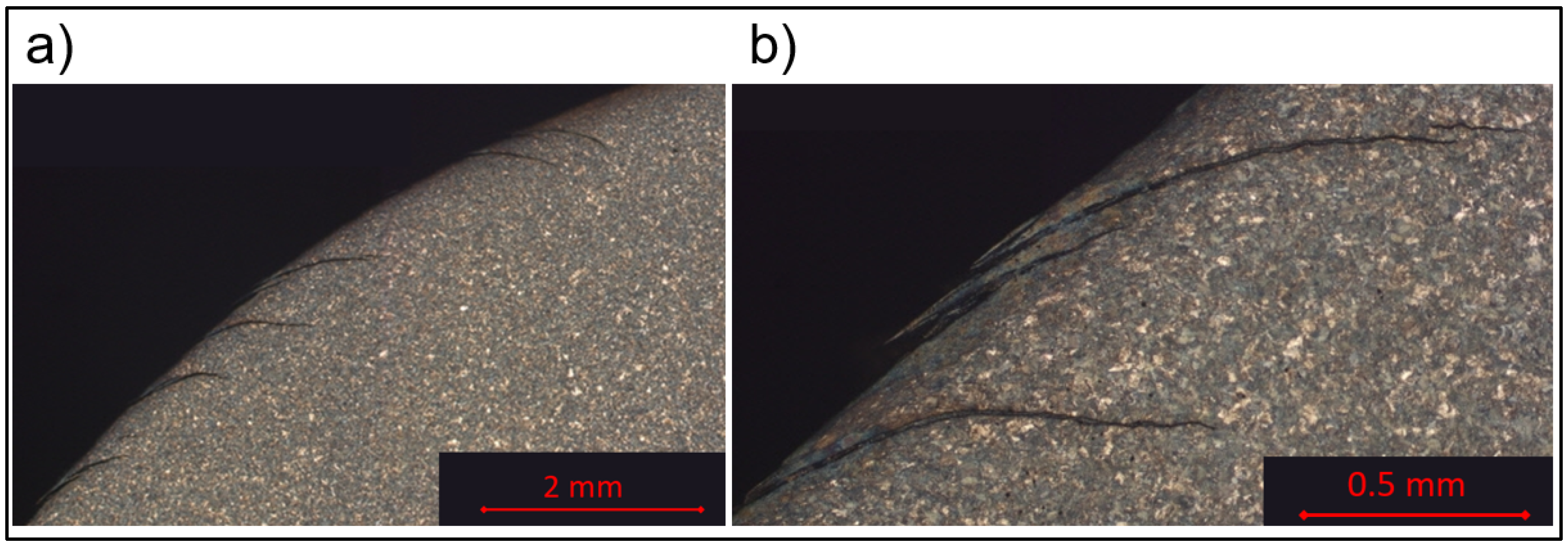
1.1. Head Checks—A Specific Type of Rail Damage

Near-surface defects arising from rolling contact fatigue (RCF) are a major source of concern in railway operations worldwide. Among the different damage types related to RCF, head checks have become the most prominent since they pose a high risk of complete rail failure and are a major driver of maintenance costs. Head checks form a closely spaced network of almost parallel-aligned cracks on the gauge corner on high rails at turns. These surface cracks initially grow at a shallow angle to the rail, posing a challenge for detection at an early stage. A description of head checks and how they can be generated in a laboratory setup, i.e., a 1:1 wheel rail test rig can be found in reference [1].

1.2. Current Technical Solutions for Condition Monitoring of Railway Tracks

Preventive maintenance strategies dictate regular maintenance activities to grind or mill the top surface layer of rails, to remove these cracks and ensure safe railway operation.

In order to schedule rail maintenance interventions effectively, it is vital to detect these surface defects as early as possible. Railway infrastructure providers generally have two complementing measurement options for measuring and monitoring the track condition: (a) measurements with instrumented trains that regularly scan the whole track network, and (b) stationary measurements currently limited to sensors placed at hotspots within the track network or on critical safety components such as switches and crossings. The latter is referred to as wayside condition monitoring. Currently available technical solutions for wayside monitoring of the track are limited to strain and load measurements to identify unbalanced and overloaded freight wagons, and vibration sensor instrumentation to identify defective wheels (e.g., flat spots). Driven by the need for condition-based maintenance (CBM) of rolling stock and track, extensions of these concepts are currently gaining increased interest [2].

1.3. Surface Acoustic Waves for Crack Detection

In this paper, the term surface acoustic wave (SAW) refers to ultrasonic waves that propagate along surfaces similarly to Rayleigh waves, with the difference that the propagation medium is not an elastic half-space but a body with geometrical dimensions much larger than the wavelength. These waves may also be termed quasi-Rayleigh waves. A promising method for permanent monitoring of components with regard to surface cracks is to employ surface acoustic waves for crack detection and characterization [3]. To this end, surface acoustic waves are excited at one point of the structure, and the transmitted waves are detected at another point. The detected signal changes if a crack grows between the excitation and the detection points, since the crack acts as an obstacle in the wave path [3,4]. Possible techniques for the excitation of surface acoustic waves are electromagnetic acoustic transducers (EMAT) [5], piezoelectric transducers equipped with wedge or comb adaptors [6], or pulsed laser beams [3]. Masurkar et al. recently published a paper dealing with the location of surface and sub-surface defects in rail tracks, using Rayleigh waves excited and measured via a non-contacting approach [7]. The main differences between their work and the work presented here will be discussed in the corresponding section on specimen and measurement setup. The goal of the present work is to investigate the feasibility of the SAW-based approach using mobile transducer equipment and wave propagation simulations, to pave the way for the design of a permanent installation.

2. Test Specimen and Methods

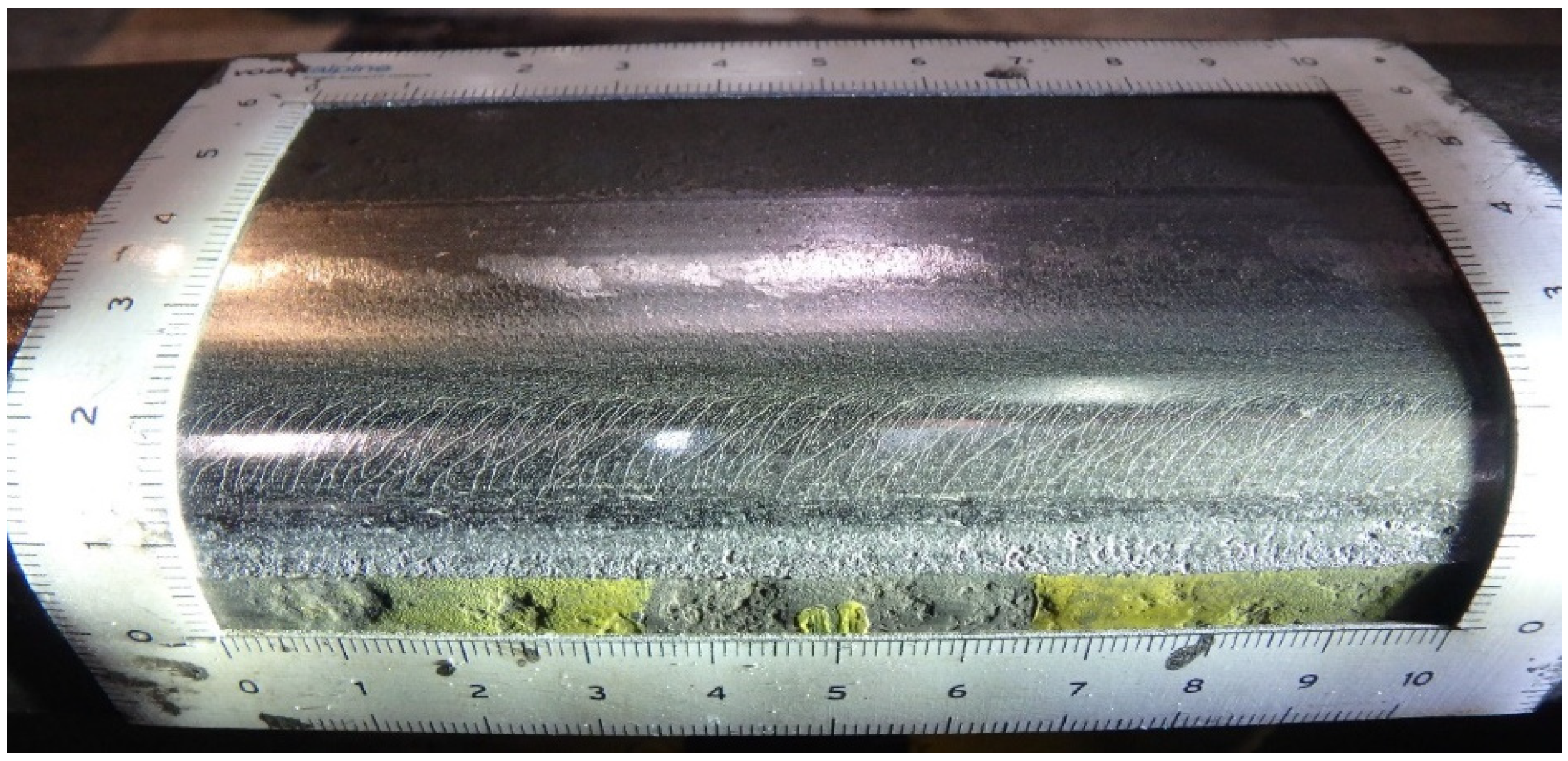
2.1. Generation of Head Checks in a 1:1 Wheel–Rail Test Setup

The evolution of gauge corner cracks (head checks) in rails is related to the wheel–rail contact that in turn depends on the geometries of the rail and the passing wheels as well as the local friction conditions. One aim of building a 1:1 wheel–rail laboratory setup was to identify the contact conditions that lead to this specific damage pattern observed in track. A more detailed description of the test rig, testing procedure and the evolution of head checks can be found in ref. [1,8]. To monitor the generation and growth of head checks, a 1.5 m long standard rail (material R260, rail profile 60E1 (UIC60)) was subjected to cyclic testing in the voestalpine wheel–rail test rig with friction–load parameters that are known to produce the targeted damage pattern “head checks” [1,8]. The corresponding RCF experiment took approximately 2 weeks; SAW measurements were performed during dedicated breaks, hence the following results exhibit unequal measurement intervals.

After approximately 15,000 load cycles (i.e., wheel passes), cracks had initiated in the rail; after ~25,000 cycles, a typical head check pattern started to evolve; and after 70,000 cycles the head check pattern clearly covered the full length of wheel–rail contact. Figure 1 shows an image of the head check pattern at the end of the experiment, i.e., after 310,000 wheel passes. Note that in contrast to the experiments performed by Masurkar et al. [7], where “the specimens were initially polished in order to remove any unwanted rust which would affect the propagation of Rayleigh wave”, the aim of the present study was to investigate rails with a typical RCF damage pattern and close to service conditions; therefore, the rail was deliberately left unpolished, retaining any existing rust or wear particles.

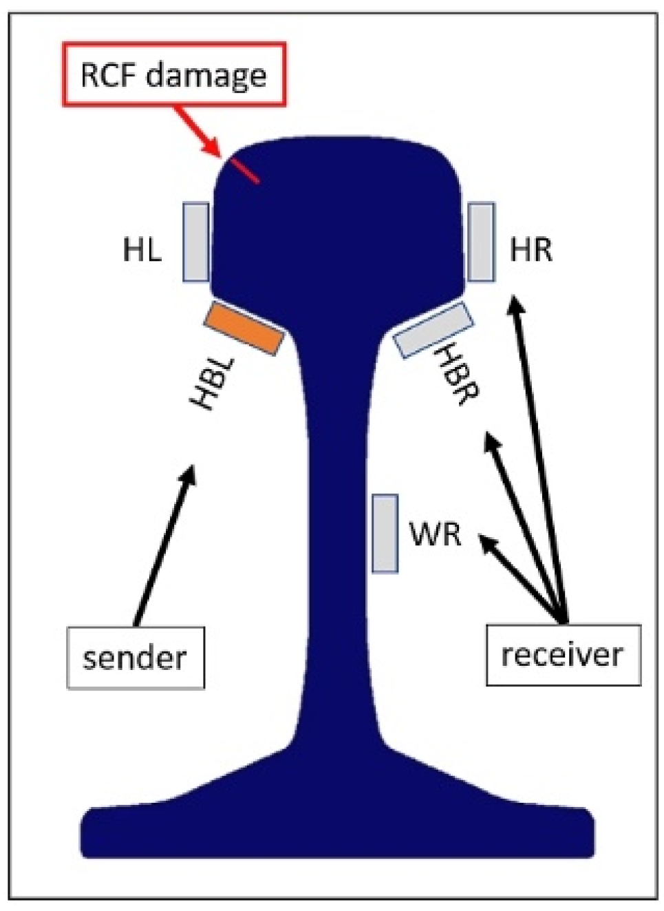
2.2. Pitch-Catch Setup for the Excitation and Measurement of Quasi-Rayleigh Waves with Contacting Transducers

In a recent publication, Masurkar et al. gave an overview on the advantages and disadvantages of contact and non-contact methods to excite and measure Rayleigh waves [7]; however, the literature cited therein only covers non-contact setups. As the aim of the present study was to test the ability to detect head checks using the SAW pitch-catch setup with transducers attached to the rail, i.e., aiming at wayside condition monitoring, the authors chose piezoelectric comb transducers in a pitch-catch setup. These transducers are widely used in nondestructive guided wave examinations, and are characterized by easy operation, low cost, and high sensitivity [7,8,9]. For signal excitation and measurement, the readily available commercial system gampt GS200 [9] was used.

The pitch-catch setup consisted of two piezo transducers combined with a comb adaptor to introduce and measure a narrowband surface acoustic wave with a center frequency of 1 MHz. In 2001 Danicki published a sketch of a similar comb transducer and detailed the wave generation theory behind it [10]. In the case of the gampt 1 MHz setup, the comb consisted of 10 contacting teeth with a spacing of 2.89 mm corresponding to a Rayleigh wave speed of 2889 m/s in aluminum.

The first experiments revealed that manually attaching the transducers to the rail (see Figure 2a) resulted in strong fluctuations in the excited and measured surface acoustic wave peak intensities, due to the fluctuating quantities of coupling agent between transducer and comb as well as between comb and rail. To improve the reproducibility of the signals, a transducer holder was designed that fixed the transducer on the rail via magnets, and controlled the contact pressure of the transducer to the rail via a spring, as shown in Figure 2b.

With the transducer holder shown in Figure 2b, the sending and the receiving transducers were placed on the rail as sketched in Figure 3. The sending transducer remained at the left bottom of the rail head (position HBL), whereas the receiving transducer was placed at different positions along the desired wave path (HL = head left, HR = head right, HBR = head bottom right, WR = web right). Note that in this sketch the corner cracks (head checks, see Figure 1) are on the left gauge corner of the rail. Consequently, the surface waves recorded at positions HR, HBR and WR correspond to surface waves that interacted with the head checks. Additionally, the amplitude of the surface wave at the left rail head (HL) before the damage location was measured and used to normalize the data at all sensing locations. The corresponding measurement procedure for a specific damage state took several minutes for each measurement. The main time factor was the careful placement of the comb transducers for sending and receiving. For a future setup closer to the desired in-track wayside condition monitoring, smaller SAW transducers will be fixed on positions where they are not endangered by the passing wheels (see Concluding Remarks).

The data was cleaned from unwanted noise by applying a narrow band pass filter with a center frequency of 1 MHz and a width of 0.2 MHz. For each sensing location the peak of the R-wave in the expected time window of wave arrival was extracted. The signal attenuation was computed with reference to the surface wave amplitude at the specific sensor locations (HR, HBR, WR) measured on the undamaged rail specimen.

2.3. Scattering of Rayleigh Waves at Surface Breaking Cracks—Theoretical Considerations

The scattering of elastic Rayleigh waves at surface breaking cracks, for idealized crack geometries (infinite half-space with a crack parallel to the surface normal) in the far field, has been solved analytically by Angel and Achenbach [11]. As shown in Figure 4, reflection, transmission and mode conversion from Rayleigh to bulk waves depend on the ratio of crack depth to wavelength $d/{\lambda }_R$ and the angle of incidence (where 0° means wave propagation perpendicular to the crack). Reflection, transmission and mode conversion are relatively independent of the angle of incidence for angles < 60°, cf. Figure 4a–c. Moreover, for small cracks ($d/{\lambda }_R$ < 1) the transmission coefficient is more sensitive to changes of crack length compared to the reflection coefficient. In general, the transmission coefficient is non-monotonous but has a monotonous region with high crack depth sensitivity for ratios $d/{\lambda }_R$ < 0.3, see Figure 4d.

As a first approximation, the wavelength of the Rayleigh waves in steel (with Young’s modulus E, Poisson’s ratio ν and mass density ρ, see

Table 1. Material parameters of the railway steel as input for the simulation.

Mass Density $\mathit{\rho }$	Young’s Modulus $\mathit{E}$	Poisson’s Ratio $\mathit{\mu }$
7800 kg/m³	200 GPa	0.29

) is given by $\lambda =\frac{v_R}{f}\approx \frac{\left(0.87+1.12\nu \right)v_S}{\left(1+\nu \right)f}\approx \frac{0.926 v_S}{f}\approx \frac{2920}{f}$, where the shear velocity is $v_S=\sqrt{G/\rho })\approx 3153 \mathrm{m}/\mathrm{s}$ for a shear modulus of $G=\frac{E}{2\cdot \left(1+\nu \right)}\approx$ 77.5 GPa. This corresponds to a wavelength of λ~2.9 mm at a frequency of f = 1 MHz. Thus, according to the considerations above, an unambiguous relationship between crack depth and transmission coefficient should be present for crack depths up to ~1 mm. Due to the insensitivity of the transmitted Rayleigh wave to the angle of incidence for the angles of interest (the inclination of the cracks with respect to the rolling direction is significantly smaller than 60°) it is sufficient to perform simulation studies on wave propagation in rail cross-sections for 2D geometries only.

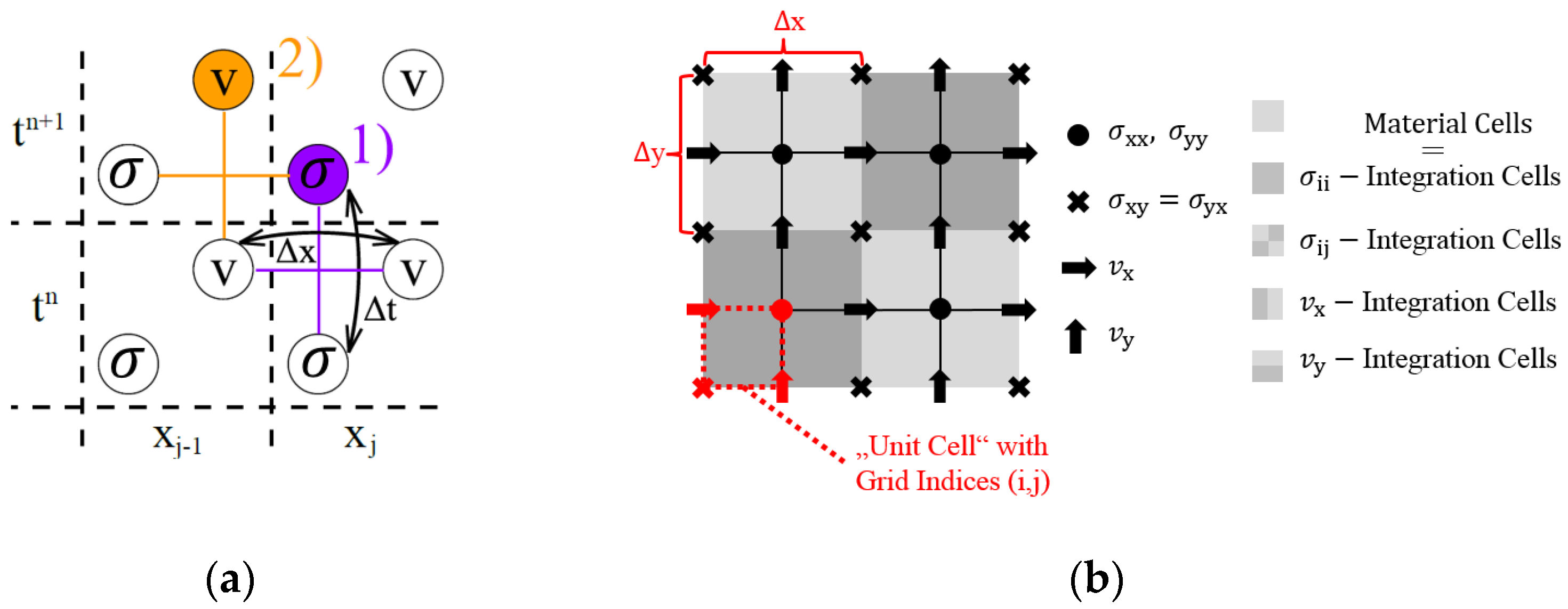
2.4. Simulation of Elastic Wave Propagation via EFIT

In contrast to the situation of an ideal surface crack in an ideal infinite material half-space, as discussed in the previous chapter, both the bulk waves generated by the transducer and those due to mode conversion at the crack can impede the detection of the reflected/transmitted surface acoustic wave intensities. To optimize the measurement setup and to clarify the wave propagation behavior, 2D and 3D elastodynamic finite integration technique (EFIT) software was developed and customized for the rail geometry. The elasto-dynamic equations in velocity-stress ($\stackrel{\rightharpoonup }{\mathrm{v}}$, σ) representation (consisting of the Cauchy momentum equation $\rho \frac{\partial \stackrel{\rightharpoonup }{v}}{\partial t}=\stackrel{\rightharpoonup }{\nabla }\cdot \mathsf{\sigma }$, together with the isotropic linear elastic material law $\dot{\mathsf{\sigma }}\approx E/\left[2\left(1+\mu \right)\right] tr(\dot{\mathsf{ϵ}})+2\mu \dot{\mathsf{ϵ}}$, where the linear strain rate is given by $\dot{\mathsf{ϵ}}\approx [(\stackrel{\rightharpoonup }{\nabla }\otimes \stackrel{\rightharpoonup }{\mathrm{v}})+{(\stackrel{\rightharpoonup }{\nabla }\otimes \stackrel{\rightharpoonup }{\mathrm{v}})}^T]/2$ and the material parameters Young’s modulus E and Poisson’s ratio μ are given in Table 1)were discretized on a staggered grid and the time evolution executed by an explicit update of the stress tensor and velocity vector in an alternating manner (leap-frog time integration, see Figure 5). For details on the corresponding theory and equations for the elastodynamic finite integration technique (EFIT) the interested reader is referred to the publication by Fellinger et al. [12]. A demonstration for a damped elastic wave simulation was recently published by Hammer et al. [13].

The software implementation was undertaken in Python using TensorFlow [14] as a tool for a convenient parallelization, enabling computation on multiple CPUs combined with GPU. The computations shown in this work, i.e., a 2D model of the rail cross-section, were performed using an Intel Xeon CPU E5-1650 v4 @ 3.60 GHz workstation with 6 cores and 30 GB RAM with a typical calculation and postprocessing time of ~22 h.

The rail geometries were drawn with the CAD package DraftSight and imported as a regular 2D cartesian grid with square edge length of 0.15 mm (i.e., a resolution of 20 grid points per wavelength) into the EFIT software. The values for the material parameters are listed in Table 1.

The initial conditions were a zero stress and velocity field in the whole domain. The excitation was implemented by setting a time-dependent velocity boundary condition at the location of the sending transducer—left bottom of the rail head (position HBL)—corresponding to the contact of the transducer comb (sender) with the rail body. The time dependence of the input signal was determined to match the waveform found experimentally. Three different crack constellations with 1–3 cracks, as shown in Figure 6, were used in the simulations. The geometry parameters of the investigated crack configurations were based on the examined thin section (shown later in Figure 18) taken at the experimental measurement location in the center of the artificially produced head check band, shown in Figure 1. The inclination with respect to the surface normal was ~103°. The spacing between the cracks amounted to 2 mm for the two-cracks layout and 1 mm for the three-cracks layout. The crack width was limited by the grid discretization and was equal to 0.3 mm. Additionally, the geometry without cracks was simulated as a reference basis.

3. Results

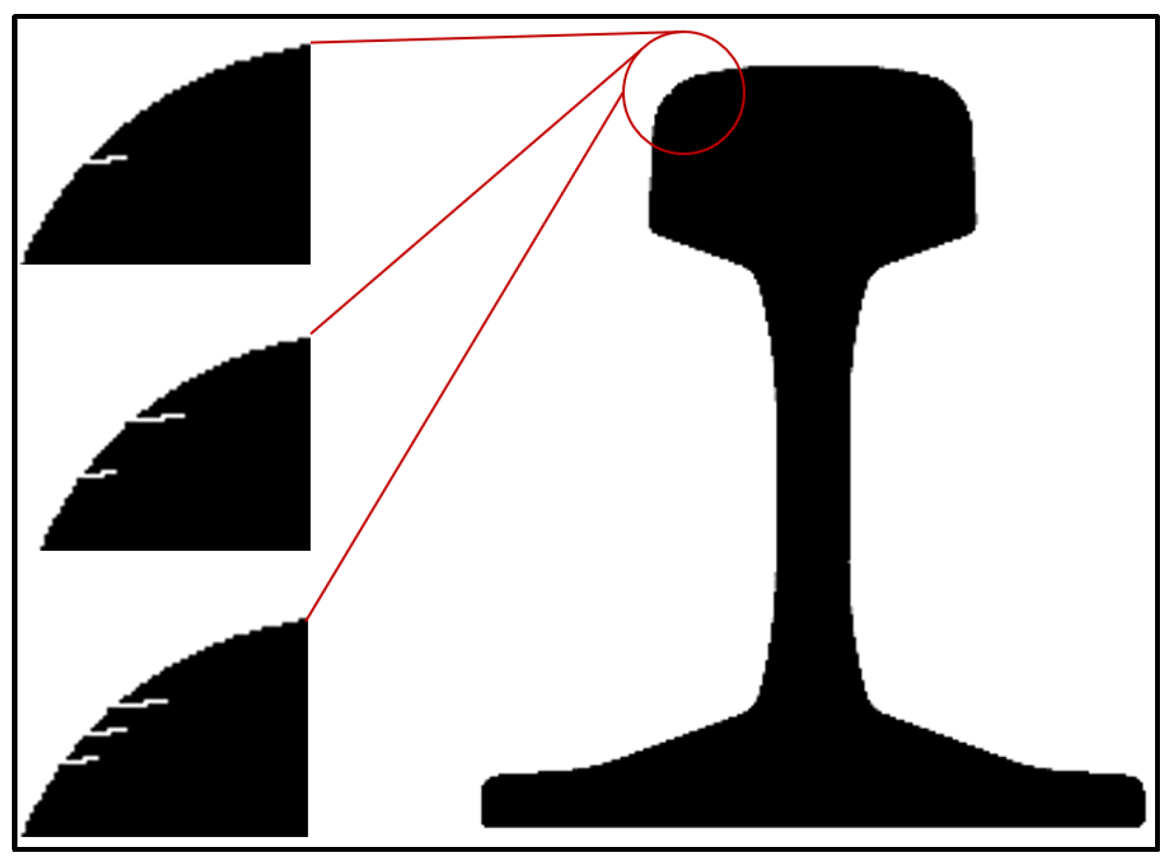
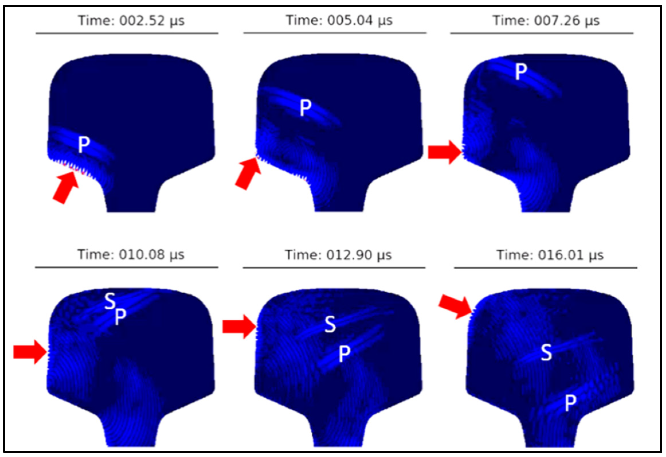
3.1. EFIT Visualization of Surface Wave Propagation in a Rail

The results of the numerical simulations provide a guidance for the signal processing, which is otherwise inconclusive if complex geometries, complex waveforms and mode conversions are involved. It is inevitable that simultaneously to the intended Rayleigh surface waves, bulk waves were also introduced by the comb transducer (sender) at the left bottom of the rail head. Figure 7 shows chronologically ordered snapshots of the magnitude of the velocity field over time. While the Rayleigh waves follow a simple path along the surface, the bulk waves show a complex behavior due to multiple scattering and mode conversion. In the first row a pressure wave (marked with “P”) is seen to propagate towards the top of the rail head. The oblique reflection leads to a partial conversion of the pressure wave into a shear wave (marked as “S”), as can be seen in the second row. The lower left figure at 10.08 μs shows an additional low-amplitude Rayleigh wave, caused by interference where the P- and the S-waves meet the surface. This is an example of the simulations conducted, which allowed optimization of the sender and receiver placement, so that the expected signal originating from interactions with the crack was well separated from undesired additional wave modes when arriving at the sensor. In the following, we examine in more detail the signals caused by these travelling waves at different positions of the rail head.

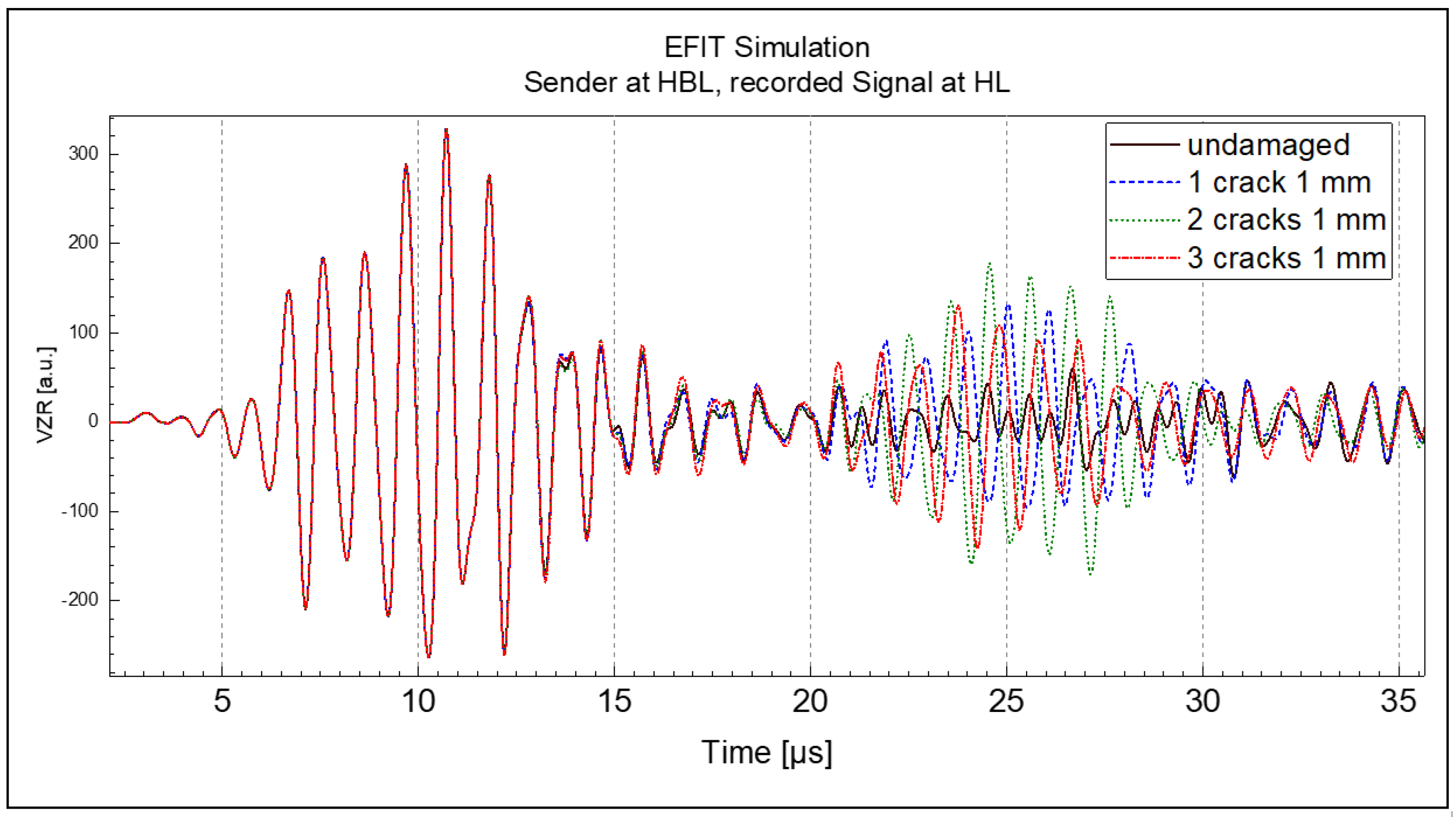
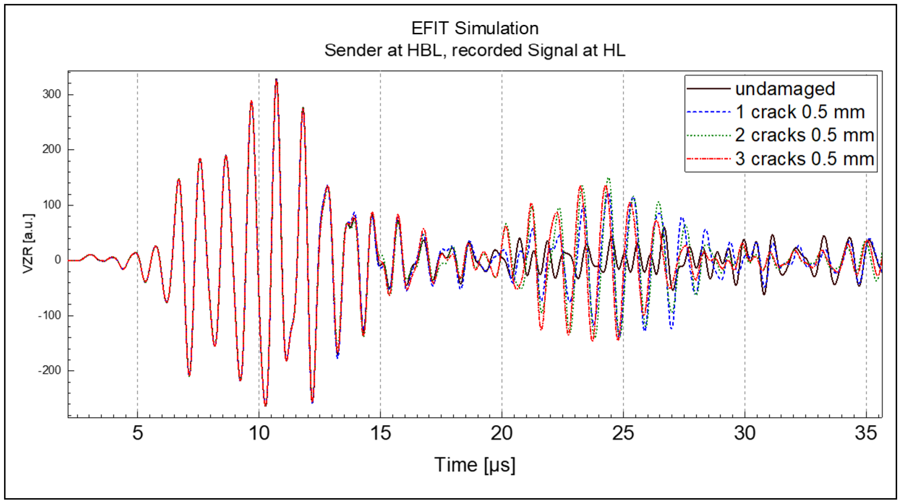
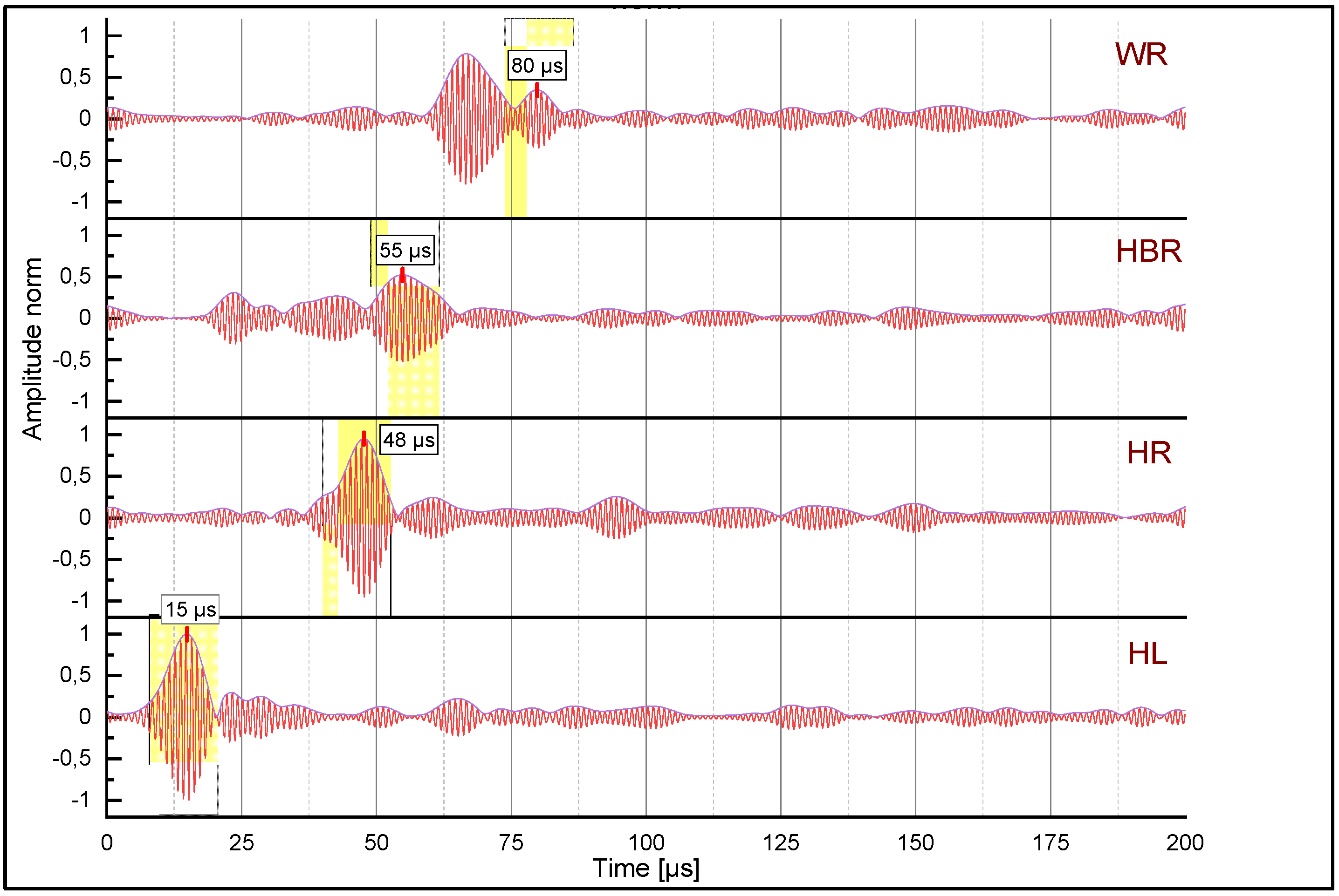
3.2. EFIT Calculation of the Wave Signals Received at Specific Cirumferential Points of the Rail–Wave Reflection

First, we investigated a setup with the receiver at the left side of the rail head just before the gauge corner (position HL), i.e., between the sender and the cracks; the receiver signal was thus expected to show first the wave coming from the sender, followed by the wave reflected at the cracks. In this setup the signal from the surface wave interaction with the cracks was well separated in time from bulk wave contributions. Figure 8 shows the simulated surface normal velocity component at position HL for the four crack configurations illustrated, viz., without cracks, with one, two, and three cracks, respectively. The passage of the pristine interrogation wave (initiating at 5 µs) and subsequent reflections of the surface wave (encircled in red) caused by the presence of the cracks can be clearly distinguished.

The proposed main factors influencing the reflected signal portion are the number of cracks and the crack depth with respect to the wavelength, whereas in these simulation studies the variations of crack inclination were neglected.

The simulation results in Figure 9 and Figure 10 show the waveform of the surface wave (first wave packet on the left side) followed by a signal generated by reflections at the cracks with different depth and crack numbers. Apart from subtle differences, the expectations from the theoretical considerations in Section 2.3 are confirmed: The amplitude of the reflection is not very sensitive in the range of crack lengths (see Figure 4d) of highest interest (e.g., 0.5–1 mm). Going beyond this statement, in the case of the longer cracks with 1 mm depth the reflected signal is to a high extent determined by the reflection at the first crack that the wave encounters. In comparisons, the reflected signals for the 0.5 mm cracks showed stronger differences between the one-, two-, and three-crack cases. The differences arise from the fact that in one case a single crack dominated the reflection, whereas in the other cases multiple cracks contributed to the reflected wave. In general, the reflected signal amplitude ranges for all simulation variants were in the same order of magnitude.

Overall, the simulations indicate that reflection is a less promising measurement arrangement, due to the complexity of the reflected signals and the difficulty identifying a clear correlation between crack depth and reflected signal amplitude.

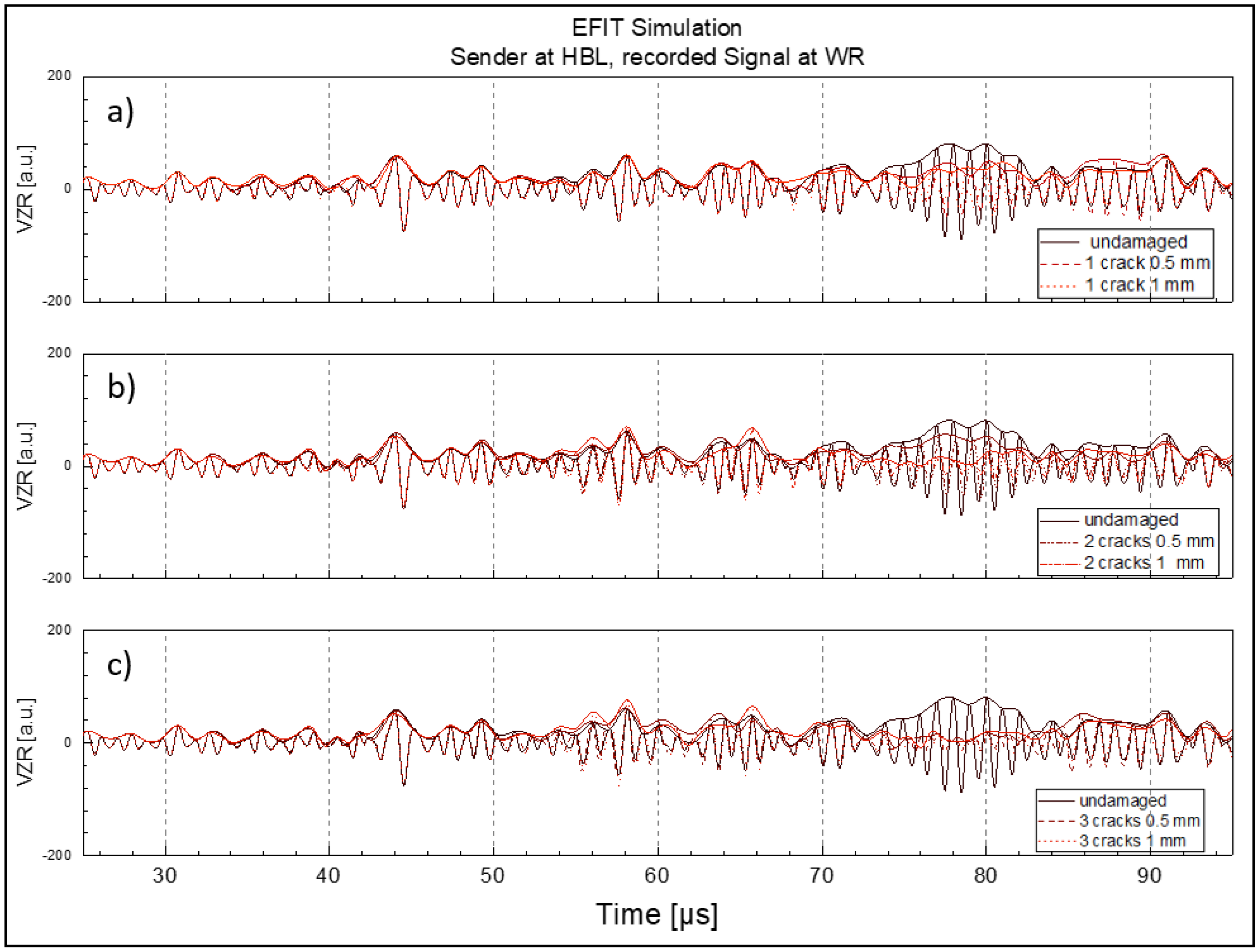
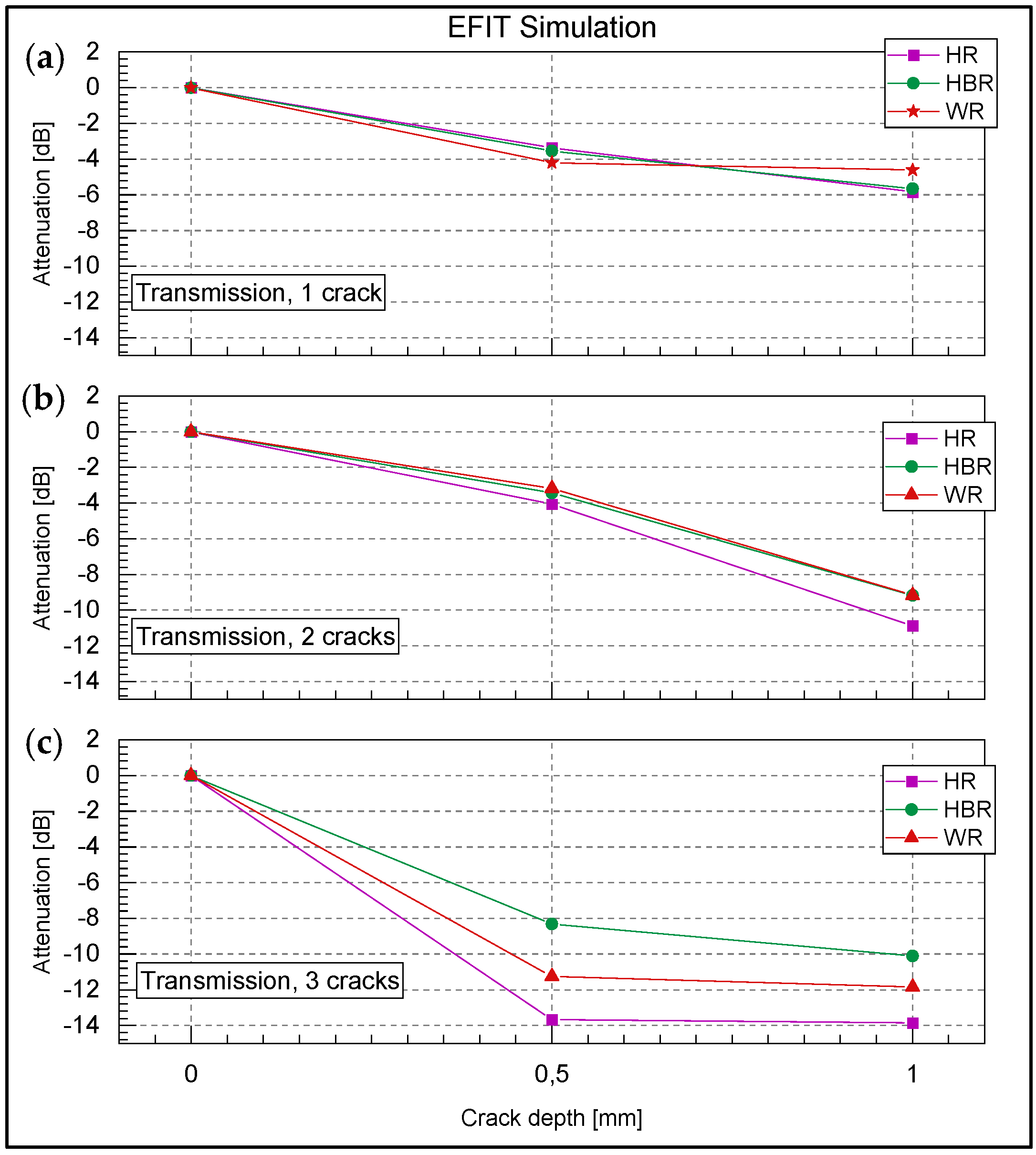
3.3. EFIT Calculation of the Wave Signals Received at Specific Cirumferential Points of the Rail–Wave Transmission

In terms of transmission, Figure 11, Figure 12 and Figure 13 show the simulated signals at positions HR (right side of the rail head), HBR (bottom right side of the rail head), and WR (right side of the rail web; cf. Figure 3 for the positions), respectively. Each figure is split into three subplots a, b and c illustrating the changes in the transmitted R-wave packets due to the interaction with different numbers of cracks, i.e., one crack (a, top), two cracks (b, middle), three cracks (c, bottom). The individual plots depict the surface normal velocities for the undamaged and damaged states with cracks of 0.5 mm and 1 mm depth. In addition to the individual signals, the envelope of each signal is shown, to indicate the change in the amplitude of the transmitted wave with different crack depths.

For all receiver locations the following can be deduced: With respect to R-wave packet width, the presence of a single crack (Figure 11, Figure 12 and Figure 13, plot a) did not hinder the identification of the wave packet for crack depths between 0.5 and 1 mm. The shape of the wave packet remains distinctive with a clear beginning and end. However, with increasing number of cracks (Figure 11, Figure 12 and Figure 13, plots b and c), the signal-to-noise ratio was reduced drastically and the R-wave packet in time became stretched and smeared. Regarding mode conversion of the R-wave packet at the crack faces and the subsequent occurrence of faster travelling bulk waves in the computed time signals, it can be seen in all plots that the initially coherent signals began to split ~18 µs before the arrival of the transmitted R-wave packet. The deviation of the signal envelopes naturally correlates with the number of cracks and depth, since the crack tips provide the appropriate centers for mode conversion.

To better compare the wave attenuation in transmission mode and possible effects due to receiver location, the results shown in Figure 11, Figure 12 and Figure 13 were condensed by extracting the attenuation of the envelope peak intensities with respect to the undamaged state for all receiver positions and damage states, plotted in Figure 14. Figure 14a shows a plot of the attenuation of the R-wave at the respective receiver positions due to a single crack at the rail gauge corner versus the crack depth. Figure 14b,c show the same type of plot for two and three cracks, respectively.

In general, the EFIT simulation results for R-wave transmission showed a stronger weakening of the signal for deeper cracks and for a higher number of cracks, but different trends can be noted:

Crack number and crack depth

The attenuation trends for the one-crack and two-crack models show similar behavior for all three sensing locations. For 0.5 mm crack depth, corresponding to a ratio $d/{\lambda }_R=0.17$, almost identical attenuation is observed for the one- and two-crack models. However, for a crack depth of 1 mm, i.e., a ratio $d/{\lambda }_R=0.3$, the two-crack model exhibits significantly higher attenuation than the one-crack model.

The presence of three cracks changes the picture fundamentally. Here, the attenuation values differ markedly between sensing locations for the shallower cracks of 0.5 mm depth; on the other hand, for each individual location the attenuation barely changes between 0.5 mm and 1 mm crack depth.

Receiver position

Generally speaking, when examining Figure 11, Figure 12 and Figure 13, the R-wave packet sensed at the right rail head (location HR, Figure 11) shows the most distinct shape compared with the sensing locations below the rail head (location HBR, Figure 12) and web (location WR, Figure 13). This is due to increasing signal overlaps caused by rail-geometry-born reflections. This can also be observed for the increase in noise level with increasing sensing distance. Looking at Figure 14 it can be noted that the R-wave attenuation was strongest at the HR sensing location, especially with an increasing number of cracks; a logical consequence of the higher signal-to-noise ratio and less overlap of mode converted bulk waves at this location. The strong attenuation in the case of the three-crack model and bad signal-to-noise ratio (i.e., signal interference) at the farther sensing locations led to lower attenuation values there.

3.4. Measured Wave Signals Recorded at Specific Cirumferential Points of the Rail–Wave Transmission

Figure 15 and Figure 16 show plots of the signals measured with the gampt setup (described in Section 2.2) at the four sensor locations illustrated in Figure 3. Due to the narrow-band signal characteristic of the actuator, a band-pass filter with a center frequency of 1 MHz and a bandwidth of 0.2 MHz was used to clean the recorded signals of unwanted noise. The measurements in Figure 15 were taken before the rail was subjected to the loading cycles at the wheel–rail test rig; Figure 16 represents the measurements at the end of the rolling contact fatigue experiment after 310,000 loading cycles. These signals illustrate the propagation of a surface wave along the rail circumference in an undamaged and a damaged rail, respectively. Again, the actuator was located at the left rail head bottom. The distinction between the main surface wave packet, and other surface and bulk waves due to reflections, is based on the velocity of the main/direct surface wave and thus on its position on the time axis (that changed only slightly due to the manual positioning of the transducers for each measurement). Correspondingly, the occurrence of the surface wave at the individual sensor locations is indicated by a yellow box. All signals were normalized with respect to the peak value of the first wave packet at sensor position HL occurring at ~15 µs, which represents the interrogation wave before it hit the gauge corner (and the eventual head checks there). This normalization implies that the surface wave that always overlapped with other waves (reflections, bulk waves) was the main wave component to interact with the surface cracks, whereas any corresponding interaction of reflected waves and bulk waves can be considered negligible. The latter was also confirmed by the simulation studies where the individual reflections can be traced.

All surface wave packets recorded at the follow-up locations experienced attenuation with increasing travelling distance, and possible presence of surface defects with increasing number of load cycles. In addition to the dominant peak of the surface wave, numerous rail-geometry dependent reflections can be noted. Due to the repeated manual procedure of sensor placement at the individual locations, sensor positions were not completely identical for measurements at different loading cycles. Therefore, surface wave arrival times varied slightly and were not used for further analyses. Instead, the shape and amplitude of the time signals were compared and related to head check formation.

Comparing the signals recorded at the rail head positions HL and HR shown in Figure 15 and Figure 16, respectively, it can be noted that the signal-to-noise ratio increased with the number of load cycles. An explanation for this phenomenon might be that the initially rough surface of the pristine rail was reduced by the repeated passage of the test wheel.

Looking at the measurements for the damaged state in Figure 16, it can be recognized that the shape of the surface wave packet became more and more elongated with increasing travelling distance and hence harder to detect; this is especially true for sensing location WR, where the distortion is so pronounced that the peak of the R-wave signal disappeared completely.

4. Discussion

To analyze the evolution of the wave attenuation due to RCF damage, the observed peak amplitudes (as illustrated in Figure 15 for the pristine state and in Figure 16 for the state after 310,000 wheel passes) were extracted and normalized to the undamaged peak at the sensing location, see Figure 17. It can be seen that the sensors at positions HR (head right) and HBR (head bottom right) showed increasing attenuation, i.e., decreasing signal peak values, with increasing number of load cycles (wheel passes). Position WR (web right) has not been evaluated due to the difficulties in detecting the peak of the extremely distorted wave packet, cf. Figure 16. A linear regression analysis gave slopes of (−2.12 ± 0.17) × 10⁻⁵ and (−1.87 ± 0.32) × 10⁻⁵ dB/cycle for positions HR and HBR, respectively (estimate ± standard deviation for the slope). The associated significance values p of 5.92 × 10⁻⁶ and 6.38 × 10⁻⁴ from the t-statistic corroborate from a statistical point of view the hypothesis of a clear negative correlation between the number of wheel passes and the attenuation of the surface acoustic waves (p << 0.05).

From a physical point of view, this behavior is related to the development of the head checks.

Figure 18 shows a thin section of the rail gauge corner taken at the end of the RCF experiment after 310,000 load cycles (wheel passes) at the measurement cross-section, displaying a pronounced head check pattern. The average depth of these cracks amounted to 0.62 mm, giving a ratio of $\mathrm{d}/{\mathsf{\lambda }}_{\mathrm{R}}\approx$ 0.62 mm/2.9 mm $\approx$ 0.21. At that time, an attenuation of −6.5 dB can be read from Figure 17, which corresponds to a transmission coefficient of $\approx$0.47. This agrees reasonably well with our 2D EFIT simulation results for two cracks, Figure 14b, and with the theoretical results from Angel and Achenbach [11], cf. the plot of attenuation vs. $\mathrm{d}/{\mathsf{\lambda }}_{\mathrm{R}}$ in Figure 4e.

As it is clearly impossible to mount a permanent sensor on the side of the rail head, the technologically relevant sensor position for future condition monitoring applications is the head bottom (position HBR). Compared to position HR, the absolute value of the slope of the trend line is slightly smaller, and the residual standard deviation SD of the regression analysis is somewhat higher (0.872 vs. 0.506 dB). Still, the ±2 × SD scatter bands corresponding to a statistical coverage of about 95% overlap almost entirely, making position HBR an adequate choice for future applications.

5. Concluding Remarks

In the present contribution it has been demonstrated by means of simulation and experiment that rail gauge corner cracks (head checks) can be detected by surface acoustic waves with a frequency of 1 MHz. In a pitch-catch setup, the attenuation correlates with crack depth if the excitation frequency is chosen appropriately according to the depth range of interest. This correlation was demonstrated by a series of measurements during a rolling contact fatigue test where head checks developed; attenuation due to crack depth measured at the end of the test agreed reasonably well with simulation results and theoretical results from the literature.

In order to proceed from crack detection to crack-depth measurement, the method needs to be calibrated so that the depth of the head checks can be reliably deduced from the measured attenuation. To this purpose, extensive experimental testing will be necessary, with individual tests being terminated after different numbers of cycles and thin sections being taken (the most reliable, albeit destructive, method of crack-depth measurement). Additional challenges are the dependence of the attenuation on crack numbers and crack spacing, which has been already briefly addressed in the present work, and a possible dependence on the microstructure of the material (rail grade).

As it was revealed that the repeated application of the transducers led to additional experimental scatter, this method is recommended mainly for a permanent sensor setup at selected track locations. Hence, the SAW excitation and measurement setup with transducers fixed on the rail will be the next step towards wayside condition monitoring using SAW. A fixed mounting of smaller SAW transducers will improve the reproducibility and hence the scatter of the data. Due to the reduction of influence from manually attaching the transducer for each measurement (see Section 2.2), the identification of the desired surface wave component on the time axis will be easier. In this way it is expected not only that head check formation can be detected at the earliest stage, but also that crack depth development can be monitored closely over time, thereby providing important information for maintenance scheduling in a condition-based maintenance concept.

In the early stages of crack formation, with cracks less than approx. 0.1 mm in length, rust, surface roughness and changes in rail geometry due to abrasive wear could influence the SAW signals and prevent clear distinction between these changes and the onset of crack formation. However, the simulation and measurement results indicate that cracks exceeding a length of about 0.5 mm should be clearly detectable with SAW in the proposed frequency range.

Our eventual aim is wayside condition monitoring with inexpensive, small and reliable transducers implemented in or attached to the rails at “hotspots” on the railway network. This is intrinsically different to the EMAT-based scanning approach, e.g., as proposed in ref. [15], because our application implies finding the sending and receiving positions on the rail where the wheel passage allows it, i.e., on the rail sections below the running band. Furthermore, our numerical and experimental results indicate that it is not sufficient to use specimens with single cracks or artificial slots to calibrate a condition monitoring device for depth measurements of head checks in track, because these gauge corner cracks usually evolve as crack networks rather than single cracks.

References

1. Eadie, D.; Elvidge, D.; Oldknow, K.; Stock, R.; Pointner, P.; Kalousek, J.; Klauser, P. The effects of top of rail friction modifier on wear and rolling contact fatigue: Full-scale rail–wheel test rig evaluation, analysis and modelling. Wear 2008, 265, 1222–1230. [Google Scholar] [CrossRef]
2. Kostrzewski, M.; Melnik, R. Condition Monitoring of Rail Transport Systems: A Bibliometric Performance Analysis and Systematic Literature Review. Sensors 2021, 21, 4710. [Google Scholar] [CrossRef] [PubMed]
3. Chen, K.; Fu, X.; Dorantes-Gonzalez, D.J.; Li, Y.; Wu, S.; Hu, X. Laser-Generated Surface Acoustic Wave Technique for Crack Monitoring—A Review. Int. J. Autom. Technol. 2013, 7, 211–220. [Google Scholar] [CrossRef]
4. Masserey, B.; Raemy, C.; Fromme, P. High-frequency guided ultrasonic waves for hidden defect detection in multi-layered aircraft structures. Ultrasonics 2014, 54, 1720–1728. [Google Scholar] [CrossRef] [PubMed] [Green Version]
5. Thompson, R.-B. Physical Principles of Measurements with EMAT Transducers. Phys. Acoust. 1990, 19, 157–200. [Google Scholar] [CrossRef]
6. Hribšek, M.F.; Tosic, D.V.; Radosavljević, M.R. Surface Acoustic Wave Sensors in Mechanical Engineering. FME Trans. 2010, 38, 11–18. Available online: https://www.mas.bg.ac.rs/_media/istrazivanje/fme/vol38/1/02_mfhribsek.pdf (accessed on 1 February 2022).
7. Masurkar, F.; Rostami, J.; Tse, P. Design of an innovative and self-adaptive-smart algorithm to investigate the structural integrity of a rail track using Rayleigh waves emitted and sensed by a fully non-contact laser transduction system. Appl. Acoust. 2020, 166, 107354. [Google Scholar] [CrossRef]
8. Stock, R.; Pippan, R. Rail grade dependent damage behaviour—Characteristics and damage formation hypothesis. Wear 2014, 314, 44–50. [Google Scholar] [CrossRef]
9. Ultraschall Echoskop GS200. Available online: https://www.gampt.de/en/product/ultraschall-echoskop-gs200 (accessed on 1 February 2022).
10. Danicki, E.J. Scattering by periodic cracks and theory of comb transducers. Wave Motion 2002, 35, 355–370. [Google Scholar] [CrossRef]
11. Angel, Y.C.; Achenbach, J.D. Reflection and transmission of obliquely incident Rayleigh waves by a surface-breaking crack. J. Acoust. Soc. Am. 1984, 75, 313. [Google Scholar] [CrossRef]
12. Fellinger, P.; Marklein, R.; Langenberg, K.J.; Klaholz, S. Numerical modeling of elastic wave propagation and scattering with EFIT—Elastodynamic finite integration technique. Wave Motion 1995, 21, 47–66. [Google Scholar] [CrossRef]
13. Hammer, R.; Mitterhuber, L.; Brunner, R. Phasor Wave-Field Simulation Providing Direct Access to Instantaneous Frequency: A Demonstration for a Damped Elastic Wave Simulation. Acoustics 2021, 3, 485–492. [Google Scholar] [CrossRef]
14. TensorFlow. Available online: https://www.tensorflow.org/ (accessed on 8 June 2022).
15. Edwards, R.S.; Dixon, S.; Jian, X. Depth gauging of defects using low frequency wideband Rayleigh waves. Ultrasonics 2006, 44, 93–98. [Google Scholar] [CrossRef] [PubMed]
Figure 1. Head check pattern achieved at the end of the RCF experiment in the 1:1 wheel–rail test rig at voestalpine (scales are in cm).
Applsci 12 06334 g001
Figure 2. Images of the Rayleigh wave (R-wave) transducers: manual attachment of the Rayleigh wave transducer (a), design of a holder that fixes the transducer with constant pressure to the rail (b).
Applsci 12 06334 g002
Figure 3. Sketch illustrating the positions of SAW sender and receiver with respect to the rail damage location. Explanations of the abbreviations are given in the text.
Applsci 12 06334 g003
Figure 4. Theoretical results for the scattering of Rayleigh waves at a surface breaking crack (data taken from Angel and Achenbach 1984 [11], for a Poisson’s ratio ν = 0.3. Reflection (a), transmission (b), energy conversion to bulk waves (c) depending on the angle of incidence, as well as reflection (d) and transmission (e) as a function of crack depth d divided by the wavelength λ R .
Applsci 12 06334 g004
Figure 5. (a) Leap-frog time integration of the elastodynamic equations. (b) Spatial grid by staggering stress tensor σ i j and velocity vector components v i (reprinted from [13]).
Applsci 12 06334 g005
Figure 6. Three different crack geometries as modelled in the simulations. The rail cross-section corresponds to the standard 60E1 (UIC60) profile (EN 13674–1).
Applsci 12 06334 g006
Figure 7. Simulated ultrasonic wave propagation in an undamaged rail head after introducing a wave corresponding to excitation with a comb transducer. The magnitude of the velocity field is shown for subsequent snapshots in time. The red arrow marks the position of the Rayleigh wave, “P” marks the pressure wave and “S” stands for the shear wave.
Applsci 12 06334 g007
Figure 8. Simulated signal as received at position HL, without crack, and due to reflection at 1 crack, 2 cracks, and 3 cracks, respectively. The crack depth as shown in the sketch is 0.5 mm. The red circles mark the part of the signal coming from the interaction with the cracks. v denotes the velocity component at the receiver position, projected to the surface normal.
Applsci 12 06334 g008
Figure 9. EFIT simulation surface normal velocity signal recorded at HL, crack depth 1 mm.
Applsci 12 06334 g009
Figure 10. EFIT simulation surface normal velocity signal recorded at HL, crack depth 0.5 mm.
Applsci 12 06334 g010
Figure 11. Change of transmitted R-wave received at position HR with increasing number of cracks and crack depths up to 1 mm; (a) 1 crack (b) 2 cracks (c) 3 cracks.
Applsci 12 06334 g011
Figure 12. Change of transmitted R-wave received at position HBR with increasing number of cracks and crack depths up to 1 mm; (a) 1 crack (b) 2 cracks (c) 3 cracks.
Applsci 12 06334 g012
Figure 13. Change of transmitted R-wave received at position WR with increasing number of cracks and crack depths up to 1 mm; (a) 1 crack (b) 2 cracks (c) 3 cracks.
Applsci 12 06334 g013
Figure 14. Attenuation of transmitted R-wave with respect to the undamaged state depending on crack depth, number of cracks and receiver location; (a) for 1 crack, (b) 2 cracks, (c) 3 cracks.
Applsci 12 06334 g014
Figure 15. Signals measured along rail circumferential positions (HL, HR, HBR, WR) on the undamaged rail, normalized with respect to the peak amplitude at position HL.
Applsci 12 06334 g015
Figure 16. Signals measured along rail circumferential positions (HL, HR, HBR, WR) on the rail with severe head check damage after 310,000 load cycles, normalized with respect to the peak amplitude at position HL.
Applsci 12 06334 g016
Figure 17. Evolution of measured signal amplitudes over cycle number for sender at position HBL and receiver in transmission mode at the positions HR and HBR, with linear regression curves for each position (mean curves solid, ±2 standard deviation curves dashed).
Applsci 12 06334 g017
Figure 18. Thin section of rail gauge corner (perpendicular to the running direction of the wheel to match the simulations sketched in Figure 8) taken after 310,000 load cycles (wheel passes) at the measurement cross-section, (a) head checks with 0.62 mm depth, (b) detailed view.
Applsci 12 06334 g018