Shape-Based Breast Lesion Classification Using Digital Tomosynthesis Images: The Role of Explainable Artificial Intelligence

Abstract

Computer-aided diagnosis (CAD) systems can help radiologists in numerous medical tasks including classification and staging of the various diseases. The 3D tomosynthesis imaging technique adds value to the CAD systems in diagnosis and classification of the breast lesions. Several convolutional neural network (CNN) architectures have been proposed to classify the lesion shapes to the respective classes using a similar imaging method. However, not only is the black box nature of these CNN models questionable in the healthcare domain, but so is the morphological-based cancer classification, concerning the clinicians. As a result, this study proposes both a mathematically and visually explainable deep-learning-driven multiclass shape-based classification framework for the tomosynthesis breast lesion images. In this study, authors exploit eight pretrained CNN architectures for the classification task on the previously extracted regions of interests images containing the lesions. Additionally, the study also unleashes the black box nature of the deep learning models using two well-known perceptive explainable artificial intelligence (XAI) algorithms including Grad-CAM and LIME. Moreover, two mathematical-structure-based interpretability techniques, i.e., t-SNE and UMAP, are employed to investigate the pretrained models’ behavior towards multiclass feature clustering. The experimental results of the classification task validate the applicability of the proposed framework by yielding the mean area under the curve of 98.2%. The explanability study validates the applicability of all employed methods, mainly emphasizing the pros and cons of both Grad-CAM and LIME methods that can provide useful insights towards explainable CAD systems.

1. Introduction

Breast cancer, which is the second most widespread cancer among women worldwide, has turned into global public health issue due to its complex intrinsic aetiology [1]. The early diagnosis and monitoring of the cancer significantly reduces the death risks, leads to better prognosis and therapy, and lowers the treatment cost.

Mammography wears the crown of being the gold standard among several imaging modalities because it offers the potential of early detection of pathology [2]. However, mammography is a 2D method that reduces the ability to visualize lesions in case of prevalent glandular component in dense breast. Moreover, the mammography represents a 2D projection of a 3D structure for which, geometrically, tissues belonging to different planes are superimposed in the radiographic image.

Other imaging techniques including magnetic resonance (MR), computed tomography (CT), and digital breast tomosynthesis (DBT) are strong candidates where in-depth analysis of hazardous cases is required. Among these, the DBT is proven to have higher accuracy with respect to the 2D imaging methods [3]. After acquisition of the multiple thin and high-resolution images, the DBT system produces a quasi-three-dimensional format of the reconstructed breast images aiming to reduce the effect of tissue superimposition.

Moreover, the required radiation dose is not high, contrary to the conventional imaging techniques, and the generated images appear to have greater resolution and contrast [4]. The DBT represents a more accurate diagnostic indicator than 2D imaging for evaluating the morphological features, e.g., shape and margin of the different immunophenotypes of the breast cancer, thus being able to play a crucial role in the molecular imaging and prognosis [5,6,7,8,9].

Over the last decade, deep learning (DL) has emerged as a promising computational approach for the automatic detection, classification, and segmentation of cancerous masses thorough the analysis of diagnostic medical images, thus enabling the computer-aided diagnosis (CAD) and clinical decision support systems [10,11,12,13]. The DL methods along with the traditional image processing techniques have already been established as an effective approach to automatically analyze diagnostic images for breast cancer diagnosis and monitoring [3,14,15]. Numerous studies dealt with automatic detection, segmentation, and classification of the breast lesions that achieved considerably moderate to high performances [16,17,18,19,20,21,22,23,24,25]. However, the automatic classification of the breast lesions according to shape, size, and physical appearance remains a challenging task due to the varying shape that refers to different type and stage of the cancer [26] (see Figure 1). The breast cancer is morphologically categorized into several varying shapes based on cancer growth pattern, named as round, oval, lobulated, irregular, and architectural distortion [27,28].

Numerous existing studies deal with the shape-based breast cancer classification [26,29,30]; however, most of these consider the mammogram instead of the DBT that offers several advantages as discussed above. A deep discussion of the state of the art is presented in Section 2. In spite of the enormous success, the complex nature of the DL techniques hides any possible information of the underlying decision mechanism [31,32], which questions its usage in the healthcare domain where explainability holds paramount significance to build a trust on decisions made by surging artificial intelligence (AI). Explainable artificial intelligence (XAI) brings forward the possibility of explaining the results of DL models and reveals how the models produce these results. Generally, XAI is supposed to fit a model onto four basic attributes [33]:

• Transparent: open to the degree where humans can understand the decision-making mechanism.
• Justifiable: the decision can be supported or justified along each step.
• Informative: to provide reasoning and allow reasoning.
• Uncertainty yielding: does not follow hard-coded structure, but open to change.

XAI has drawn a tremendous amount of attention in the recent past (see Figure 2) and it is not hard to comprehend the importance of such methodologies in the clinical field where AI is spreading fast [34]. Such new research topic is extremely fascinating yet challenging, because as it can be easily envisaged, a more complex AI model that can reach high-level performance is less interpretable than, for example, a simple rule-based model (see Figure 3).

Numerous XAI methods and relative updated versions have been proposed in the literature [34]. The presented approaches can be classified into two major categories: perceptive interpretability and mathematical interpretability. The former includes interpretabilities that can be visually perceived by humans, for example, the heatmaps that report the importance of input components in their contribution to that decision. The mathematical-interpretability-based methods usually rely on very easy models, e.g., linear models, or on correlation/clustering methods that analyze the extracted features. When visual evidence is not useful or erroneous, the mathematical evidence can also be used as a complement for the interpretability. Therefore, various methods should be applied simultaneously for the sake of providing reliable interpretability [35].

A limited number of studies on shape-based classification of the breast lesion images dealt with the explainability of the trained DL models [36,37]. However, all the revised studies exclusively consider the same single method and binary classification that, in most of the cases, is related to malignant vs. benign lesion classification. A deep discussion of the state of the art is presented in Section 2.

In this study, the authors develop and validate a convolutional neural network (CNN)-based DL framework for the classification of breast lesions according to the shape by analyzing the related region of interest (RoI) on DBT images. Considering the shapes of cancerous masses, the breast imaging reporting and data system (BIRADS) classification of the American College of Radiology, which is the most commonly employed in the clinical and digital breast tomosynthesis settings, has been considered [38]. Such kind of taxonomy refers to the following three classes (see Figure 4):

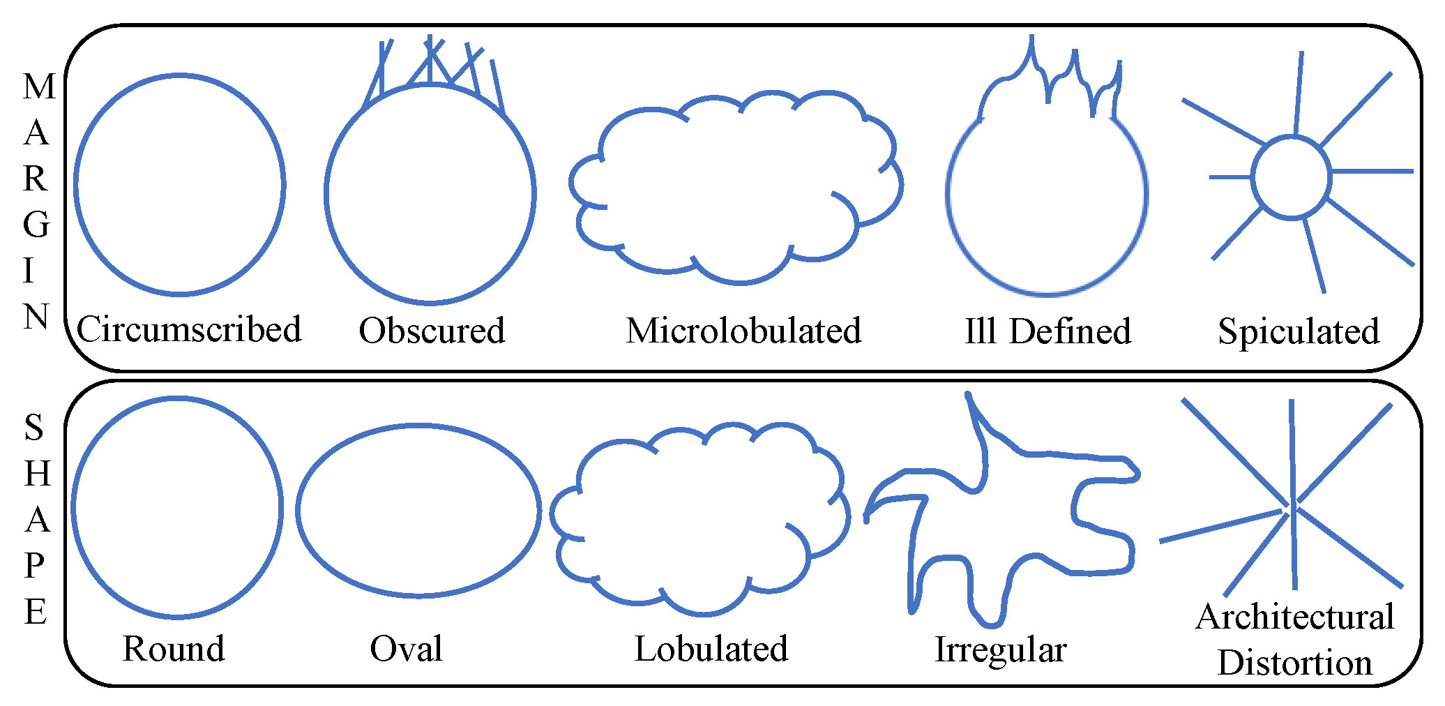
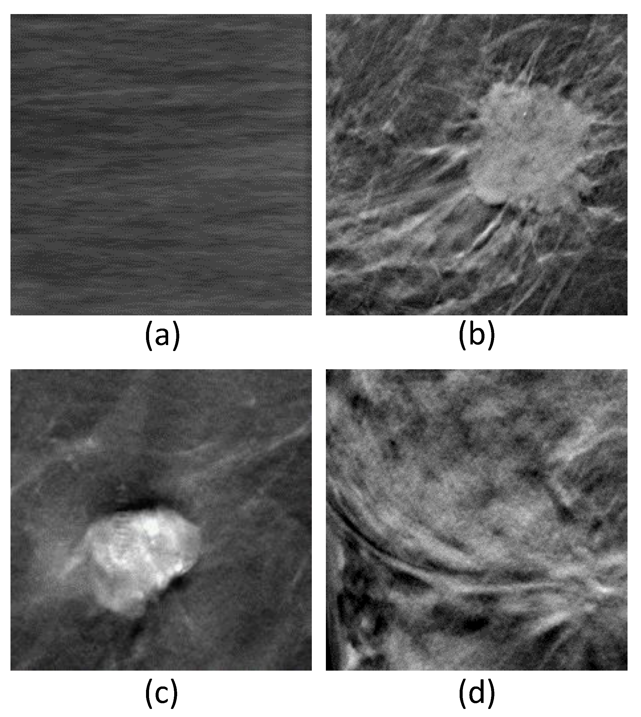
• Regular opacity (Oro) which includes the round, oval, and lobulated shapes;
• Irregular opacity (Ori);
• Architectural distortion shape (Ost).

The clinical importance of the three BIRADS classes consists of the possibility of identifying regular masses or irregular masses/architectural distortions which is the principal purpose of the clinical breast setting for early diagnosis of breast cancer. In fact, it is well known that the Oro lesions are usually benign, whereas Ori and Ost lesions are malignant. Finally, it is also worth mentioning that in this study the None class, i.e., images that do not contain any lesion, is also included (see Figure 4).

Moreover, the study employs eight state-of-the-art pretrained CNN architectures that have been compared both with and without fine-tuning. Two different online data augmentation routines have been tested to study the impact of several augmentation methods on the performances. The dataset used in this study comes from authors’ previous study and comprises 39 breast DBT exams of 16 patients. Interested readers are kindly referred to such study to explore more about the data acquisition and composition [39].

The trained DL models and related results have been further interpreted, employing two different methodologies for each of the two explanation mechanisms. Gradient-weighted class activation mapping (Grad-CAM) method and local interpretable model-agnostic explanations (LIME) have been used to visually interpret the results, whereas t-distributed stochastic neighbor embedding (t-SNE) and uniform manifold approximation and projection (UMAP) techniques have been utilized to study the mathematical interpretability of the features automatically extracted by all eight CNN architectures [34].

The remainder of the article is organized as follows: studies related to the shape-based cancer classification and the breast cancer explainability are presented in Section 2; Section 3 comprises materials exerted in the study and provides the comprehensive details about the employed methods; results are described in Section 4 and further discussed comprehensively in Section 5; Section 6 highlights the shortcomings and offers a future perspective of the study for potential research community; finally, the article concludes by making the final remarks in Section 7.

2. Related Studies

Over the last decade, because of the superior aptitude to capture cancers, the DBT has become the new gold standard for the digital mastography [40]. Alongside this, machine learning has revolutionized the medical field by offering automatic detection, segmentation, and classification of the cancer [24,25,41,42,43,44].

Moreover, XAI has additionally elevated the confidence of the research community to apply DL in the computer-assisted treatments [34] by uncovering the black box and hidden nature of the DL. This helps building confidence on the usage of AI in clinical settings, also paving the way towards the DL-centered image-guided CAD systems.

This section presents and discusses the most relevant and original studies dealing with automatic breast cancer classification and the incorporation of the XAI techniques on the breast cancer imaging recently.

The shape of the breast tumors leads to diagnosis of the different types and stages of the cancer [26]. Generally, the breast cancer is morphologically categorized into five shapes based on tumor growth pattern, named round, oval, lobulated, irregular, and stellar [27], as depicted in Figure 1. Numerous authors claim that the transition from the round shape to stellar shape of the cancer is the journey from benign to malignant cancer [26,29,45].

The shape-based breast cancer classification of mammogram images at RoI level using generative adversarial network (GAN) and CNN is presented by Singh et al. [29]. The authors used a publicly available dataset for validation and achieved an overall classification accuracy of 80% for irregular, lobular, oval, and round shape classes.

Similarly, Kisilev et al. [28] proposed a multi-task loss CNN architecture based on the Faster R-CNN model to detect tumor lesions by considering irregular, round, and oval shapes of the breast cancerous lesions using in-house and publicly available datasets. Their approach generated bounding boxes around the tumor, and then used the semantic descriptors to identify the lesion shape inside the RoI. The accuracy on in-house and public datasets reached 88% and 82%, respectively, where both accuracy values were computed on accurately labeled data for testing purposes.

In a previous study by authors [39], two different approaches for the classification of DBT images into four lesions, i.e., irregular opacity, regular opacity, stellar opacity lesions, and no lesions, were implemented and tested on an in-house dataset. The first approach utilizes an artificial neural network that takes morphological and hand-crafted features extracted from the RoI images and performs classification. The second framework encompasses the pretrained CNNs without requiring the hand-crafted features. The authors claimed that the VGG network outperformed the other pretrained architectures by reaching 91.61% and 81.49% accuracy with and without augmentation.

A GAN-based interpretable CAD system for the classification of oval, round, irregular, and lobular shapes on the mammogram images was devised by Kim et al. [30]. The CAD system was tested on a public dataset that managed to achieve 71% accuracy on the lesion shape classification.

A study on mammogram and MR scans on three publicly available datasets was conducted by Shrivastava et al. [26] to classify the shapes of the tumorous regions using geometrical feature-based classifier. Since the authors merely considered the binary classification problem (benign lesion vs. malignant lesion), unlike previously explained methods, the reported accuracy, i.e., 91.4%, was pretty high.

A recent study by Sakai et al. used SVM, random forests, naive Bayes, and multilayer perceptron methods to classify the breast lesions on tomosynthesis images [46]. The authors also considered radiomic features along with the shape of the lesion. All the round and oval tumors were labeled benign, whereas the irregular and the stellar were labeled malignant on an in-house dataset. The best achieved accuracy value was 55% for round vs. oval classification, and 84% in case of irregular vs. stellar classification.

Said et al. [47] adopted the genetic algorithm to select the most significant hand-crafted features out of the total 130. Finally, the back-propagation neural network was employed for the classification task on round, oval, lobular, and irregular shapes that reached 84.5% accuracy on the digital database for screening mammography dataset.

Several studies in the literature dealt with the breast cancer imaging and XAI. Ricciardi et al. proposed a binary classification framework based on AlexNet and VGG-19 architectures to recognize the presence or absence of mass lesion on DBT image of two in-house datasets [37]. The authors adopted the Grad-CAM method to study the behavior of the classifiers, i.e., whether they align with the delineated lesion labeled by the expert radiologists. Employing the Grad-CAM method, the authors concluded that central areas of the lesion contribute more towards classification, whereas the branches of the tumor bring less impact on classification.

Masud et al. performed multiclass classification of ultrasound breast images considering benign, malignant, and normal classes on two public datasets [48] using eight pretrained CNNs and a custom model. The highest accuracy among the pretrained architectures was achieved by ResNet-50 with a value of 92%, whereas the customized model achieved 100% accuracy. For explaining the classification mechanism and to study the performance of the customized model, the Grad-CAM heat map visualization was also incorporated.

Suh et al. compared the binary classification performance of DenseNet-169 and EfficientNet-B5 models on predicting the availability of malignancy of the lesions from the mammogram images on an in-house dataset [36]. The former network achieved an accuracy of 88.1%, whereas the latter reached to 87.9%. The Grad-CAM method was used merely to spotlight the important regions over an image that lead to the classification. The authors claimed that Grad-CAM also spotlights the surrounding areas of the tumor, which shows the importance of not only the tumorous region but also the nearby regions.

Similarly, Lou et al. [49] proposed a framework driven by a custom model and a pretrained (ResNet-50) architecture to classify the benign and malignant masses on two publicly available mammogram datasets. The authors reached an accuracy of 83.75%. The Grad-CAM is employed to examine the spatial position of the object located by the CNNs. The authors claim that in case of successful classification, the XAI method highlights the mass correctly, however, it may also focus on the irrelevant regions due to spots that are not lesions.

Apart from the unavailability of explainability in majority of the existing articles dealing with DBT image classification task, only few authors [28,29,30,47] considered the shape-based cancer classification of the lesion, which not only distinguishes among the normal and abnormal images but also highlights the growth pattern of the tumor shapes.

Unlike the proposed multi-class morphological CAD classification framework in this study, most of the authors merely focused on malignant vs. benign classification of the lesion [26,41,42,43,44,46] and provided no, or unsatisfactory, XAI discussion in some cases. The only two authors which provided XAI in their CAD system [36,37], limited it to the Grad-CAM method, and did not consider more complex classifications of the breast cancer, such as the shape one investigated by this study.

The main contributions of the study can be stated as (i) the multi-class classification framework of breast lesions that is based on DBT images and considers multiple shapes also including on-the-fly data-augmentation procedures; (ii) to investigate the applicability of both perceptive and mathematical XAI methods at RoI level in the DBT images; (iii) to investigate the reliability of features and learning process and correlate it with the overall DL model performance; (iv) to perform a comprehensive comparison of the CNN architectures and the XAI methods in order to guide the engineers and the radiologists interested in implementing DL-driven CAD systems.

3. Materials and Methods

3.1. Dataset

Back in 2016, a total number of 16 patients participated in breast tomosynthesis examination. The average age of all the considered subjects was 49.8 years with a standard deviation of 9.2 years. The patient with minimum age was 35, whereas the patient with maximum age was 65 years. Since few subjects underwent multiple trials, the total number of examinations summed up to 39.

This study inherits the RoI-level images generated in a previous study [39] aimed at constructing a dataset of RoIs that can be fed to the DL models for the shape-based classification, where the machine learning algorithms are employed to generate the tiles from the original images. Figure 4 shows the RoIs over the images after the segmentation phase, where in the case of None class (i.e., no lesion class), random images were taken from the area of the breasts containing no lesion.

A radiologist (University of Bari Medical School, Bari, Italy) with fifteen years of experience in the field of breast imaging labeled the images. In order to verify labeling accuracy, all radiological reports were assessed, including the histological reports for all detected lesions and 2 years’ follow up with DBT for negative cases. The images were labeled and classified into four classes, comprising no lesions (None); irregular opacity (Ori); regular opacity (Oro); and stellar opacity (Ost). The None class contained 1000 images, whereas the Ori, Oro, and Ost classes contained 391, 654, and 480 lesion images, respectively, constituting a total number of 2525 samples.

3.2. CNN Models

In this section, the CNN architectures considered for the classification task of the shape-based breast lesions are briefly introduced.

• VGG
  The VGG [50] comes in two famous versions, with 16 and 19 layers comprising 144 million parameters. This study considers the earlier VGG-16, which consists of several number of channels, 3 × 3 receptive fields, and a stride of 1. This model is composed of convolution layers, max pooling layers, fully connected layers with 5 blocks and each block with a max pooling layer, and extra convolutional layers contained in the last three blocks.
• ResNet
  The deep neural networks suffer from the gradient vanish problem, which led to the development of residual network (ResNet) architecture. The ResNet takes care of the gradient vanishing problem and makes sure the performance remains satisfactory over the top and lower layers. ResNet comes with several variants where the number of layers is the distinguishing parameter among numerous architectures, however the underlying mechanism remains similar. This architecture utilizes skip connections between layers. The ResNet-34 and ResNet-50 [51] contain 34 and 50 layers and implement residual learning. This net is efficient to train and also improves the accuracy, which led us to utilize the two versions of network for multiclass classification purposes.
• ResNeXt
  The ResNeXt, a counterpart of ResNet, is a specifically designed image classification network with very few tuneable parameters. It contains a series of blocks with a set of aggregations of similar topology with an additional dimension called cardinality. This cardinality, which creates major difference between its brother networks, competes with the depth and width of the network [52]. The simpler architecture based on VGG and ResNet with fewer parameters yields better accuracy on ImageNet classification dataset. The word NeXt in the name of the network refers to next dimension which surpasses ResNet-101, ResNet-152, ResNet-200, Inception-v3, and ResNet-v2 on the ImageNet dataset in accuracy.
• DenseNet
  The DenseNet [53], or in other cases, dense convolutional network, is a type of CNN designed to guarantee the maximum information flow between all layers in the network. The layers are subjected to align the feature map size and connect among each other, forming a dense network. The DenseNet works on feed-forward principle. Each layer in the network receives the input from the preceding layer, grabs the additional input, and hands it over to the following layer along with the feature map. All the layers follow a similar analogy. Differently from ResNets, in which the features are not combined through summation before they are passed into a layer, the feature combination is performed by the concatenation of these ones.
  DenseNet comes with several variants where the number of layers is the distinguishing parameter among numerous architectures, however the underlying mechanism remains similar. The DenseNet-121 and DenseNet-161 contain 121 and 161 layers and follow the feed-forward method. This net is efficient to train and also improves the accuracy, which led us to utilize the two versions of network for multiclass classification purposes.
• SqueezeNet
  The SqueezeNet is another popular CNN model particularly known for its smaller size. The major motivations and reasons that caused this network to be smaller include the following: (a) during the procedure of training, the communication over the servers is shortened, (b) the minimum requirement of bandwidth for exporting a model from cloud to any other device is also cut, and (c) the smaller a model is, the less hardware and memory it requires to run.
  The SqueezeNet architecture is also simple; it contains 8 fire modules sandwiched between two convolutional layers. The sandwiched fire modules also contain a squeeze convolution layer with numerous filters of varying sizes. Each fire module comprises several filters that increase with respect to the network progression, being fewer in the start and more in the end. The SqueezeNet also utilizes the max pooling operation at several levels, including first and last layers.
  The SqueezeNet appears to achieve comparable accuracy to AlexNet on the ImageNet dataset with fifty-times-reduced number of parameters. It also offers scalability that implies that the size of SqueezeNet model can also be compressed to as low as 0.5 MB.
• MobileNet-v2
  The MobileNet-v2 [54], a depthwise separable convolutional network aimed at downsizing the model, is an architecture based on inverted residual connections. These residual connections appear between bottleneck layers. The total number of residual bottleneck layers in MobileNet-v2 count to 19 which follow the fully convolution layer comprising 32 filters. The network brings several benefits, including the time and memory savings with higher accuracy of results. The output of the model speaks to the validity of the architecture.

3.3. Explainable AI Methods

The interpretability and explainability have largely been achieved by applying two families of methods, namely, perceptive interpretability and mathematical interpretability [34]. The perceptive XAI is responsible for bringing a straightforward view of the top contributing features that affect the final predictions, whereas the mathematical interpretability provides insights into the used models and portrays the features that are employed to make the final predictions. The former is used to study the feature-level classification behavior (the importance of a particular region towards classification) of the DL architectures, whereas the latter is used to study the clustering capabilities of the networks.

3.3.1. Perceptive XAI

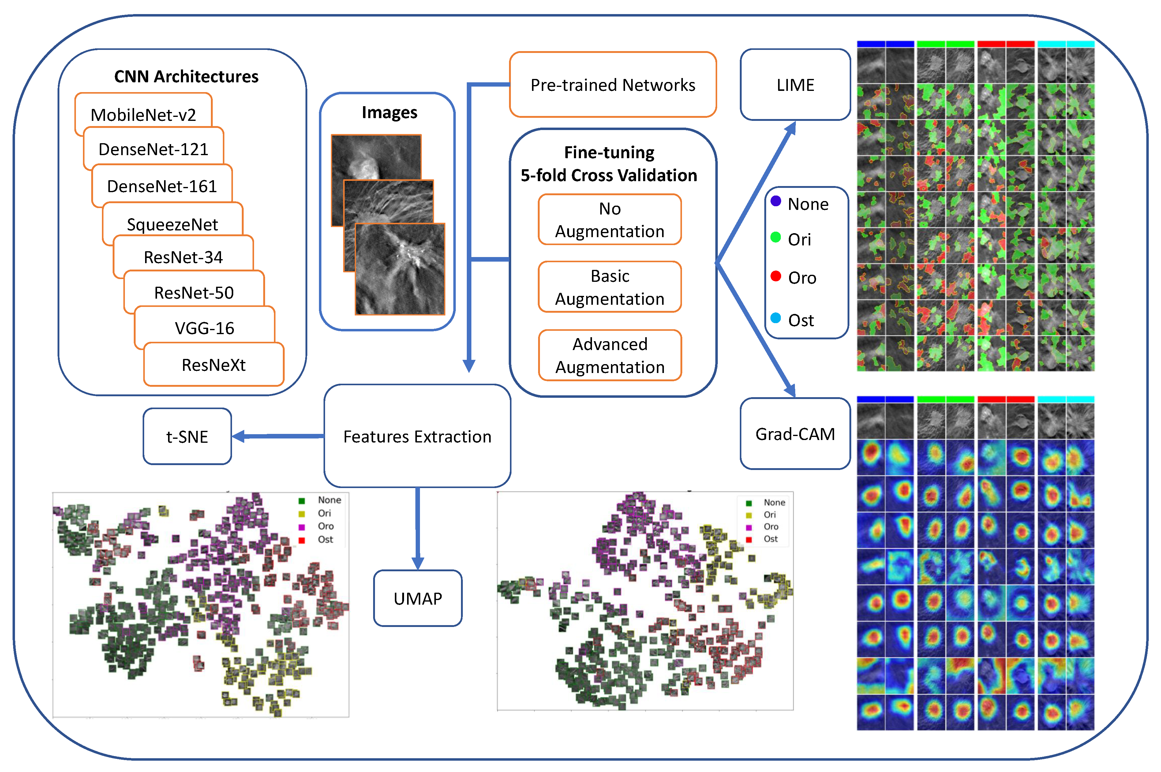
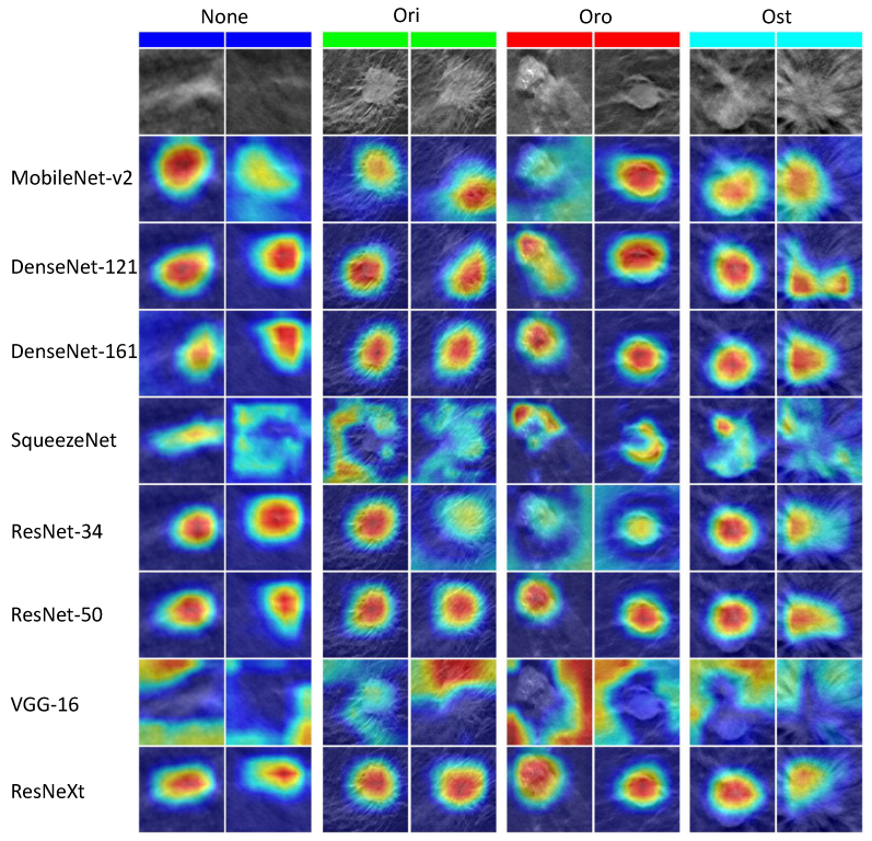
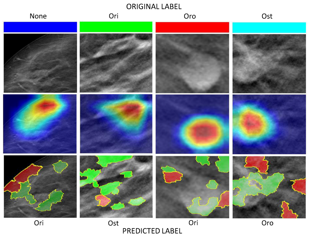
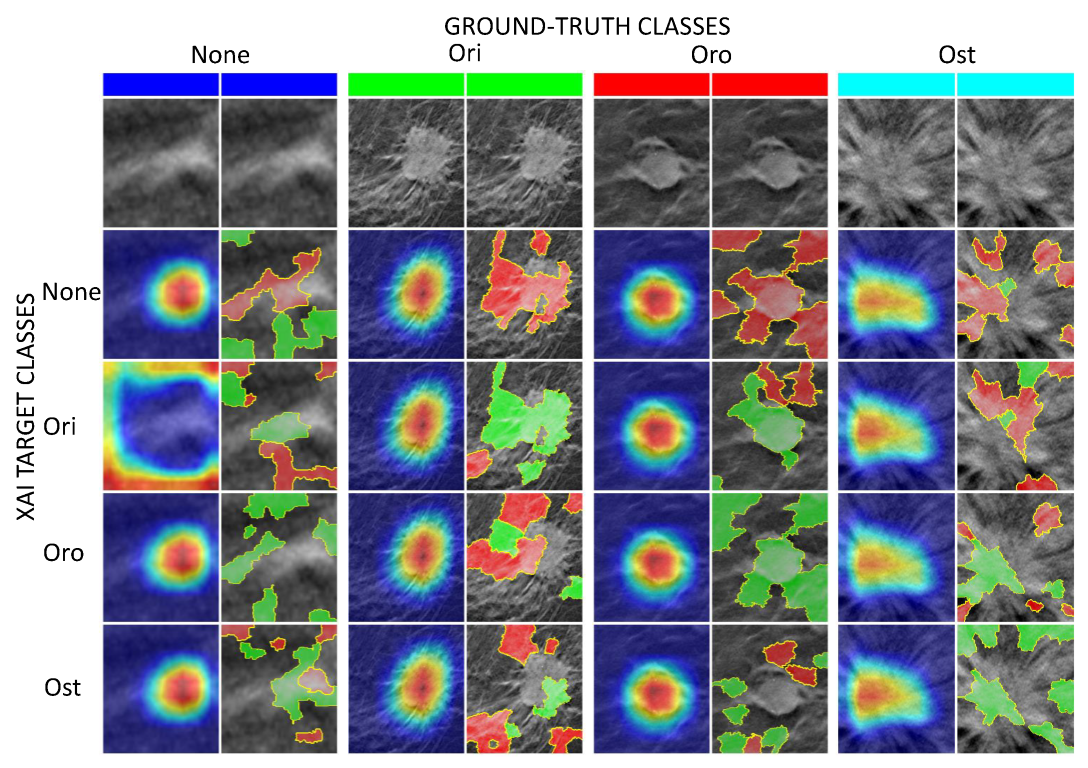
This study adopts two of the most widely admired XAI-based perceptive explanation methods called Grad-CAM and LIME [34] in order to explain the decisions made by the CNN architectures. Both the models are post hoc (i.e., they take as input an already trained model [34]) and can be extended to any DL network for explanation without any alteration in the rudimentary mechanism of the DL methods. Below, a brief description of the Grad-CAM and the LIME models is reported.

• Grad-CAM
  According to Das et al. [55], Grad-CAM can be classified as a back-propagation-based method, meaning that the algorithm makes several forward-passes (one or more) through the neural network and generates attributions during the back-propagation stage using partial derivatives of the activations. Contrary to the CAM, which requires a particular pattern of network under analysis, the Grad-CAM is the generalization that can be applied without any modifications in the DL model [56].
  The Grad-CAM produces a heatmap of the class activation in response to the input image and a class. In other words, for a particular provided class, the Grad-CAM produces approximate and comprehensible representations of the network’s decision-making mechanism in the form of a heatmap that translates to the feature importance. Specifically, in the last layers of a CNN, neurons look for semantic information associated with a specific class. In this layer, Grad-CAM uses the gradient flowing into it to assign a weight to each neuron according to its contribution to the decision in the classification task. The computed information is translated into a jet color scheme to depict the saliency zones, where the red color represents the higher intensity, i.e., pixels on which the network is focusing more for performing the classification, while the blue color represents the lower intensity of the focus.
• Local Interpretable Model-Agnostic Explanations
  In this study, the authors incorporated another well-known explanation technique based on model-agnostic phenomena known as LIME, that can be applied to any DL model. Specifically:

  -

  Local: states that LIME explains the behavior of the model by approximating its local behavior;

  -

  Interpretable: emphasizes the ability of the LIME to provide an output useful to understand the behavior of the model from a human point of view;

  -

  Model-Agnostic: means that LIME is not dependent on the model used; all models are treated as a black-box.

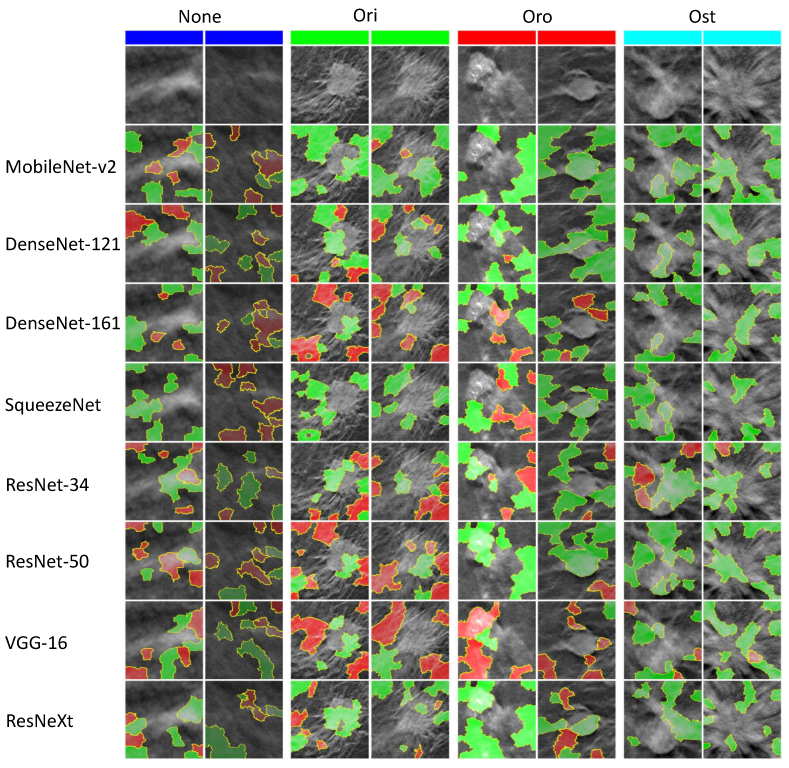
  In our classification problem, the explanation of LIME remains simple. It takes the superpixels (a patch of pixels) of the original input image after generating a linear model, and generates several samples by exploiting the superpixels. The quick-shift algorithm is responsible for the computation of superpixels of an image. Thereafter, the perturbation images are generated and the final prediction is made.
  Afterwards, a heatmap appears over the image that highlights the important pixels, i.e., regions that contribute in classification. The positively contributing features are highlighted in green while the negatively contributing superpixels are colored in red. The LIME also allows to pick a threshold value to select the number of top contributing pixels, either positively or negatively.

3.3.2. Mathematically Explained XAI

This section introduces two widely adopted and useful techniques for performing the task of mathematical interpretability implemented in the presented work. The mathematical interpretability offers t-SNE and UMAP techniques to represent the high-dimensional graph into lower dimensional space without compromising on the clustering structure.

Primarily, both the t-SNE and UMAP are meant for visualization; however, the main difference lies in the interpretation of the distance between the clusters. The t-SNE merely preserves the local structure in the data, whereas the UMAP can preserve both local and global structure in the data, which means that unlike the UMAP, the dissimilarity and the distance between clusters can not be interpreted with the t-SNE.

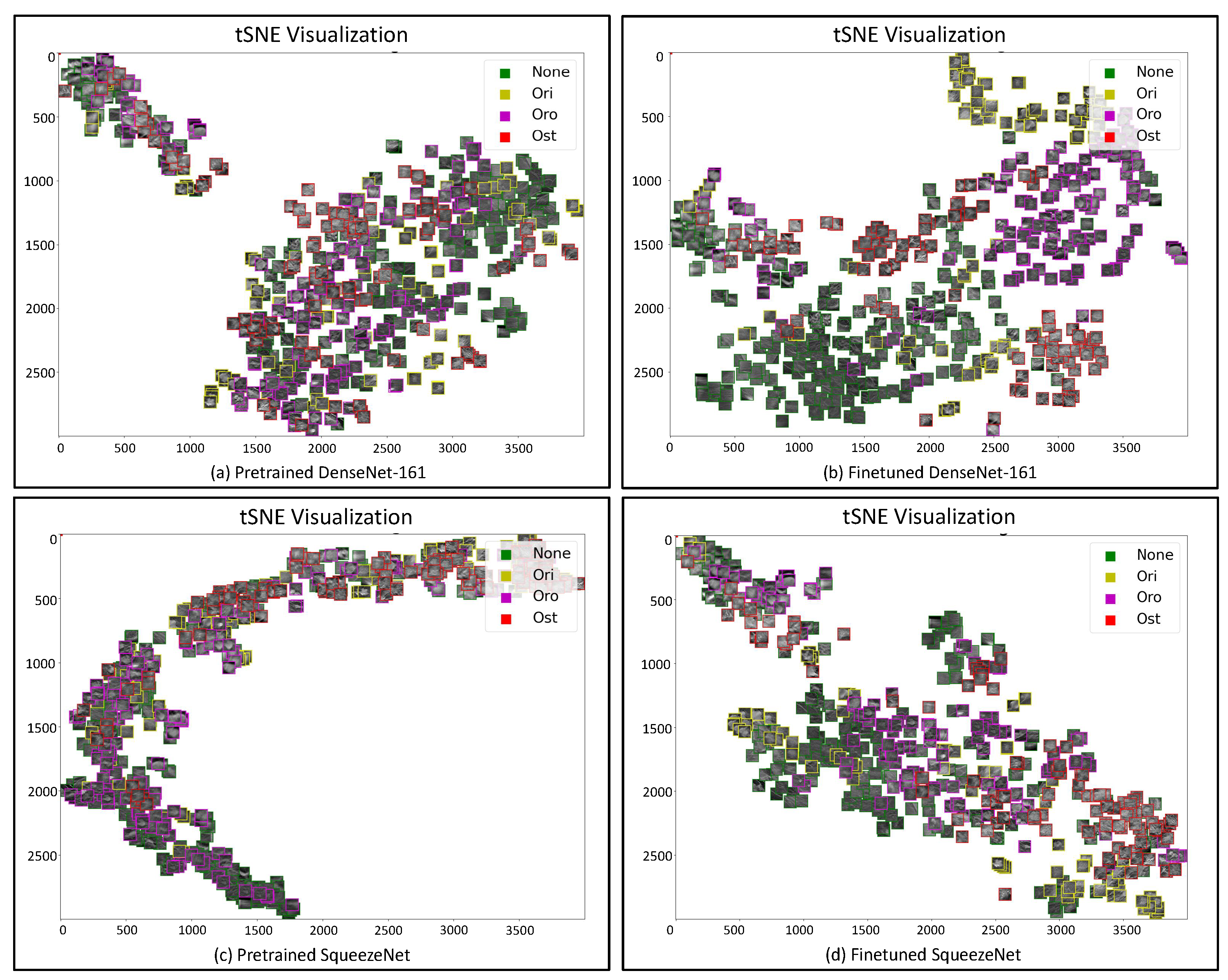
• T-Distributed Stochastic Neighbor Embedding (t-SNE)
  The t-SNE [57] is a variation of the SNE technique that makes the visualization of high-dimensional data possible by associating with each datum a location in lower dimensional space of two or three dimensions. It has been developed to face two issues that affect SNE technique:

  1.

  The optimization of the cost function, by using a variation of SNE cost function (symmetrized) and using a Student’s t distribution for the computation of similarity between two datapoints in the lower-dimensional space.

  2.

  The so-called “crowding problem”, by using a heavy-tailored distribution in low-dimensional space.

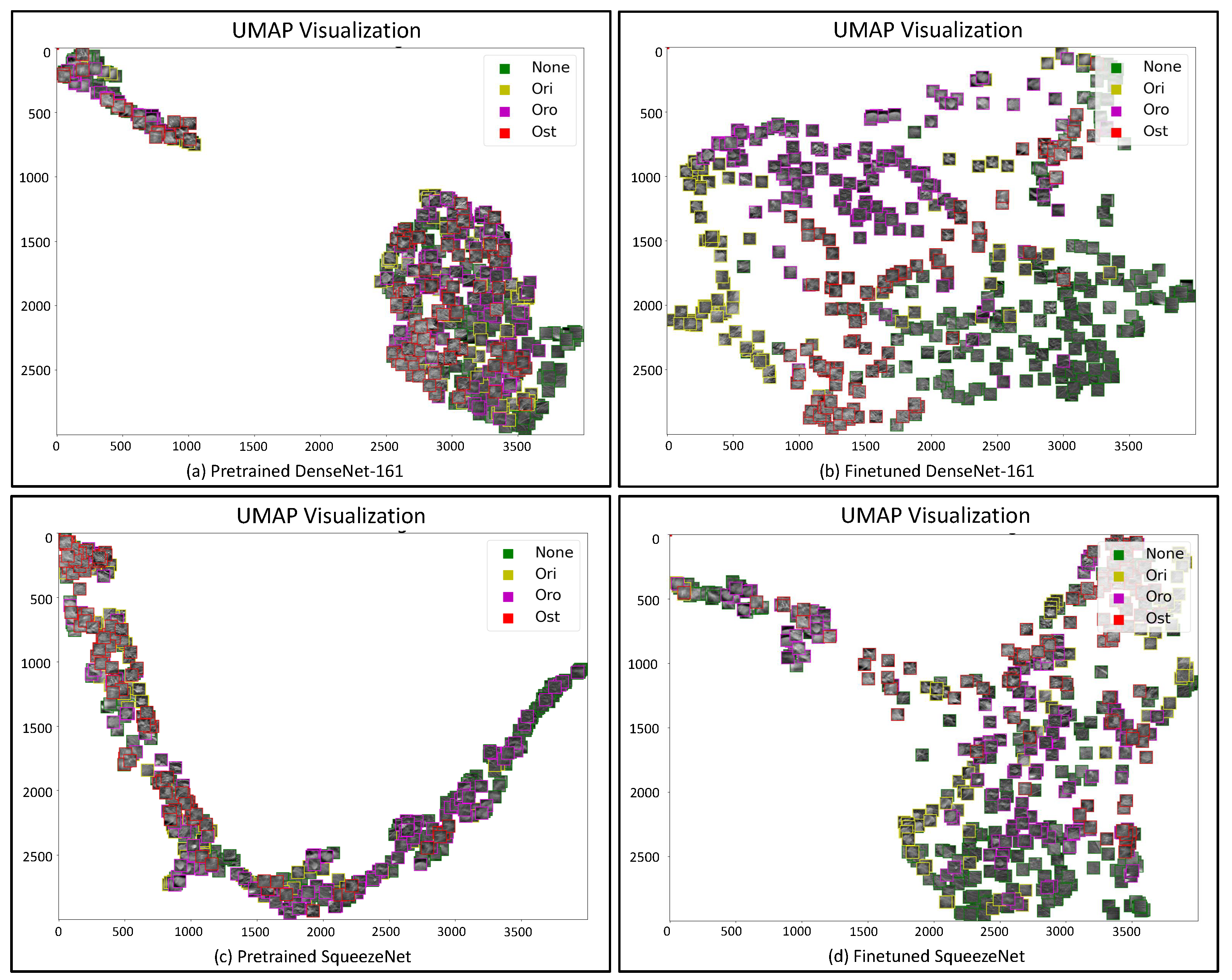
• Uniform Manifold Approximation and Projection (UMAP)
  The UMAP [58] is a nonlinear technique for the dimensionality reduction. It is based on three assumptions:

  1.

  Data are uniformly distributed on an existing manifold;

  2.

  Topological structure of the manifold should be preserved;

  3.

  Manifold is locally connected.

  The UMAP method can be divided into two main phases: learning a manifold structure in a high-dimensional space and finding the relative representation in the low-dimensional space. In the first phase, the initial step is to find the nearest neighbors for all datapoints, using the nearest-neighbor-descent algorithm. Then, UMAP constructs a graph by connecting the neighbors identified previously; it should be noticed that the data are uniformly distributed across the manifold, so the space between datapoints varies according to regions where data are denser or sparse. According to this assumption, it is possible to introduce the concept of ‘edge weights’: from each point, the distance with respect to the nearest neighbors is computed, so the edge weights between datapoints are computed, but there exists a problem of disagreeing edges.

3.4. Experimental Workflow

Figure 5 shows the overall flow diagram of the experimental approach. As depicted, the experimental setup starts by fine-tuning the considered pretrained networks with three different datasets, i.e., the original one and two datasets obtained with two different data augmentation procedures. Thereafter, the features extracted by the features maps of all versions of fine-tuned and pretrained networks were analyzed with both t-SNE and UMAP. Finally, Grad-CAM and LIME were applied to the RoI images.

3.4.1. Data Augmentation Procedures

Due to the unavailability of large datasets, two types of augmentation were considered, i.e., basic and advanced. The basic augmentation comprises rotation and flip, whereas the advanced augmentation also includes color jittering. Numerous configurations with respect to data augmentation were considered, as reported in the

Table 1. Data augmentation summary. All augmentations are carried out on the fly with 0.25 probability in the order they are presented in the table. ’No Aug’, ’Basic Aug’ and ’Adv Aug’ stand for ’No Augmentation’, ’Basic Augmentation’ and ’Advanced Augmentation’. The ✓ and ✗ symbols mean that the transform is included or excluded, respectively. Normalization is always performed at after all other augmentations. ColorJitter refers to the random alterations of the brightness, range: $[0.8,1.2]$; contrast, range: $[0.8,1.2]$; saturation, range: $[0.8,1.2]$; and hue, range: $[-0.2,0.2]$.

Transform	No Aug	Basic Aug	Adv Aug
RandomRotation90	✗	✓	✓
RandomRotation180	✗	✓	✓
RandomRotation270	✗	✓	✓
RandomHorizontalFlip	✗	✓	✓
RandomVerticalFlip	✗	✓	✓
ColorJitter	✗	✗	✓
Normalization	✓	✓	✓

and described hereunder. By exploiting the transforms.Compose interface provided by PyTorch [59], the augmentations are sequentially performed on the fly, each with a given probability that has been set to 0.25.

No Aug refers to the adoption of no augmentation, with the exception of normalization, by rescaling intensity values of images from integers ranging [0, 255] to float values in [0, 1]. Basic Aug consists of performing random rotation by the degrees in multiples of 90, and performing random horizontal and vertical flips. Adv Aug takes advantage of ColorJitter transformations in addition to the previous configuration of basic augmentation. The advanced augmentation comprises random perturbations of brightness, contrast, saturation, and hue. Finally, normalization is performed similar to No Aug.

3.4.2. Training Procedures and Cross-Validation

This study also implements the transfer learning (TL) paradigm using the weights of eight well-known CNN architectures, which not only saves the computational time but also produces higher performance outcomes. The major benefit of using TL comes into practice when the available dataset is not sufficiently large, whereas the performance also remains considerable on small datasets. For the classification problems, applying a pretrained model seems more rational rather than developing a model from scratch. This approach is also referred to as TL because the pretrained models’ weights are transferred to other models to address the similar image classification problems.

Moreover, since the manual tuning of parameters is a time-consuming and less efficient process, this study encompasses the grid search to initially select, but later on settles to the learning rate of $1\times {10}^{-5}$, batch size of 32, and number of epochs to 50. Furthermore, a range of optimizers is available which can be selected depending upon the nature of problem; however, in this work, the Adam optimizer is used due to the simplicity and effectiveness on the classification problems. The used loss function was the cross entropy. Additionally, moving towards the train–test split, 5-fold cross-validation with stratification is performed in such a manner that approximately 80% of the data belonging to each class resides in train partition, whereas the remaining 20% dwells in the validation set.

3.5. Classification Performance Assessment

The results of all pretrained and fine-tuned nets are analyzed based on area under the curve (AUC). The mean and standard deviation of AUC are computed for each classifier among 5-fold results. The AUC and the standard deviation are also computed for each individual class against all architectures in three augmentation configurations.

Furthermore, the training and validation losses during the experimental procedure are also plotted to investigate the eventual problems that arise during the potential overfitting at each epoch. All the experiments are performed on a machine running on Windows 10 operating system, and a Python 3.7 environment is exploited with PyTorch (torch v1.10.0, torchvision v0.11.0), grad-cam v1.3.6, and lime v0.2.0 libraries for DL and XAI. To this end, CUDA 11.3 is used to take advantage of the GPU power.

Explainable AI

Lastly, the saliency maps using Grad-CAM algorithm are analyzed, and superpixel importance (both positive and negative) with the LIME technique is used to inquire what aspects the classifiers are focusing on, so as to build a trust for CAD systems that can be exploited to support the radiologists’ diagnostic workflow are computed. Generally, these methods identify which features oblige a DL model to discriminate among different lesions present on the image.

Particularly, to generate the heatmap visualizations from the Grad-CAM, all the architectures, except the VGG-16, utilize the last layer before the global average pooling layer. In case of VGG-16 architecture, the Grad-CAM is run at the maxpool layer before the first fully connected layer. Note that VGG16 is the only CNN among the considered architectures in this study that does not implement global average pooling, since it is an old architecture based on stack of fully connected layers at the end. On the other hand, the LIME is a model-agnostic method; therefore, it creates the perturbations once the CNN finishes the classification task. In both cases, the specific class modeled as base class differs for all the networks; therefore, the labeled and the targeted classes are provided within figures. Moreover, the t-SNE and UMAP embeddings, before and after the fine-tuning of all architectures on the DBT image training set, are computed to understand how well TL approaches work on the radiological image scenario. The feature sets considered for t-SNE and UMAP are the same as for Grad-CAM discussed above.

4. Experimental Outcomes

The section below illustrates the experimental results of the study in terms of the classification performance, XAI outcomes, and the relevant training and validation trends. The section contains a comparative analysis of the employed techniques and highlights the identified significant trade-offs.

4.1. Performance Module

The summary of the experimental results of all eight CNN models considered in this study in terms of AUC with 5-fold cross-validation is provided in

Table 2. The summary of the results obtained for No Aug, Basic Aug, and Adv Aug configurations is provided hereunder. The bold text represents the best value of the corresponding parameter among all CNN models, which is mean over all four classes.

Architecture	Area under the Curve (AUC)
	No Aug (None, Ori, Oro, Ost)	Basic Aug (None, Ori, Oro, Ost)	Adv Aug (None, Ori, Oro, Ost)
MobileNet-v2	91.9 ± 1.1	92.4 ± 0.9	93.6 ± 1.2
	97.4 ± 0.4	98.0 ± 0.6	97.6 ± 0.9
	95.2 ± 1.3	95.9 ± 1.1	96.3 ± 0.9
	95.8 ± 0.7	96.6 ± 0.5	96.5 ± 0.7
	95.1	95.7	96.0
DenseNet-121	90.1 ± 1.2	93.9 ± 1.9	94.5 ± 1.3
	94.2 ± 1.4	98.5 ± 0.6	98.2 ± 0.8
	89.9 ± 1.7	95.5 ± 0.6	96.7 ± 0.8
	92.9 ± 1.8	97.1 ± 0.8	97.2 ± 1.2
	91.8	96.2	96.6
DenseNet-161	94.8 ± 0.9	95.8 ± 1.0	96.4 ± 0.5
	97.6 ± 1.4	99.1 ± 0.7	99.4 ± 0.2
	95.8 ± 1.3	97.8 ± 1.0	98.7 ± 0.7
	97.0 ± 0.9	98.2 ± 0.3	98.0 ± 0.7
	96.3	97.7	98.2
SqueezeNet	50.9 ± 3.0	56.6 ± 5.6	62.7 ± 8.1
	85.9 ± 3.2	84.3 ± 1.4	86.4 ± 2.9
	68.9 ± 5.6	67.6 ± 3.8	71.7 ± 7.2
	83.8 ± 2.6	86.2 ± 3.7	87.6 ± 3.1
	72.4	73.7	77.1
ResNet-34	92.0 ± 0.8	94.5 ± 1.0	95.4 ± 0.6
	96.2 ± 0.8	98.6 ± 0.5	98.9 ± 0.5
	94.7 ± 1.7	97.6 ± 0.4	97.4 ± 1.0
	96.1 ± 1.3	97.6 ± 0.7	97.7 ± 0.7
	94.8	97.1	97.3
ResNet-50	93.8 ± 1.1	95.3 ± 1.2	96.2 ± 0.6
	98.0 ± 0.5	99.4 ± 0.3	99.3 ± 0.3
	95.8 ± 0.8	97.8 ± 0.6	97.9 ± 0.7
	97.0 ± 1.0	97.8 ± 0.9	98.5 ± 0.4
	96.1	97.6	98.0
VGG-16	90.6 ± 1.7	92.5 ± 1.4	93.6 ± 1.3
	98.1 ± 0.6	98.9 ± 0.6	97.7 ± 0.7
	96.1 ± 0.7	96.7 ± 0.7	97.2 ± 0.7
	96.6 ± 0.4	97.7 ± 0.6	98.1 ± 0.6
	95.3	96.4	96.6
ResNeXt	94.1 ± 1.0	96.1 ± 0.7	95.8 ± 0.7
	97.7 ± 0.7	99.3 ± 0.2	99.0 ± 0.7
	96.0 ± 0.8	97.9 ± 0.7	98.2 ± 0.8
	97.1 ± 0.5	98.3 ± 0.3	98.2 ± 0.9
	96.2	97.9	97.8

for the three conceived experimental configurations, i.e., without augmentation (No Aug), with basic augmentation (Basic Aug), and with advanced augmentation (Adv Aug), respectively.

4.1.1. Classification Results

In the case of No Aug configuration, it can be observed from Table 2 that DenseNet-161 is the architecture with the highest mean AUC of 96.3%. The ResNeXt and ResNet-50 networks are slightly behind, with AUC of 96.2% and 96.1%, respectively. The MobileNet-v2, ResNet-34, and VGG-16 collectively form a third cluster with AUC of around 95%. Conversely, the SqueezeNet is the worst-performing model in our experimental setup, managing to achieve merely 72.4% AUC.

In the case of the Basic Aug configuration, all architectures performed considerably better than the previous No Aug configuration. The results reveal that ResNeXt obtained the highest AUC of 97.9%, beating all other architectures. The DenseNet-161 and ResNet-50 achieved similar performances with the AUC of 97.7% and 97.6%, respectively. Once again, the performance of the SqueezeNet failed to present significant outcomes, thus abiding by the No Aug configuration.

The second augmentation setup, called Adv Aug, emerged to be even better than both previously conceived No Aug and Basic Aug setups. The DenseNet-161 reached the top AUC of 98.2%. The ResNet-50 appeared to be the second best model, with a slightly lower AUC of 98.0%.

Finally, as noted during the No Aug and Basic Aug configurations, the SqueezeNet is the model which offers least reliability with the largest inter-fold variability; however, it improved the AUC from the previous setups.

Therefore, it can be summed up that the ResNeXt and DenseNet-161 remain the top-performing models, and the augmentation configurations considerably improved the performance of all CNN architectures. However, the SqueezeNet failed to produce convincing results.

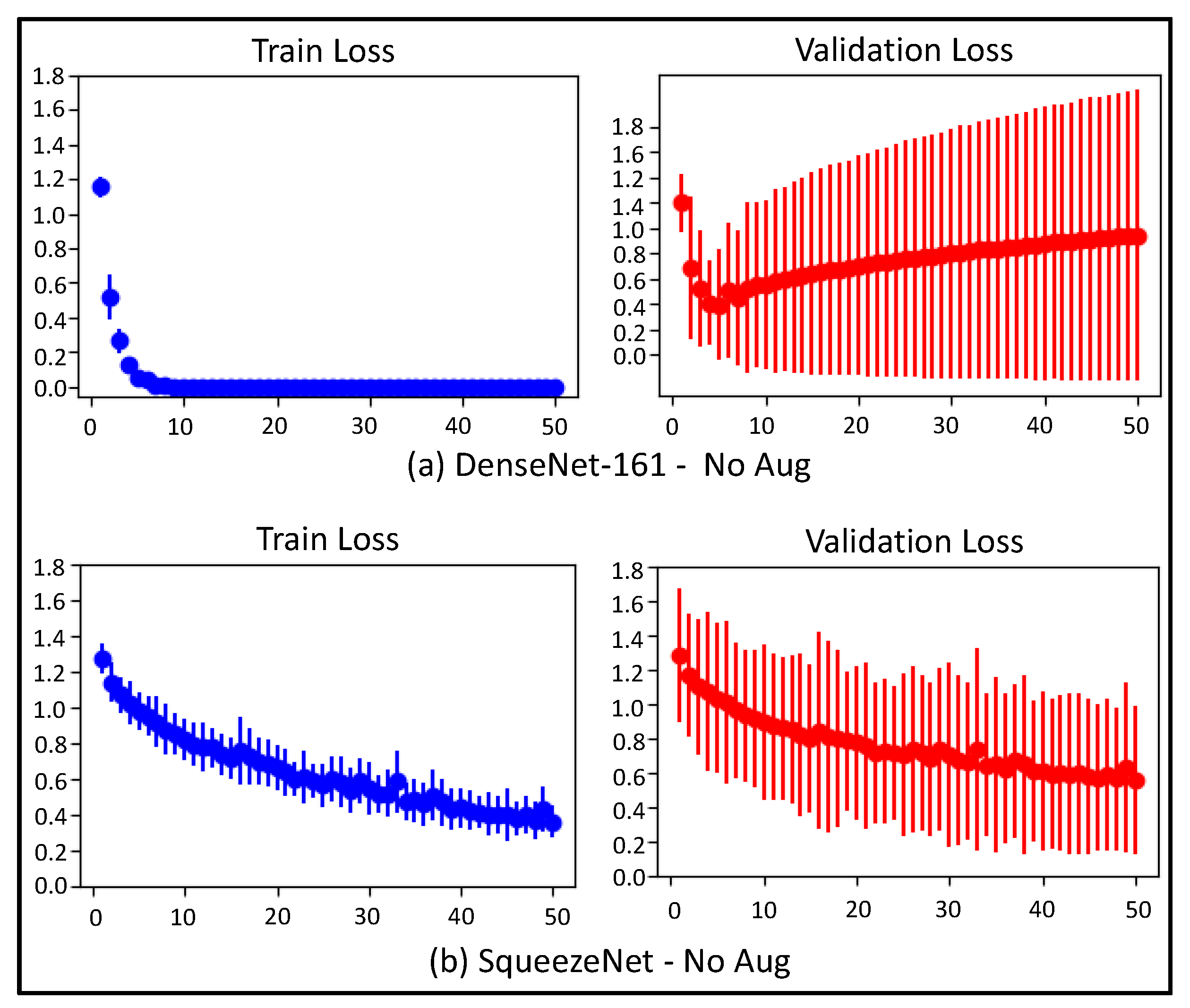
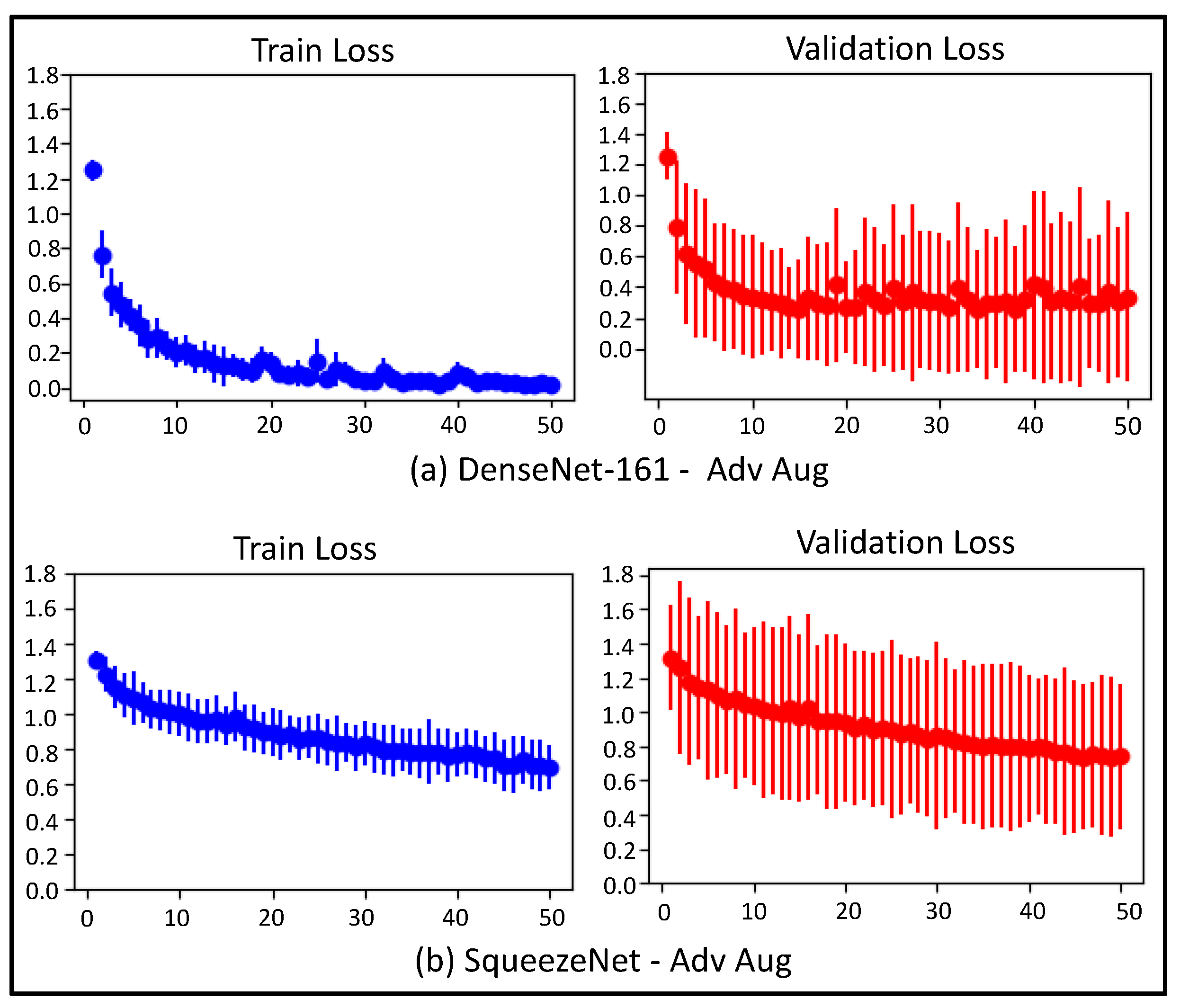
4.1.2. Train and Validation Loss Trends

The training and validation losses fluctuate with respect to each epoch. All models were run at different values of epoch starting from 10 up to 50; however, for the purpose of clarity and concision, only the results obtained considering the 50 epochs are illustrated.

The loss curves demonstrate important trends to monitor in order to clearly distinguish the working mechanism of the CNN architectures over the repeated iterations. In Figure 6, it is distinctive to visualize the loss on both train and validation sets (first fold) for the best, i.e., DenseNet-161, and the worst, i.e., SqueezeNet, CNN architectures in the case of No Aug configuration.

Although the SqueezeNet shows decreasing loss on both train and validation sets in Figure 6b, the training loss curve becomes constant right after fewer epochs in DenseNet-161 in Figure 6a. Moreover, the validation curve depicts increasing behavior after fewer than ten epochs for the DenseNet-161. Such behavior could be motivated by the huge number of parameters that might cause the overfitting problem on the train set.

The train and validation loss curves considering the advanced data augmentation configuration are provided in Figure 7. The augmentation helped the DenseNet-161 to overcome the increasing validation loss, as shown in Figure 7a. This evidences that incorporating on-the-fly data augmentation solved the overfitting issues. However, the SqueezeNet struggles to keep the loss low, as depicted in Figure 7b, and ends up with even worse performance than the no augmentation configuration. Differently from DenseNet-161, the SqueezeNet does not seem to take advantage of the on-the-fly augmentation, possibly due to lower number of parameters.

Additionally, the reported behavior of the loss trends on both train and validation sets is comparable to the other folds. With the intention of concision, authors decided to depict the outcomes of the best and the worst performing architectures, i.e., DenseNet-161 and SqueezeNet, respectively, in terms of AUC and loss.

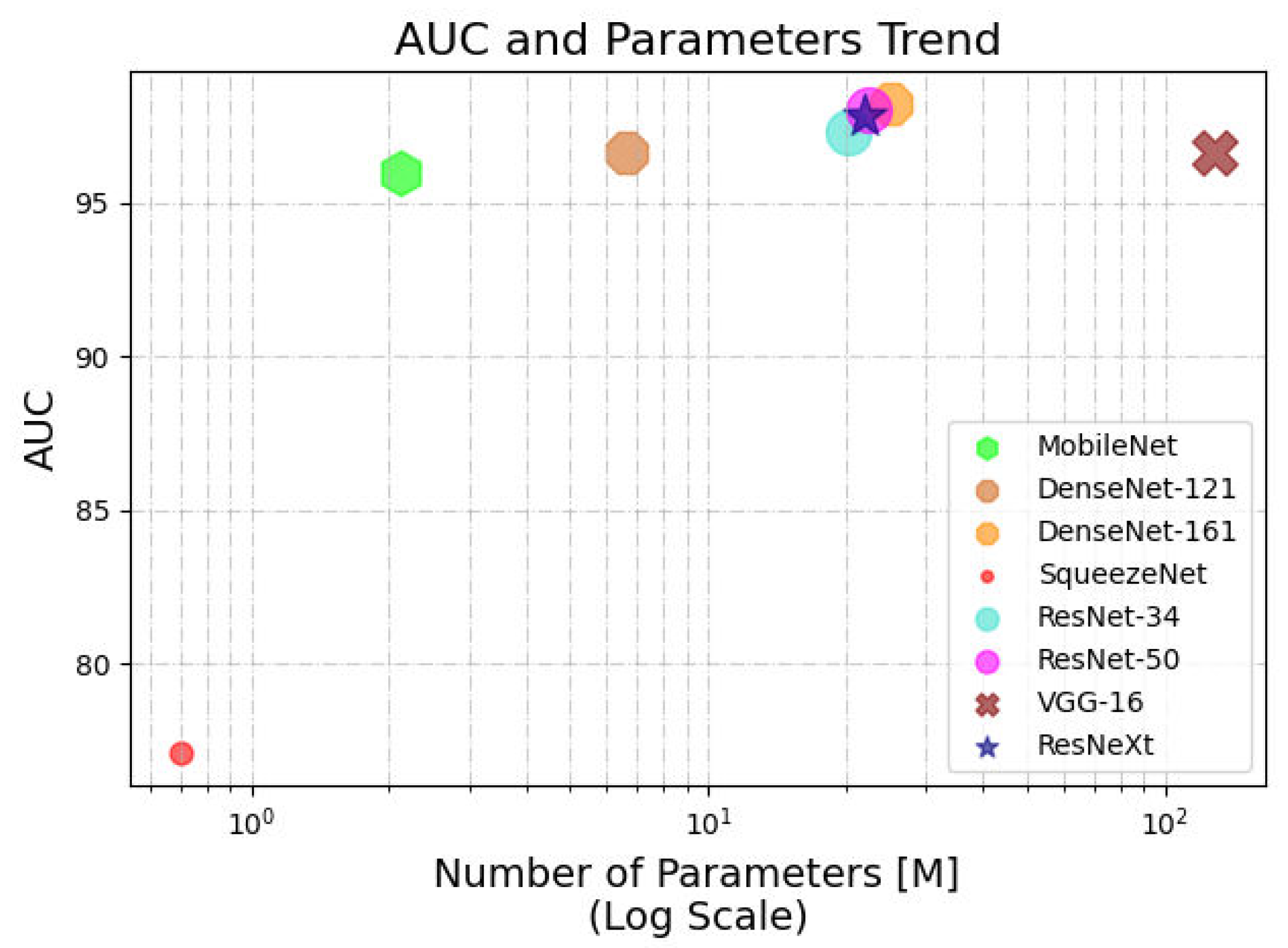
4.2. Area under the Curve and Number of Parameters Trade-Off

During the experimental phase, the authors came across an interesting trend between the mean AUC (computed on the test set) and the number of parameters of the employed architectures. A plot illustrating the relationship between AUC and the number of parameters for the eight considered CNNs is presented in Figure 8. It is observable that the VGG-16 holds a gigantic number of parameters but without yielding the corresponding improvement in the AUC. The SqueezeNet, on the contrary, is a small architecture in terms of number of parameters, but fails to realize commendable AUC among the contemplated models. The best trade-off between the number of parameters and the performance can be seen in ResNet-like models, with ResNet-50 winning the dispute.

4.3. XAI Interpretation

This study employed XAI techniques from two families comprising mathematical interpretability, i.e., t-SNE and UMAP, and perceptive interpretability, i.e., Grad-CAM and LIME. The experimental outcomes of both XAI approaches on all CNN models are explained hereunder.

4.3.1. t-SNE and UMAP

The extracted features from both pretrained and fine-tuned networks are visualized in order to understand what patterns emerge in low-dimensional spaces after having employed nonlinear dimensionality reduction techniques such as t-SNE and UMAP.

In Figure 9, the t-SNE embedding plots for both pretrained and fine-tuned DenseNet-161 and SqueezeNet architectures are pictorially represented. Similarly, Figure 10 presents the UMAP embedding plots for both pretrained and fine-tuned DenseNet-161 and SqueezeNet models. In the pretrained version, no clear patterns arise from both embedding plots, showing that features learned from ImageNet dataset are not necessarily well discriminative for radiological image applications.

Nonetheless, after 50 epochs of fine-tuning on the designated train set, the clusters appear more distinctive. In fact, with trained CNN features, both UMAP and t-SNE allow to visualize different clusters for all four considered classes: None, Ori, Oro, and Ost.

As described in Section 3, the distance between the clusters cannot be interpreted by using the t-SNE visualizations. For instance, it cannot be inferred from Figure 9 that clusters are dissimilar to each other when one cluster is closer to the other. However, it can be stated that points closer to each other are more similar objects than the points at farther ends, whereas Figure 10, thanks to the local and global feature representation capability of the UMAP, clearly plots the points that can be interpreted as distinguishing clusters and the position of the points.

4.3.2. Class Activation Mapping

The visual explanation of all eight fine-tuned networks is pictorially depicted in Figure 11, considering the Grad-CAM as reference method. In the figure, two sample images for every class are depicted, and the corresponding saliency maps are reported for every network. This figure considers only images for which every network makes the correct prediction, in order to visualize the link between the highlighting of the lesion area and the network performance. The saliency maps of the approximate features are generated considering the ground truth/predicted class view.

Interestingly, the CNN architectures that find troubles in correctly identifying the lesion areas also appear to have worse performance in the classification task. For instance, SqueezeNet, which is the worst-performing network in terms of AUC, and VGG-16, which also appears to have a trade-off between AUC and the number of parameters, as shown in Figure 8, fail to spotlight the relevant lesion area. Here, the trade-off refers to the fact that the increasing number of parameters seldom yields increased AUC. In contrast, DenseNet-161, DenseNet-121, and ResNet-50 correctly highlight the lesion on the images. Thus, our XAI-based CAD system unveils the potential applicability of the reliable and suspicious candidates to adopt in the CAD systems.

4.3.3. Local Interpretable Model-Agnostic Explanations

It is worth mentioning that the visual results of the Grad-CAM and LIME must not be confused. Unlike the Grad-CAM method, which emphasizes the lesion area with the intensity of the color closer to the center, the LIME method works differently by providing the top contributing s that resulted in the classification of the image into any given class. However, in both cases, the images were generated by observing the ground truth/predicted class view.

The s perturbations performed by the LIME are shown in Figure 12. The observations experienced with respect to the performance of the LIME technique are similar to the Grad-CAM method. The figure reports the exact images that were compared in Figure 11 for the Grad-CAM method, to create a robust and clear comparison. The class considered for performing the LIME perturbations is the ground truth class, which, in this case, corresponds also to the prediction of all the CNNs. The regions which are positively correlated with the decision made by the CNN are highlighted in green, whereas those negatively correlated are colored red.

However, it has to be noted that reasoning in terms of s can result in explanations which are visually less clear to understand than those of their CAM-based counterpart. Comparing Figure 11 and Figure 12, we can see that some superpixels which are correlated to the prediction according to the LIME method are not considered relevant in the corresponding Grad-CAM activation maps. Therefore, we advise to consider both methods when trying to devise an explanation for a CAD system, in a way that complementary information can be extracted from both sources to obtain a broader view of how the model is working.

5. Discussion

This study proposes a novel, visually explainable DL-driven multiclass shape-based breast cancer classification framework for tomosynthesis lesion images. For the task of morphological classification, eight DL models are employed on tomosynthesis breast images and two families of XAI methods, i.e., perceptive interpretability and mathematical interpretability, are incorporated to explain the results acquired during the validation study in order to create the trust among the clinicians and AI.

The perceptive interpretability models are responsible for visually explaining the top contributing features towards the classification, whereas the mathematical interpretability methods portray feature clustering capabilities of the DL architectures. The CAD system developed in this study is able to encircle the potential growth pattern of the tumorous regions on the DBT images and results in the improved diagnostic and prognostic performance. The successful implementation also enhances the trustworthiness among the clinical field and the high-accuracy-yielding DL architectures.

The sections below comparatively discuss the shape-based breast cancer classification and the interpretation of the DL models using XAI techniques.

5.1. Shape-Based Breast Cancer Classification

Quantitatively, the extensive experimental results are elaborated, considering the pretrained DL methods on both with and without data augmentation configurations. The mean AUC values of the developed models improved during the augmentation phases. The crown of overall best performing algorithm belongs to DenseNet-161 due to persistent performance, i.e., reaching higher than 96.0% across No Aug, Basic Aug, and Adv Aug setups.

In particular, the best-performing model, i.e., DenseNet-161, increases by 1.45% and 1.97% in the mean AUC from No Aug to Basic Aug and Adv Aug, respectively. It impressively increases by 33.01%, 33.28%, and 27.10% over the SqueezeNet in configuration-to-configuration comparison, i.e., No Aug to No Aug, and so on. In the case of Basic Aug, the ResNeXt outperforms all other architectures with a percent increase of 33.56 from the worst-performing model.

Since the results are comparable, any particular model performing best in terms of AUC and loss may not perform ideally in all aspects. The reason is the primitive learning and weight updating mechanism of the CNN models. For example, in the No Aug phase, three out of four individual AUC values of ResNeXt among classes remain higher than the respective individual AUC values of the DenseNet-161, despite the equal mean AUC.

The utilization of the augmentation techniques revamped the trends of the validation loss, as shown in Figure 6 and Figure 7; however, the improvement in the validation loss is negative for the worst-performing model, i.e., SqueezeNet, which fluctuates between 0.3 to 1.3 and 0.7 to 1.3 for No Aug and Adv Aug configurations, respectively. Both the training and validation losses increased.

The illustrated loss values are evidently coherent to the fact that a huge model such as DenseNet-161, with tons of parameters, overfits when it is trained with no augmentation over an increasing number of epochs in our experimental setup. Instead, SqueezeNet has the opposite problem, being unable to even properly comprehend the fundamental patterns, resulting in an underfit behavior. After augmentation, underfitting problem of SqueezeNet cannot be resolved, as shown by comparing Figure 6b and Figure 7b, but the overfitting issue of the DenseNet-161 is mitigated as presented by comparing Figure 6a and Figure 7a.

A noteworthy consideration arises when considering the performance of a model in relation to its size and complexity. In Figure 8, a noteworthy trend exists between the number of parameters and the AUC, the models having a huge number of parameters compromised at the mean AUC at certain levels. On the contrary, the models with an extremely low number of parameters may result in bad generalization performance, since with reduced number of parameters, the model is hardly able to learn simple patterns in our study.

Nevertheless, the two different augmentation configurations and three different execution setups (i.e., 10, 30, and 50 epochs) disclose a clear improvement with augmentation in our DBT classification framework. The basic augmentation improves performance compared to no augmentation, and the advanced augmentation plays its part and further increases the AUC outcomes. One major reason reckoned is the considerably high visually noticeable resemblance between the training and the validation data, whereas the state-of-the-art architectures, the significant clinical data, and the RoI-level cropped images may possibly be other driving causes.

5.2. Explainable AI in Breast Cancer Classification

Concerning the mathematical explanation, as emerged from the visualization of the feature embeddings, one can discern that both t-SNE and UMAP are able to extract meaningful relationship in the low-dimensionality spaces when the features are representative of the underlying patterns in the sample images. In Figure 9 and Figure 10, four clusters are clearly visible for the DenseNet-161 architecture. On the contrary, when the model is less accurate, as in the case of fast and light SqueezeNet (in terms of number of parameters), the cluster formation behaves differently, with UMAP resulting in more compact representations. As a general suggestion, therefore, the study recommends to use these mathematical XAI techniques to visualize if considered features for a problem under consideration are relevant.

With respect to the perceptive XAI techniques, the performance results of the CNN models are aligned with the complementary information that can be extracted from Grad-CAM and LIME methods. While the first allows to detect which regions have a gradient that is deemed relevant for performing the prediction, the second permits to understand, for each superpixel, if it is positively or negatively correlated to the prediction. Moreover, the LIME method has an adjustable parameter for deciding the number of top contributing features to show over the original image. Since we already have the intensity values from the saliency maps of Grad-CAM, we decided to mark in green every positively correlated region and in red every negatively correlated region, so that the mixed information obtained can be exploited to obtain an intuitive understanding of which regions are more important (higher intensity values in CAM maps), and which are positively or negatively correlated to the final outcome (green and red, respectively).

Interestingly, the CNN architectures that find trouble in correctly identifying the lesion areas also appear to have a lower AUC. Thus, on a general scale, the higher AUC can be explained by using XAI methods. For instance, the SqueezeNet, which is the worst-performing network in terms of AUC and validation loss, and VGG-16, which has a trade-off between the AUC and the number of parameters, as shown in Figure 8, fail to spotlight the relevant lesions as illustrated in Figure 11. In contrast, DenseNet-161, DenseNet-121, ResNeXt, and ResNet-50, which feature higher AUC values, correctly highlight the lesion when tested with the Grad-CAM method.

Moreover, as the loss trends and the AUC tables show, none of the CNNs yielded 100% performance, which means the misclassified examples are also present. These samples of the misclassified images are also presented to the XAI methods in order to dive into the features that resulted in misclassification. The reason behind misclassification of one type of cancerous image to another type might be related to the homogeneity of the shapes of a few examples with other classes. Figure 13 illustrates the results of both Grad-CAM and LIME methods regarding examples of misclassified images.

The labels provided above the samples represent the ground truth, whereas the labels provided under the saliency maps are the predictions made by the CNNs. This figure proves that XAI could also help the physician understand why the AI is failing. For instance, the None image in the Figure 13 contains a mesh that is not lesion according to the expert radiologists. However, it fools the CNN to misclassify the image as Ori. Both the CAM and LIME methods highlighted the regions that carry analogous properties, thus explaining the cause of the misclassification. It is worth noting that a similar discussion emerges from the other examples provided in Figure 13.

In order to understand how the results of two XAI perceptive methods vary according to the different target classes, Figure 14 reports the explanation results of both methods considering eight different correctly classified images. It is worth noting that the CAM results did not differ among the four XAI target classes. Interestingly, the results are different when LIME is analyzed. For instance, when considering None as target class and visualizing its explanation outcome on an Ori class image, the LIME-highlighted lesion area has a region that contributes negatively towards the classification of the chosen target class. In the same image, the LIME explanation with the Ori target class highlighted the lesion region as green (positively correlated) since the image belongs to the Ori class. This kind of comment could also be easily applied to other images of Figure 14, thus confirming the difference and the utility of more than one perceptive XAI method.

Finally, from several discussed dimensions, our study proves the applicability of the CNN models in the classification task of DBT lesions on RoI level. Taking the advantage of TL, our framework reaches efficient results with fine-tuning of several parameters. The black-box nature of the DL models is successfully unveiled to build the trust of radiologists to emerge towards the reliable CAD systems for the diagnostic tasks.

6. Limitations and Future Directions

In this article, the pretrained DL models are employed for the classification tasks using a 5-fold cross-validation strategy. Since the train and validation data come from the same source, few models suffer from generalizability and overfitting problems. The models can be validated on the external datasets after training for better understanding. Additionally, the dataset used in the study is relatively small; this is a major reason to incorporate the pretrained models and perform fine-tuning also with data augmentation. The used models could be trained and tested with large-scale datasets acquired from different cohorts.

The study also unleashes the hidden classification mechanism of DL techniques by integrating numerous XAI techniques. The Grad-CAM methods produce a coarse localization map. In the experimental outcome section, it can clearly be observed that at a certain point the XAI methods explain the DL methods’ results with slightly different regions. This is because of the model overfitting. A robust investigation may demonstrate productive conclusions. The CAM method only focuses on a general region of the image instead of focusing on minute peculiarities, such as that LIME technique generates the perturbations and highlights the top features. Similarly, the SHapley Additive exPlanations (SHAP) model quantifies the exact amount of contribution made by a particular region, and can be added in future studies.

7. Conclusions

Breast cancer is the leading deadly ailment in women, and its inevitable progression has become a major concern for the healthcare industry. However, timely diagnosis can significantly improve the medication and prevent the further expansion of the cancerous regions. DL offers great success in automatic detection and classification using medical imaging data. However, the black-box nature of the decision-making mechanism of the DL architectures hampers the trust among the clinicians. The XAI techniques uncover the black-box and hidden nature of the DL and provide useful apprehension of the high-accuracy-yielding DL models. This builds confidence in machine learning in the clinical domain and paves the way towards DL-centered image-guided CAD systems.

In this work, authors proposed a robust visually and mathematically explainable DL framework for multiclass shape classification of tomosynthesis breast lesion using eight pretrained CNN models using an in-house dataset. Due to small-scale data availability, the data augmentation was incorporated. The best fine-tuned model achieved mean AUC values of 98.2% and 96.3% with and without considering the data augmentation, respectively.

Furthermore, considering the hypersensitive clinical realm, two families of XAI methods, i.e., perceptive interpretability and mathematical interpretability, were incorporated to visually explain the CNN models’ classification performance. The former interpretability method includes Grad-CAM and LIME, which are responsible for visually explaining the experimental outcomes in terms of feature-level contribution towards classification, whereas the latter method comprises t-SNE and UMAP techniques that portray feature clustering capabilities of the DL architectures. The performances of all models were aligned with the visual and mathematical interpretations, hence developing the necessary trust between the healthcare industry and the DL architectures. The results proved the usability of XAI to understand the mechanism of employed AI models, also in the cases of failures.

In future, authors aim to further enhance the interpretability of the CNN models by calculating the single feature-level weightage towards classification. The authors also plan to investigate the performance of the proposed framework on unforeseen datasets and to integrate the novel DL models.

References

1. Bray, F.; Ferlay, J.; Soerjomataram, I.; Siegel, R.L.; Torre, L.A.; Jemal, A. Cancer statistics 2018: GLOBOCAN estimates of incidence and mortality worldwide for 36 cancers in 185 countries. CA Cancer J. Clin. 2018, 68, 394–424. [Google Scholar] [CrossRef] [PubMed] [Green Version]
2. Esmaeili, M.; Ayyoubzadeh, S.M.; Javanmard, Z.; Kalhori, S.R.N. A systematic review of decision aids for mammography screening: Focus on outcomes and characteristics. Int. J. Med. Inform. 2021, 149, 104406. [Google Scholar] [CrossRef] [PubMed]
3. Rezaei, Z. A review on image-based approaches for breast cancer detection, segmentation, and classification. Expert Syst. Appl. 2021, 182, 115204. [Google Scholar] [CrossRef]
4. Kulkarni, S.; Freitas, V.; Muradali, D. Digital breast tomosynthesis: Potential benefits in routine clinical practice. Can. Assoc. Radiol. J. 2022, 73, 107–120. [Google Scholar] [CrossRef] [PubMed]
5. Wu, M.; Ma, J. Association between imaging characteristics and different molecular subtypes of breast cancer. Acad. Radiol. 2017, 24, 426–434. [Google Scholar] [CrossRef]
6. Cai, S.Q.; Yan, J.X.; Chen, Q.S.; Huang, M.L.; Cai, D.L. Significance and application of digital breast tomosynthesis for the BI-RADS classification of breast cancer. Asian Pac. J. Cancer Prev. 2015, 16, 4109–4114. [Google Scholar] [CrossRef] [PubMed] [Green Version]
7. Sickles, E.; D’Orsi, C.; Bassett, L. ACR BI-RADS® Mammography. In ACR BI-RADS® Atlas, Breast Imaging Reporting and Data System; American College of Radiology: Reston, VA, USA, 2013. [Google Scholar]
8. Lee, S.H.; Chang, J.M.; Shin, S.U.; Chu, A.J.; Yi, A.; Cho, N.; Moon, W.K. Imaging features of breast cancers on digital breast tomosynthesis according to molecular subtype: Association with breast cancer detection. Br. J. Radiol. 2017, 90, 20170470. [Google Scholar] [CrossRef] [PubMed]
9. Cai, S.; Yao, M.; Cai, D.; Yan, J.; Huang, M.; Yan, L.; Huang, H. Association between digital breast tomosynthesis and molecular subtypes of breast cancer. Oncol. Lett. 2019, 17, 2669–2676. [Google Scholar] [CrossRef] [Green Version]
10. Hu, Z.; Tang, J.; Wang, Z.; Zhang, K.; Zhang, L.; Sun, Q. Deep learning for image-based cancer detection and diagnosis- A survey. Pattern Recognit. 2018, 83, 134–149. [Google Scholar] [CrossRef]
11. Bevilacqua, V. Three-dimensional virtual colonoscopy for automatic polyps detection by artificial neural network approach: New tests on an enlarged cohort of polyps. Neurocomputing 2013, 116, 62–75. [Google Scholar] [CrossRef]
12. Bevilacqua, V.; Brunetti, A.; Trotta, G.F.; Dimauro, G.; Elez, K.; Alberotanza, V.; Scardapane, A. A novel approach for Hepatocellular Carcinoma detection and classification based on triphasic CT Protocol. In Proceedings of the 2017 IEEE congress on evolutionary computation (CEC), Donostia, Spain, 5–8 June 2017; pp. 1856–1863. [Google Scholar]
13. Bevilacqua, V.; Altini, N.; Prencipe, B.; Brunetti, A.; Villani, L.; Sacco, A.; Morelli, C.; Ciaccia, M.; Scardapane, A. Lung Segmentation and Characterization in COVID-19 Patients for Assessing Pulmonary Thromboembolism: An Approach Based on Deep Learning and Radiomics. Electronics 2021, 10, 2475. [Google Scholar] [CrossRef]
14. Chugh, G.; Kumar, S.; Singh, N. Survey on machine learning and deep learning applications in breast cancer diagnosis. Cogn. Comput. 2021, 13, 1451–1470. [Google Scholar] [CrossRef]
15. Houssein, E.H.; Emam, M.M.; Ali, A.A.; Suganthan, P.N. Deep and machine learning techniques for medical imaging-based breast cancer: A comprehensive review. Expert Syst. Appl. 2021, 167, 114161. [Google Scholar] [CrossRef]
16. Wu, J.; Hicks, C. Breast Cancer Type Classification Using Machine Learning. J. Pers. Med. 2021, 11, 61. [Google Scholar] [CrossRef]
17. Khan, S.; Islam, N.; Jan, Z.; Din, I.U.; Rodrigues, J.J.C. A novel deep learning based framework for the detection and classification of breast cancer using transfer learning. Pattern Recognit. Lett. 2019, 125, 1–6. [Google Scholar] [CrossRef]
18. Yadav, S.S.; Jadhav, S.M. Thermal infrared imaging based breast cancer diagnosis using machine learning techniques. Multimed. Tools Appl. 2022, 81, 13139–13157. [Google Scholar] [CrossRef]
19. Ragab, D.A.; Attallah, O.; Sharkas, M.; Ren, J.; Marshall, S. A framework for breast cancer classification using multi-DCNNs. Comput. Biol. Med. 2021, 131, 104245. [Google Scholar] [CrossRef]
20. Ghiasi, M.M.; Zendehboudi, S. Application of decision tree-based ensemble learning in the classification of breast cancer. Comput. Biol. Med. 2021, 128, 104089. [Google Scholar] [CrossRef]
21. Zhang, Y.D.; Satapathy, S.C.; Guttery, D.S.; Górriz, J.M.; Wang, S.H. Improved breast cancer classification through combining graph convolutional network and convolutional neural network. Inf. Process. Manag. 2021, 58, 102439. [Google Scholar] [CrossRef]
22. Mokni, R.; Gargouri, N.; Damak, A.; Sellami, D.; Feki, W.; Mnif, Z. An automatic Computer-Aided Diagnosis system based on the Multimodal fusion of Breast Cancer (MF-CAD). Biomed. Signal Process. Control 2021, 69, 102914. [Google Scholar] [CrossRef]
23. Shi, J.; Vakanski, A.; Xian, M.; Ding, J.; Ning, C. EMT-NET: Efficient multitask network for computer-aided diagnosis of breast cancer. arXiv 2022, arXiv:2201.04795. [Google Scholar]
24. Shen, Y.; Wu, N.; Phang, J.; Park, J.; Liu, K.; Tyagi, S.; Heacock, L.; Kim, S.G.; Moy, L.; Cho, K.; et al. An interpretable classifier for high-resolution breast cancer screening images utilizing weakly supervised localization. Med. Image Anal. 2021, 68, 101908. [Google Scholar] [CrossRef] [PubMed]
25. Saffari, N.; Rashwan, H.A.; Abdel-Nasser, M.; Kumar Singh, V.; Arenas, M.; Mangina, E.; Herrera, B.; Puig, D. Fully Automated Breast Density Segmentation and Classification Using Deep Learning. Diagnostics 2020, 10, 988. [Google Scholar] [CrossRef]
26. Shrivastava, N.; Bharti, J. Breast tumor detection and classification based on density. Multimed. Tools Appl. 2020, 79, 26467–26487. [Google Scholar] [CrossRef]
27. Kopans, D. Mammography, Breast Imaging; JB Lippincott Company: Philadelphia, PA, USA, 1989; Volume 30, pp. 34–59. [Google Scholar]
28. Kisilev, P.; Sason, E.; Barkan, E.; Hashoul, S. Medical image description using multi-task-loss CNN. In Deep Learning and Data Labeling for Medical Applications; Springer: Berlin/Heidelberg, Germany, 2016; pp. 121–129. [Google Scholar]
29. Singh, V.K.; Rashwan, H.A.; Romani, S.; Akram, F.; Pandey, N.; Sarker, M.M.K.; Saleh, A.; Arenas, M.; Arquez, M.; Puig, D.; et al. Breast tumor segmentation and shape classification in mammograms using generative adversarial and convolutional neural network. Expert Syst. Appl. 2020, 139, 112855. [Google Scholar] [CrossRef]
30. Kim, S.T.; Lee, H.; Kim, H.G.; Ro, Y.M. ICADx: Interpretable computer aided diagnosis of breast masses. In Proceedings of the Medical Imaging 2018: Computer-Aided Diagnosis, Houston, TX, USA, 10–15 February 2018; Volume 10575, p. 1057522. [Google Scholar]
31. Samek, W.; Montavon, G.; Vedaldi, A.; Hansen, L.K.; Müller, K.R. Explainable AI: Interpreting, Explaining and Visualizing Deep Learning; Springer Nature: Berlin/Heidelberg, Germany, 2019; Volume 11700. [Google Scholar]
32. Rudin, C. Stop explaining black box machine learning models for high stakes decisions and use interpretable models instead. Nat. Mach. Intell. 2019, 1, 206–215. [Google Scholar] [CrossRef] [PubMed] [Green Version]
33. Gulum, M.A.; Trombley, C.M.; Kantardzic, M. A Review of Explainable Deep Learning Cancer Detection Models in Medical Imaging. Appl. Sci. 2021, 11, 4573. [Google Scholar] [CrossRef]
34. Tjoa, E.; Guan, C. A survey on explainable artificial intelligence (xai): Toward medical xai. IEEE Trans. Neural Netw. Learn. Syst. 2020, 32, 4793–4813. [Google Scholar] [CrossRef]
35. Yang, G.; Ye, Q.; Xia, J. Unbox the black-box for the medical explainable ai via multi-modal and multi-centre data fusion: A mini-review, two showcases and beyond. Inf. Fusion 2022, 77, 29–52. [Google Scholar] [CrossRef]
36. Suh, Y.J.; Jung, J.; Cho, B.J. Automated breast cancer detection in digital mammograms of various densities via deep learning. J. Pers. Med. 2020, 10, 211. [Google Scholar] [CrossRef]
37. Ricciardi, R.; Mettivier, G.; Staffa, M.; Sarno, A.; Acampora, G.; Minelli, S.; Santoro, A.; Antignani, E.; Orientale, A.; Pilotti, I.; et al. A deep learning classifier for digital breast tomosynthesis. Phys. Medica 2021, 83, 184–193. [Google Scholar] [CrossRef] [PubMed]
38. Sickles, E.A.; D’Orsi, C.J.; Bassett, L.W.; Appleton, C.M.; Berg, W.A.; Burnside, E.S.; Mendelson, E.B.; Morris, E.A.; Creech, W.E.; Butler, P.F.; et al. ACR BI-RADS® Atlas, Breast Imaging Reporting and Data System; American College of Radiology: Reston, VA, USA, 2013; pp. 39–48. [Google Scholar]
39. Bevilacqua, V.; Brunetti, A.; Guerriero, A.; Trotta, G.F.; Telegrafo, M.; Moschetta, M. A performance comparison between shallow and deeper neural networks supervised classification of tomosynthesis breast lesions images. Cogn. Syst. Res. 2019, 53, 3–19. [Google Scholar] [CrossRef]
40. Skaane, P.; Bandos, A.I.; Niklason, L.T.; Sebuødegård, S.; Østerås, B.H.; Gullien, R.; Gur, D.; Hofvind, S. Digital mammography versus digital mammography plus tomosynthesis in breast cancer screening: The Oslo Tomosynthesis Screening Trial. Radiology 2019, 291, 23–30. [Google Scholar] [CrossRef] [PubMed]
41. Li, X.; Qin, G.; He, Q.; Sun, L.; Zeng, H.; He, Z.; Chen, W.; Zhen, X.; Zhou, L. Digital breast tomosynthesis versus digital mammography: Integration of image modalities enhances deep learning-based breast mass classification. Eur. Radiol. 2020, 30, 778–788. [Google Scholar] [CrossRef]
42. Mendel, K.; Li, H.; Sheth, D.; Giger, M. Transfer learning from convolutional neural networks for computer-aided diagnosis: A comparison of digital breast tomosynthesis and full-field digital mammography. Acad. Radiol. 2019, 26, 735–743. [Google Scholar] [CrossRef]
43. Samala, R.K.; Chan, H.P.; Hadjiiski, L.M.; Helvie, M.A.; Richter, C.; Cha, K. Evolutionary pruning of transfer learned deep convolutional neural network for breast cancer diagnosis in digital breast tomosynthesis. Phys. Med. Biol. 2018, 63, 095005. [Google Scholar] [CrossRef]
44. Fotin, S.V.; Yin, Y.; Haldankar, H.; Hoffmeister, J.W.; Periaswamy, S. Detection of soft tissue densities from digital breast tomosynthesis: Comparison of conventional and deep learning approaches. In Proceedings of the Medical Imaging 2016: Computer-Aided Diagnosis. International Society for Optics and Photonics, San Diego, CA, SUA, 27 February–3 March 2016; Volume 9785, p. 97850X. [Google Scholar]
45. Hamouda, S.; El-Ezz, R.; Wahed, M.E. Enhancement accuracy of breast tumor diagnosis in digital mammograms. J. Biomed. Sci. 2017, 6, 1–8. [Google Scholar] [CrossRef]
46. Sakai, A.; Onishi, Y.; Matsui, M.; Adachi, H.; Teramoto, A.; Saito, K.; Fujita, H. A method for the automated classification of benign and malignant masses on digital breast tomosynthesis images using machine learning and radiomic features. Radiol. Phys. Technol. 2020, 13, 27–36. [Google Scholar] [CrossRef]
47. Boumaraf, S.; Liu, X.; Ferkous, C.; Ma, X. A new computer-aided diagnosis system with modified genetic feature selection for bi-RADS classification of breast masses in mammograms. BioMed Res. Int. 2020, 2020, 7695207. [Google Scholar] [CrossRef]
48. Masud, M.; Eldin Rashed, A.E.; Hossain, M.S. Convolutional neural network-based models for diagnosis of breast cancer. Neural Comput. Appl. 2020, 1–12. [Google Scholar] [CrossRef]
49. Lou, M.; Wang, R.; Qi, Y.; Zhao, W.; Xu, C.; Meng, J.; Deng, X.; Ma, Y. MGBN: Convolutional neural networks for automated benign and malignant breast masses classification. Multimed. Tools Appl. 2021, 80, 26731–26750. [Google Scholar] [CrossRef]
50. Simonyan, K.; Zisserman, A. Very deep convolutional networks for large-scale image recognition. arXiv 2014, arXiv:1409.1556. [Google Scholar]
51. He, K.; Zhang, X.; Ren, S.; Sun, J. Deep residual learning for image recognition. In Proceedings of the IEEE Conference on Computer Vision and Pattern Recognition, Las Vegas, NV, USA, 27–30 June 2016; pp. 770–778. [Google Scholar]
52. Xie, S.; Girshick, R.; Dollár, P.; Tu, Z.; He, K. Aggregated residual transformations for deep neural networks. In Proceedings of the IEEE Conference on Computer Vision and Pattern Recognition, Honolulu, HI, USA, 21–26 July 2017; pp. 1492–1500. [Google Scholar]
53. Huang, G.; Liu, Z.; Van Der Maaten, L.; Weinberger, K.Q. Densely connected convolutional networks. In Proceedings of the IEEE Conference on Computer Vision and Pattern Recognition, Honolulu, HI, USA, 21–26 July 2017; pp. 4700–4708. [Google Scholar]
54. Sandler, M.; Howard, A.; Zhu, M.; Zhmoginov, A.; Chen, L.C. Mobilenetv2: Inverted residuals and linear bottlenecks. In Proceedings of the IEEE Conference on Computer Vision and Pattern Recognition, Salt Lake City, UT, USA, 18–22 June 2018; pp. 4510–4520. [Google Scholar]
55. Das, A.; Rad, P. Opportunities and challenges in explainable artificial intelligence (xai): A survey. arXiv 2020, arXiv:2006.11371. [Google Scholar]
56. Selvaraju, R.R.; Cogswell, M.; Das, A.; Vedantam, R.; Parikh, D.; Batra, D. Grad-cam: Visual explanations from deep networks via gradient-based localization. In Proceedings of the IEEE International Conference on Computer Vision, Venice, Italy, 22–29 October 2017; pp. 618–626. [Google Scholar]
57. Van Der Maaten, L.; Hinton, G. Visualizing Data using t-SNE. J. Mach. Learn. Res. 2008, 9, 2579–2605. [Google Scholar]
58. McInnes, L.; Healy, J.; Melville, J. Umap: Uniform manifold approximation and projection for dimension reduction. arXiv 2018, arXiv:1802.03426. [Google Scholar]
59. Meta-AI. PyTorch Transforms. 2022. Available online: https://pytorch.org/vision/stable/transforms.html (accessed on 5 December 2021).
Figure 1. The morphological division of the breast cancer shapes according to the growth pattern [27].
Applsci 12 06230 g001
Figure 2. The popularity index of the term ‘explainable AI’ over the period of 2017–2022. Google Item Search indicates the queries in Google search engine, whereas Google Scholar Search points out the published studies available at Google Scholar (* results until March 2022 are extracted).
Applsci 12 06230 g002
Figure 3. The complex models are less explainable as compared to the simple models, because of the increasing number of hidden layers and parameters. The more simple a model is, the more interpretable it is.
Applsci 12 06230 g003
Figure 4. The ready-to-classify RoIs on the images. (a) Example of image with no lesions (None); (b) example of image with irregular opacity (Ori); (c) example of image with regular opacity (Oro); and (d) example of image with stellar opacity (Ost).
Applsci 12 06230 g004
Figure 5. The overall flow diagram of the experiments. The experimental setup starts by fine-tuning the considered pretrained networks with three different datasets, i.e., the original one and two datasets obtained with two different data augmentation procedures. Thereafter, the features extracted by the feature maps of all versions of fine-tuned and pretrained networks were analyzed with both t-SNE and UMAP. Finally, Grad-CAM and LIME were applied to the RoI images.
Applsci 12 06230 g005
Figure 6. The train and validation loss for the fold = 0 of cross-validation. (a) DenseNet-161 with No Aug configuration; (b) SqueezeNet with No Aug configuration. The reported behavior of train and validation loss trends is comparable to that of the other folds.
Applsci 12 06230 g006
Figure 7. The train and validation loss for the fold = 0 of cross-validation. Figure (a) DenseNet-161 with Adv Aug configuration; (b) SqueezeNet with Adv Aug configuration. The reported behavior of train and validation loss trends is comparable to that of the other folds.
Applsci 12 06230 g007
Figure 8. The relationship between area under the curve and number of trainable parameters for the eight CNN architectures considered throughout this study.
Applsci 12 06230 g008
Figure 9. The t-SNE embedding plots of the features extracted from pretrained (a,c) and fine-tuned (b,d) DenseNet-161 and SqueezeNet, respectively, on the validation set of 1st fold. It is clearly visible that the fully TL paradigm does not allow a clear clustering of the features in low-dimensionality space, whereas the finetuned model is able to discover more discriminative features with respect to its pretrained-only version.
Applsci 12 06230 g009
Figure 10. The UMAP embedding plots of the features extracted from the pretrained (a,c) and fine-tuned (b,d) DenseNet-161 and SqueezeNet, respectively, on the validation set of 1st fold. It is distinctly visible that the fully TL paradigm does not allow a clear clustering of the features in low-dimensionality space, whereas the finetuned model is able to discover more discriminative features with respect to its pretrained-only version.
Applsci 12 06230 g010
Figure 11. The visualization of the Grad-CAM method with the eight different CNN architectures considered throughout the study. To illustrate the better view, two examples for each class are portrayed, and the ground truth class label is provided above the set of each image. As the jet color scheme is employed for depicting saliency zones, the red color represents the higher intensity, i.e., pixels on which the network is focusing more for performing the classification, whereas the tendency towards the blue color represents the lower intensity of focus. The header bar is used to distinguish among several classes and is colored uniquely. The similar color of header for two images represents the samples chosen from the same class.
Applsci 12 06230 g011
Figure 12. The visualization of LIME superpixels positive and negative regions with the eight different CNN architectures considered throughout this study. To illustrate the better view, two examples for each class are portrayed and the ground truth class label is provided above the set of each image. The red color highlights the negatively contributing superpixels, whereas the green represents otherwise. The header bar is used to distinguish among several classes and is colored uniquely. The similar color of header for two images represents the samples chosen from the same class.
Applsci 12 06230 g012
Figure 13. The examples of the misclassified samples due to the relevancy of one type of shape to other type of shape for all four classes. The labels provided above the samples represent ground truth, whereas the labels provided under the saliency maps are the predictions made by CNNs.
Applsci 12 06230 g013
Figure 14. Grad-CAM and LIME comparison. One sample image is used for every class; then, the results of the XAI perceptive method are shown, considering each of the four possible target classes.
Applsci 12 06230 g014