Article

Vehicle Detection for Unmanned Systems Based on Multimodal Feature Fusion

College of Mechanical Engineering, Southeast University, Nanjing 211189, China
*
Author to whom correspondence should be addressed.
Appl. Sci. 2022, 12(12), 6198; https://doi.org/10.3390/app12126198
Submission received: 19 May 2022 / Revised: 8 June 2022 / Accepted: 9 June 2022 / Published: 18 June 2022
(This article belongs to the Special Issue Advances in Middle Infrared (Mid-IR) Lasers and Their Application)

Abstract

:
This paper proposes a 3D vehicle-detection algorithm based on multimodal feature fusion to address the problem of low vehicle-detection accuracy in unmanned system environment awareness. The algorithm matches the coordinate relationships between the two sensors and reduces sampling errors by combining the millimeter-wave radar and camera calibration. Statistical filtering is used to remove redundant points from the millimeter-wave radar data to reduce outlier interference; a multimodal feature fusion module is constructed to fuse the point cloud and image information using pixel-by-pixel averaging. Moreover, feature pyramids are added to extract fused high-level feature information, which is used to improve detection accuracy in complex road scenarios. A feature fusion region proposal structure was established to generate region proposals based on the high-level feature information. The vehicle detection results were obtained by matching the detection frames in their vertices after removal of the redundant detection frames using non-maximum suppression. Experimental results from the KITTI dataset show that the proposed method improved the efficiency and accuracy of vehicle detection with the corresponding average of 0.14 s and 84.71%.

1. Introduction

With the continued development and depth of artificial intelligence and robotics, unmanned systems have become a research hotspot [1,2,3]. Unmanned driving systems contribute to path planning and decision control of the subject through three-dimensional vehicle detection, in which multimodal feature fusion of radar, camera, GPS and other sensors is an important element in three-dimensional vehicle detection [4,5,6]. Besides, multimodal feature fusion of a millimeter-wave radar and camera is beneficial for realizing unmanned driving in complex traffic environments because of its high detection resolution and accuracy, high interference immunity, wide sensing range and freedom from light and shadow occlusion [7,8,9].
In recent years, vehicle detection algorithms based on multimodal feature fusion have been rapidly developed and a large number of excellent algorithms have been widely employed [10,11,12]. Nie et al. [13] used multimodal fusion deep neural networks to layer features from different modalities in multiple channels and extracted multichannels in the hidden layer. The feature tensor was extracted in the hidden layer to achieve feature fusion, and then to predict vehicle position and steer angle and speed. Zhang et al. [14] interpolated the point cloud according to the normalized pixel-distance weighted average and fused it with the pixel points to assign feature channel weights through an attention mechanism to suppress interference channels and enhance vehicle feature channel information. Xiao Wang et al. [15] used a random sample consistency algorithm to locate and calibrate the sparse point cloud, extract the point cloud structure, align it directly with the pixels to avoid the accumulation of errors from multiple coordinate conversions and calibration and finally determine the vehicle position based on matching the target corner points with the point cloud position in the image. Li Minglei et al. [16] first rasterized the point cloud in real time to filter the pavement information, then expanded the features to fan detection cells according to the coarse-grained features of the road to reduce the interference of pavement texture, and lastly fused the obstacle-detection results by a 3D occupancy raster with an octree. Yihua Wu et al. [17] used a directional envelope to describe the target obstacle and the RANSAC algorithm to find the point cloud distribution and directional heading angle. The above applications of algorithms provide a good reference for the study of obstacle detection in unmanned systems. However, problems such as low accuracy, difficulty in detecting multiscale vehicles and the merging of detection frames for obscured vehicles need to be resolved urgently [18,19,20,21,22,23].
In this study, a multimodal feature fusion approach was adopted to complete vehicle detection through the multimodal feature fusion of camera and millimeter-wave radar. The sensors were jointly calibrated to achieve spatial and temporal alignment and reduce sampling errors, and a statistical filtering algorithm was added to remove point cloud outliers and interference. After preprocessing, the fused features were transmitted to the vehicle-detection module. Then the collected features were fused and extracted by the multimodal feature fusion module combined with the feature pyramid to improve the multiscale vehicle-detection accuracy. At last, the fused features were transmitted to the detection frame generation module to filter the vehicle locations, remove redundant 3D detection frames using non-maximum suppression and match the frames with the vehicle locations to produce 3D vehicle-detection results.

2. Data Collection

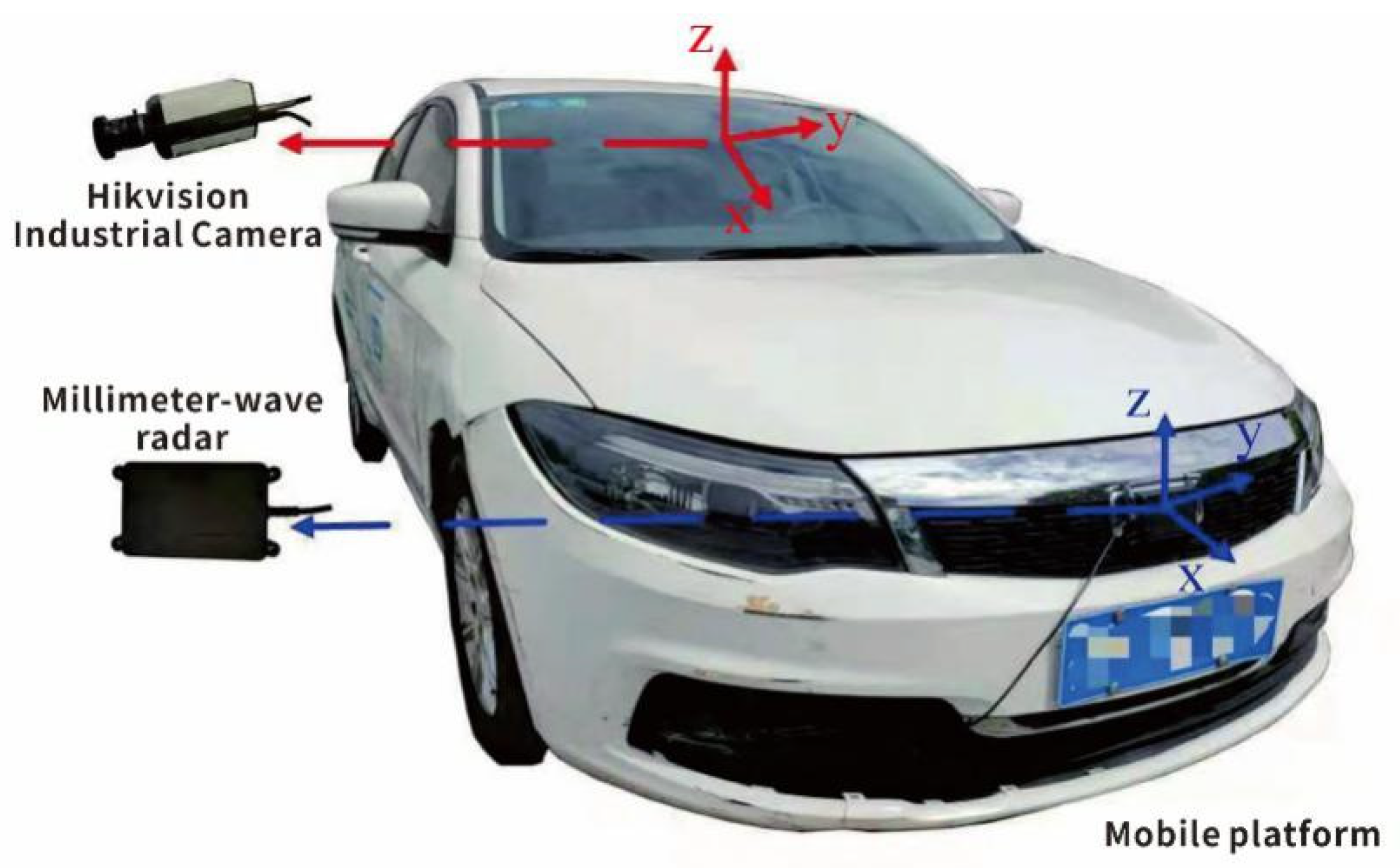
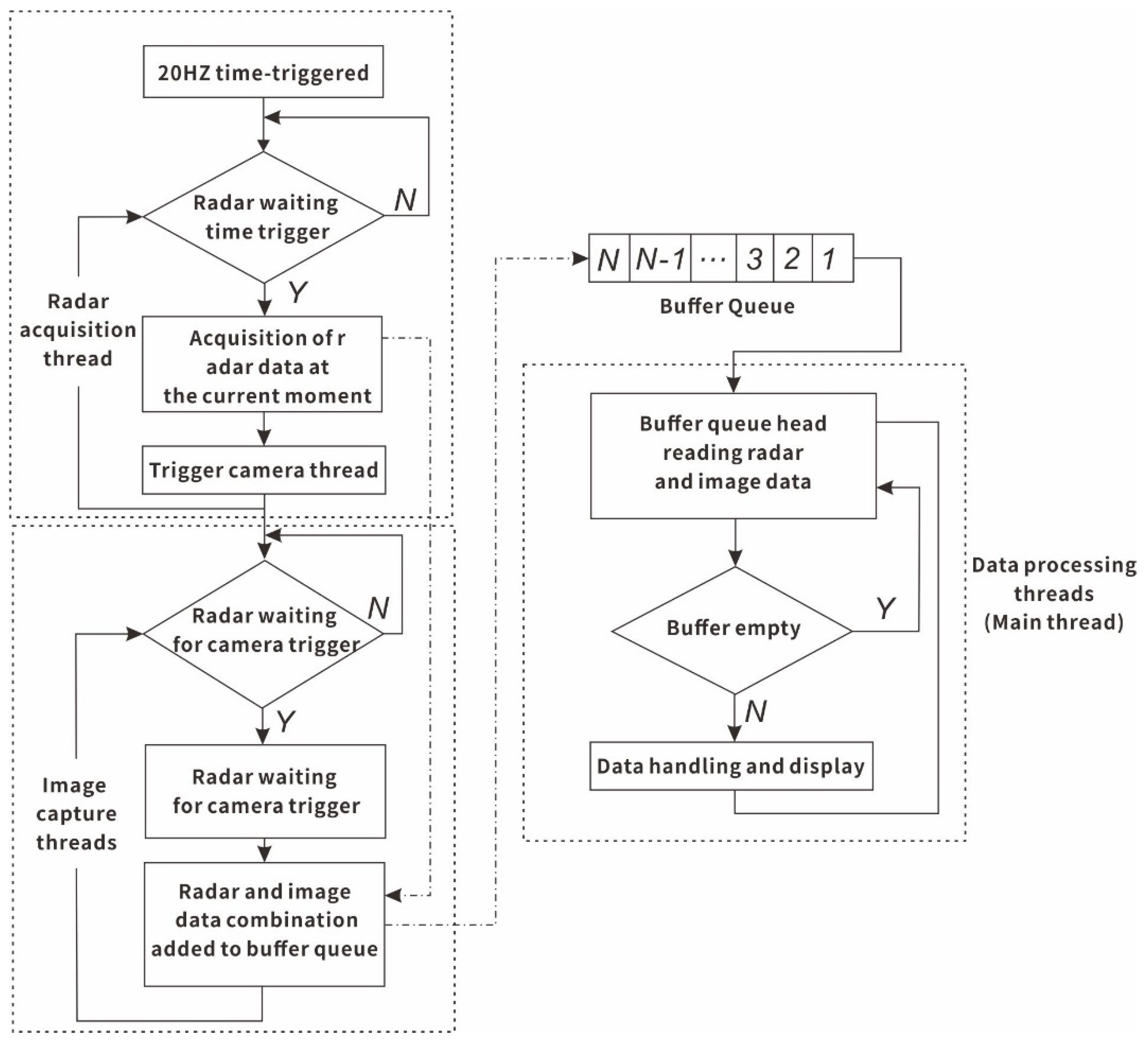
2.1. Algorithm Framework and Data Collection Platform

The algorithm framework in this paper is shown in Figure 1. The millimeter-wave radar was jointly calibrated with the camera to acquire the road environment and collect point cloud and image information. The multimodal data was entered into the vehicle-detection module, fused to perform vehicle detection and output the results.
Then, the vehicle was detected using a combination of Hikvision cameras and 24 GHz millimeter-wave radar. The millimeter-wave radar was fixed in the center of the front bumper of the vehicle and the camera under the rearview mirror, as shown in Figure 2. The NRA24 mm wave radar and the camera have a sampling frequency of 20 Hz and 50 Hz and a data acquisition interval of 50 ms and 50 Hz per frame, respectfully.

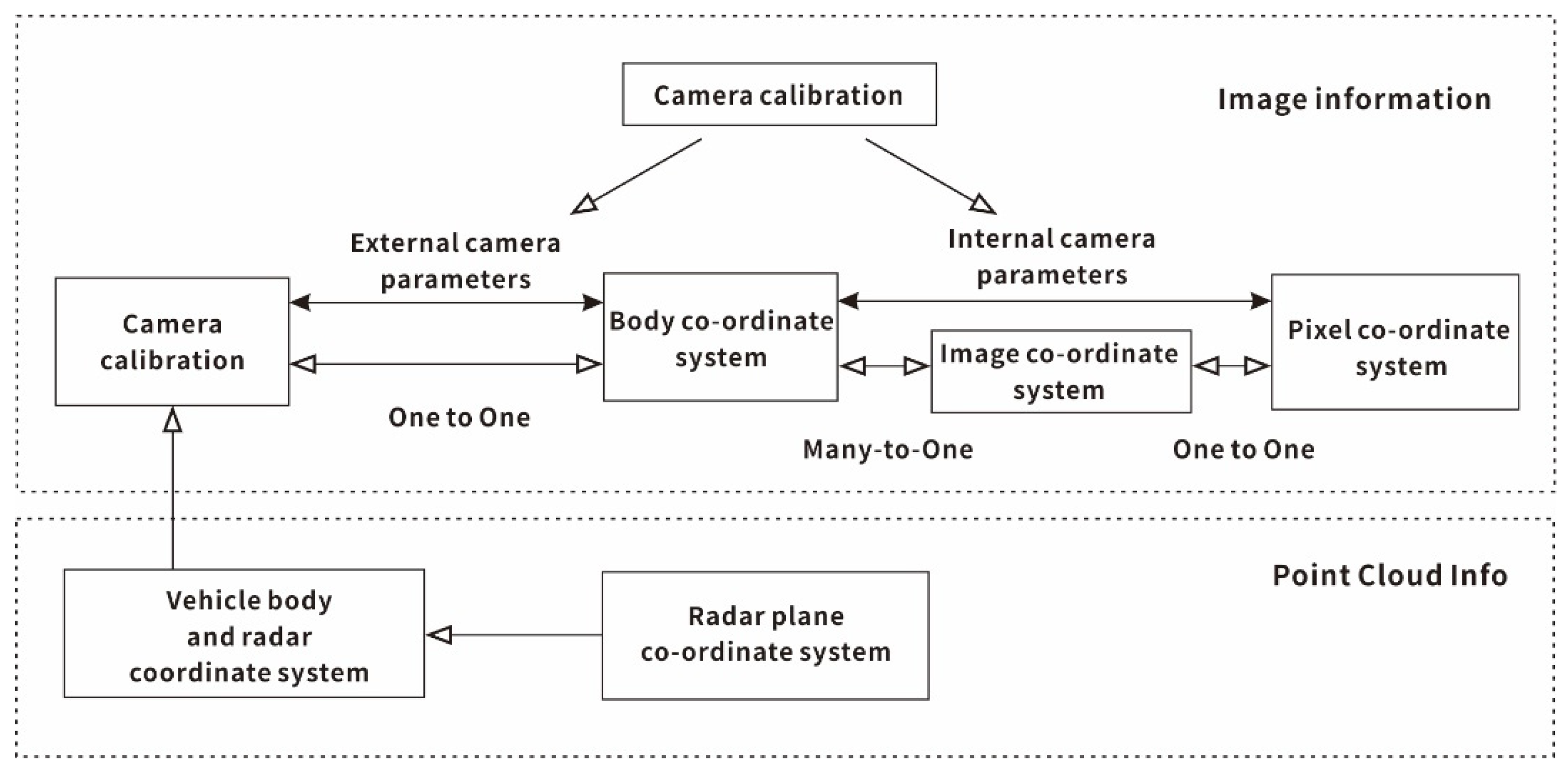
2.2. Millimeter-Wave Radar and Camera Joint Calibration

The joint calibration is a preparatory condition for multimodal fusion. As the millimeter-wave radar and the camera have different sampling frequencies and coordinate systems, the sensor coordinates must be adjusted to the same coordinate system and time has to be aligned before fusion. Furthermore, the spatial calibration of the millimeter-wave radar and the camera requires the concurrent point cloud and the corresponding pixel points in the image.
Based on the assumption that the object point P in the vehicle coordinate system is (x1, y1, z1) and the image point Q in the image coordinate system is (x, y), the pixel-level fusion equation ZC is:
Z C ( x , y , 1 ) T = K ( R c ( x 1 , y 1 , z 1 ) T + Τ c ) .
where the coordinate of object point P is in the Z-axis direction in the camera coordinate system, K is the internal camera parameter matrix and Rc and Tc are the rotation matrix and translation vector of the external camera, respectively.
Millimeter-wave radar presents three-dimensional information as two-dimensional information in a polar coordinate system. If the radial distance between the millimeter-wave radar and the target is R, the angle to the center is α, the plane in which the coordinate system is located is parallel to the environmental coordinate system and the distance between them is H0, then the interconversion relationship of the coordinates of the object point P between the environmental coordinate system (xn, yn, zn) and the millimeter-wave radar coordinate system (R, α) can be expressed as:
{ x n = R sin α y n = H 0 z n = R cos α 0
Combining Equations (1) and (2) yields the transformation between the millimeter-wave radar coordinate system and the image pixel coordinate system as:
z c [ x y 1 ] = [ f x 0 u 0 0 f y υ 0 0   0   1 ] ( R c * [ R sin α H 0 R cos α ] + T c * ) .
The transformation relationship between the spatially calibrated car body coordinate system and the pixel coordinate system is shown in Figure 3.
In this study, time alignment consisted of total data acquisition, millimeter-wave radar data acquisition and image acquisition, where each frame of data was given a system time. The data were transmitted to the buffer queue with a tag. The millimeter-wave radar data acquisition and image acquisition were initiated in the total data acquisition, with low sampling frequency. The image acquisition was triggered for every frame of millimeter-wave radar data acquired, and the image data with the same time tag was selected from the buffer queue to achieve synchronous data acquisition and storage, the process of which is shown in Figure 4.

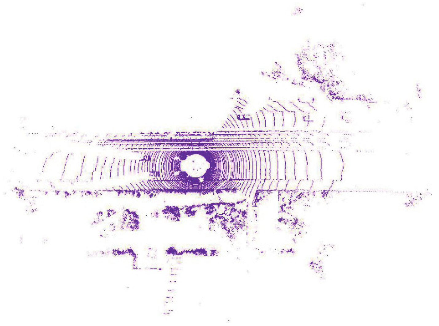
2.3. Statistical Filtering Pre-Processing

When millimeter-wave radar scans a target object, errors in the hardware and software will cause the offset of the 3D coordinates of points within a point set region, then the outliers, and finally redundant feature information and an algorithm model training below the global optimum.
In this study, the curvature tensor was estimated by the least square iterative method and weights were assigned to the samples during the iterations based on the neighborhoods around the point cloud, thus refining each neighborhood around each point. The curvature obtained from the calculation was used along with the statistical weights to recalibrate the normal distribution [24]. The global quantities were minimized, and the curvature and normals were calculated to remove outliers, thus better retaining the texture features of the vehicle point cloud.
In a Cartesian coordinate system, each point of a point cloud exists in x, y and z coordinates. A point cloud sample can be supposed as:
D = { p i R 3 } i = 1 , 2 , , n
where n denotes the total number of sampled point cloud points and pi denotes the unordered points in the sampled sample D. If only the x, y and z coordinates of each unordered point are taken, the distance threshold dmax for the points can be calculated as:
d ¯ i = 1 n i = 1 n d i
σ = 1 n i = 1 n ( d i d ¯ i ) 2 ,
d max = 1 n i = 1 n d i + α × σ .
where di is the distance between two disorder points, d ¯ i is the average distance between the sample disorder points of the point cloud, σ is the sample standard deviation and α is the threshold factor. If the distance between two points is greater than dmax, an outlier occurs and should be excluded from the point set. In our study, the number of proximity points for each point was set to 50, the distance threshold was 1, the threshold coefficient α was 0.5 and the threshold factor α was 0.2.
Figure 5 shows the initial view of the point cloud sample. The point cloud at the near end is scattered, the ground point cloud is not clear, and in the distant point cloud around the obstacle exist more chaotic outliers and uneven distribution, which makes vehicle detection more difficult. Figure 6 shows the view after data preprocessing, where the point distribution in the local area is comparatively more uniform, the ground point cloud at the near end is flat and easy to implement the subsequent ground segmentation, and the distant point only directs to the vehicle and wall point cloud information, uniformly distributed.

3. 3D Vehicle-Detection Algorithm

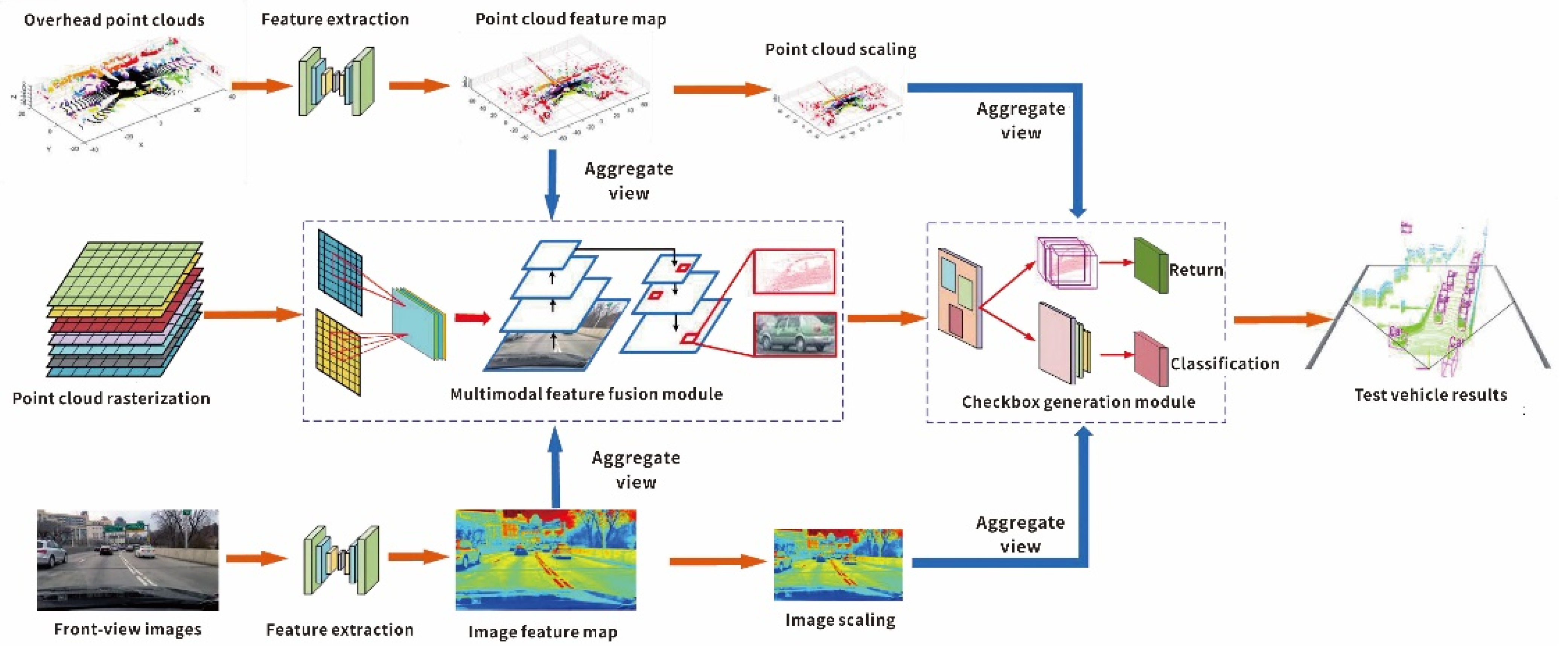
3.1. General Idea of the Algorithm

To address the diversity and complexity of vehicle features, this study introduced a deep neural network to implement vehicle detection. The algorithm framework is shown in Figure 7. At first, the preprocessed point cloud and image information were used for feature extraction using ResNet [25] and multiple views with the same aspect ratio were obtained for feature matching by scaling the size of the point cloud and image feature map. Then, the multimodal feature fusion module was introduced to perform a pixel-by-pixel averaging operation on the multimodal features to achieve multimodal feature fusion, and the feature pyramid [26] was added to extract higher-order features. Finally, the higher-order features were entered into the detection frame generation module and aggregated with the cropped view to generate a 3D vehicle-detection frame.

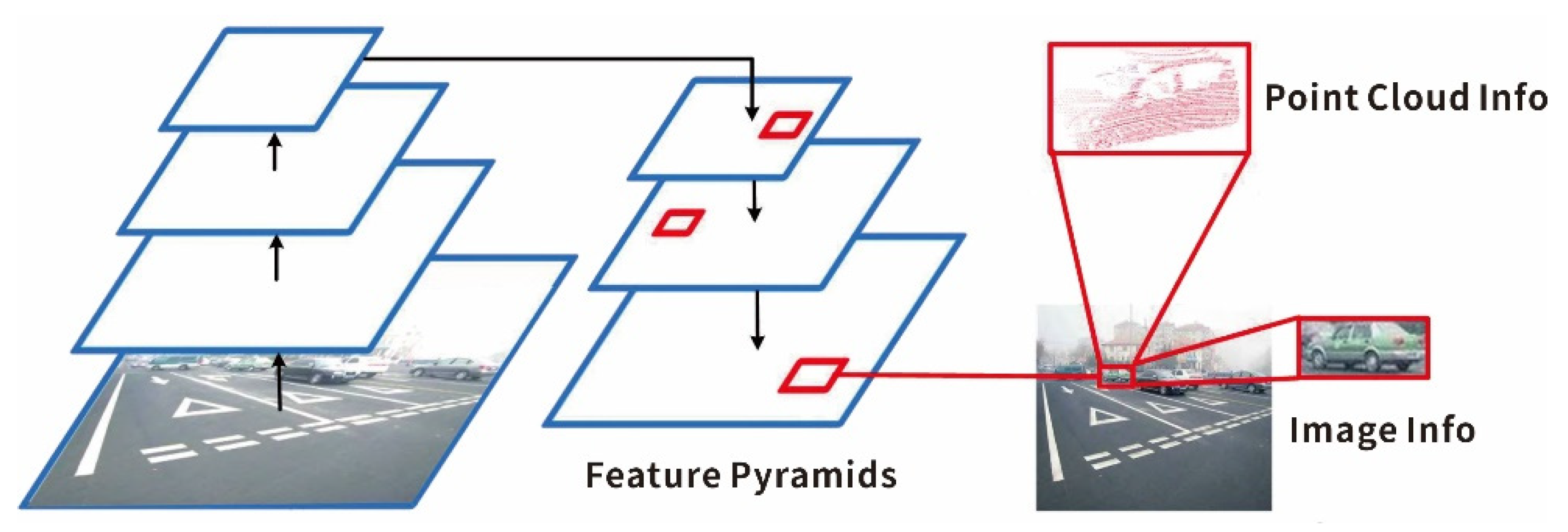
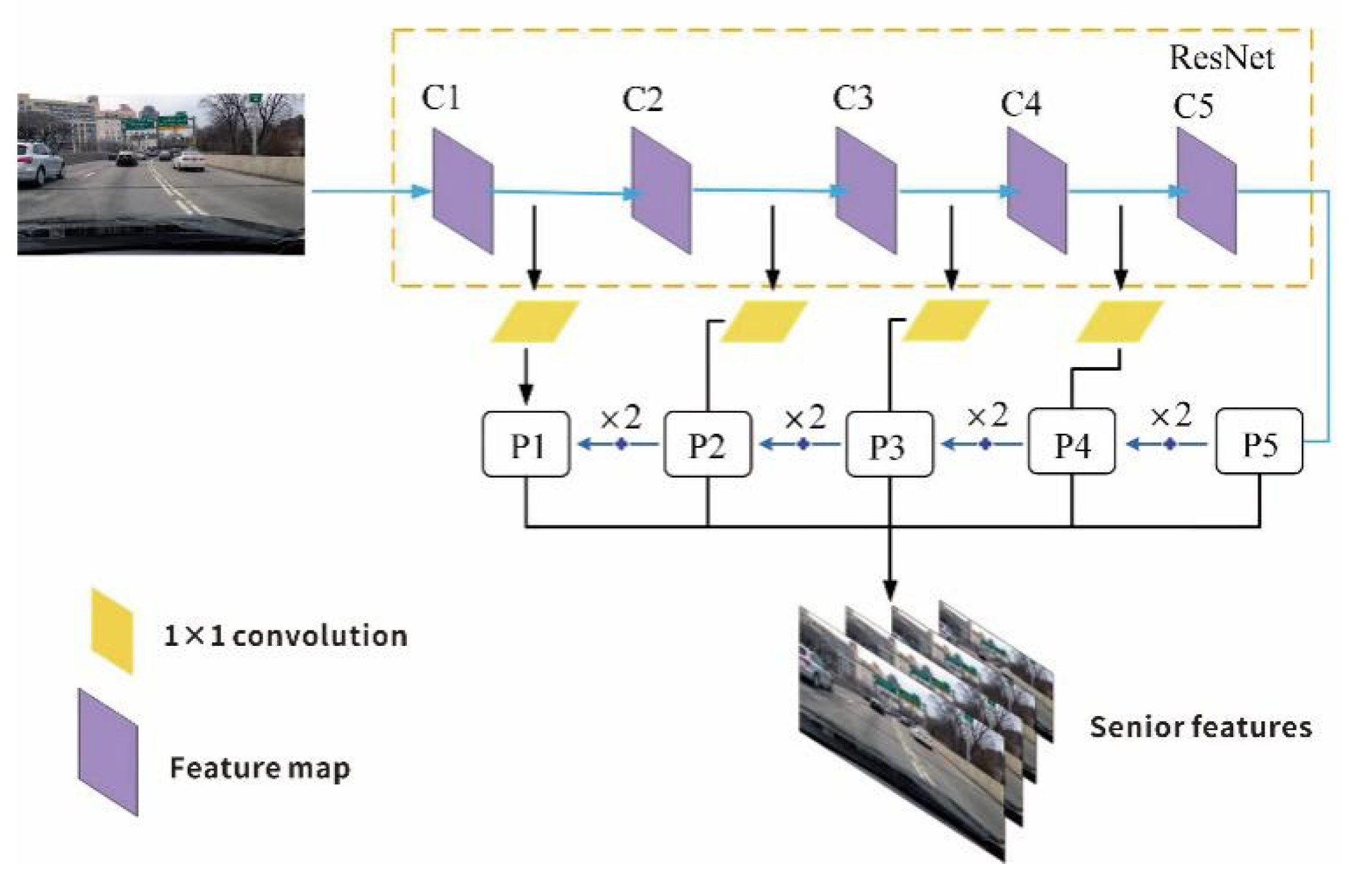
3.2. Multimodal Feature Fusion Module

In this study, the multimodal feature fusion module was constituted by feature fusion, feature pyramids and 1 × 1 convolution. The sparse point cloud after feature extraction was matched with the image and entered into the feature pyramid simultaneously to complete the extraction of target features, which was finally processed by a 1 × 1 convolution to reduce the dimensionality. Moreover, the multimodal feature fusion module was used for region selection and resizing of the input feature values by clipping the uniform resolution. Multiview feature maps were processed with pixel-by-pixel averaging and point cloud information was fused with advanced image information features. The fused image was transmitted into the feature pyramid and upsampled. Moreover, the features were enhanced by connecting them to the previous layer of features and using a horizontal structure, as shown in Figure 8.
Each layer from P1 to P5 produced a feature map, which was used to fuse features with different resolutions and semantic strengths to achieve detection of vehicles with different resolutions, therefore ensuring that each layer had the appropriate resolution and strong semantic features to solve the multiscale problem in vehicle detection. As is shown in Figure 9, the feature pyramid extracted 100,000 7 × 7 features on a 256-dimensional feature map, which greatly increased the computational effort. Besides, the 1 × 1 convolutional reduction was added to the back of the feature pyramid to reduce the number of convolution kernels and that of features without changing the size of the feature map.
Finally, we projected the aggregated fused features onto a six-channel raster with a resolution of 0.1 m. In the process, the first five channels were generated for the same slice within the maximum height of the raster cell, and the sixth channel consisted of the density information for each raster cell.

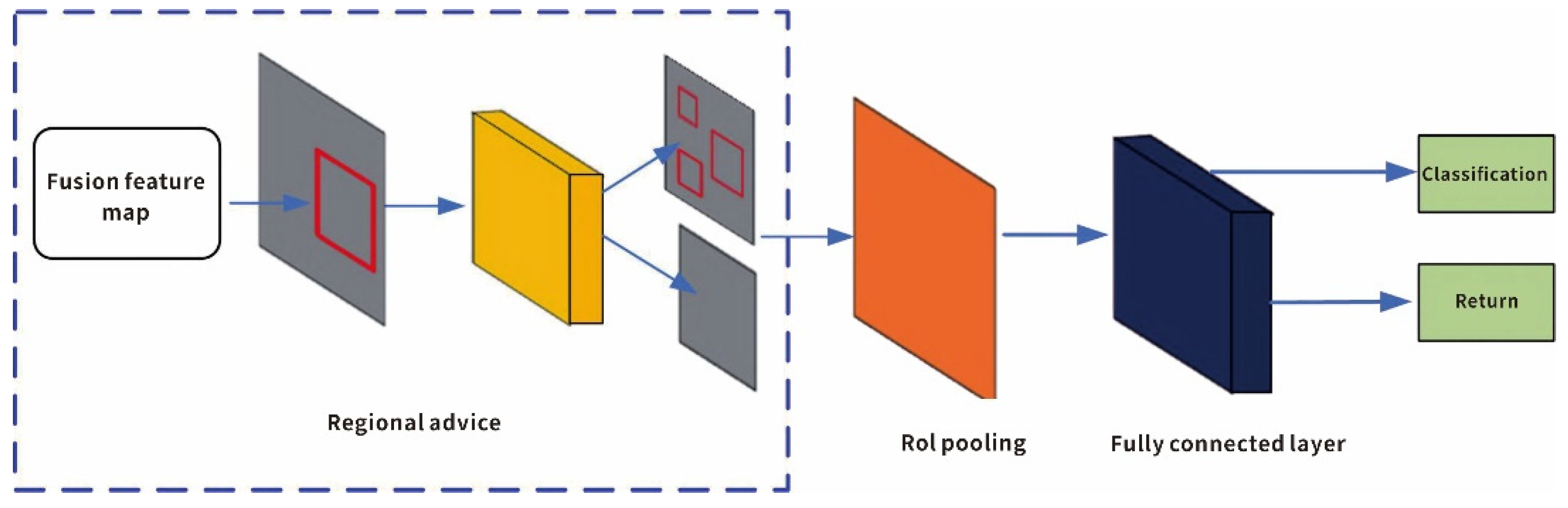
3.3. Checkbox Generation Module

The fused feature information was transmitted to the vehicle detection module to complete the regression and classification. The vehicle detection module was composed of a region suggestion, RoI pooling and a fully connected layer.
This paper adopts a new feature fusion regional structure, as shown in Figure 10. The top view projected onto the raster was used to fuse the incoming region scheme with the main view. RoI pooling scaled the new feature map to 7 × 7 and transmitted it into the fully connected layer to output the regression, direction estimation and category classification of each vehicle-detection frame, direction estimation and class classification. Finally, non-maximum suppression was used to remove redundant 3D detection frames.
This paper introduces a multitasking loss designed for:
L = 1 N c i L c ( 8 i , u i ) + λ 1 1 N p [ u i > 0 ] L r + λ 2 1 N p * L s
where Nc and Np are the number of point cloud points and the number of down-sampled point clouds, respectively, and the classification loss Lc is the cross-entropy loss. Besides, in the following formula:
H ( p , q ) = ( s i log u i + ( 1 s i ) log ( 1 u i ) ) .
where si is the predicted classification score and ui is the label of centroid i.
Since the regression loss Lr includes the distance regression loss Ldist, and the size regression loss Lsize, Ldist and Lsize make the loss function more robust to outliers using the Smooth L1 function, which can be expressed as:
Smooth L 1 = { 0.5 χ 2 , if | x | < 1 | x | 0.5 , otherwise
When angular losses Ls include angular losses Lcorner and angular regression losses Langle, they can be expressed as follows:
L corner = m = 1 8 P m G m
L angle = L c ( d c a , t c a ) + D ( d r a , t r a )
where d c a and d r a are the corresponding residuals and predicted values of the regression, respectively, t r a and t c a are the sample points of the corresponding point cloud, the angular loss is the difference between the eight predicted angles and the labelled values, Pm is the labelled value of point m and Gm is the predicted value of point m.
To eliminate the detection of overlaps, this study adopted a non-maximum suppression with a threshold of 0.7 to remove the large overlapping bounding boxes near the vehicles. The final detection of the box vertex alignment was used for matching to reduce the computational parameters, and the vehicle offset with respect to the ground plane was used to obtain a more accurate 3D rectangular box location.

4. Experimental Results and Analysis

4.1. Platform and Parameters

This experiment was conducted in the TensorFlow framework with an Intel Core i7-6700 computer processor, 32 GiB of RAM and an NVIDIA GeForce RTX 2080Ti for GPU-accelerated training. The learning rate was 0.001 and the training was performed on the KITTI dataset [27] for 120 cycles, each with a decay factor of 1000. Besides, the learning rate was 0.001 and 120 cycles were trained on the KITTI dataset [27], each cycle being 1000 and with a decay factor of 0.8.

4.2. Experimental Results

This study selected the network model with 120 training cycles to verify the multitarget detection capability of the improved network model in different traffic scenarios. The testing results are shown in Figure 11, Figure 12, Figure 13 and Figure 14.
Figure 11 demonstrates the results of vehicle detection in a natural traffic scenario. As is seen, the 3D vehicle-detection algorithm is effective to achieve vehicle detection. The detection results are consistent with the actual determination results and the target calibration frame range is more accurate.
Figure 12 shows the experimental results in the illuminated traffic condition. Specifically, Figure 12a is the result of the shadow occlusion case and Figure 12b is that of the light occlusion case. As is seen, even though the color and texture of the image both greatly change because of the disturbance of strong illumination toward the camera of the vehicle, the method proposed in this paper guarantees successful vehicle detection since the inclusion of multimodal feature fusion makes it possible for the point cloud to provide the needed image information.
Figure 13 shows the experimental results in the complex scenario, specifically of a distant vehicle in Figure 13a and an obscured vehicle in Figure 13b. This indicates that the method proposed in this paper shows its effectiveness in detecting multiple targets and great stability in dealing with the complex situation of multiple targets.
Figure 14 provides the results in the complex roadway scenario—Figure 14a in a one-way roadway and Figure 14b in an intersecting roadway. The vehicle point cloud features are not distinctive because of the complex road conditions, such as vehicle occlusions and the oncoming, outgoing and lateral vehicles in different directions. According to the experimental results, the vehicle-detection accuracy in the complex conditions can be ensured through the acquisition of 2D information from the camera and the matching of the vehicle’s position in the 3D environment by the millimeter-wave radar.
Based on all the above results, the algorithm adopted in this paper is effective in detecting either obscured, illuminated or multiscale, multitarget vehicles by making up for the lack of cameras and millimeter-wave radar through multimodal fusion, no matter if it is in natural or complex road conditions.
Figure 15 shows the network training loss and detection accuracy, where models in iteration periods of 60, 80, 100 and 120 were evaluated. As the training period lengthens and the learning rate changes, the network loss will effectively decrease and converge, indicating that the detection accuracy of the improved network model increases (see Table 1).
In this study, the algorithm was compared with the current mainstream algorithm in the same dataset and condition, the results of which are shown in Table 2. In the comparison experiments, the 3D detection methods were divided into the original point cloud method, multiview method and image point cloud fusion method. The main algorithms in the different methods were differentiated but tested on the same KITTI dataset. The average detection accuracy of the algorithms was 84.71%. However, the small amount of redundant data and the low dimensionality of the classification features produce a higher accuracy in the method adopting this algorithm than in the others. Due to the inclusion of the feature pyramid, the detection time is slightly longer in the method than in the others adopting the original point cloud-based Complexer-YOLO and 3DSSD algorithms, which is still a result better than those in the other mainstreams.
The results produced by one algorithm individually in the original point cloud method, multiview method and image point cloud fusion method were selected to compare those produced in the method adopting our proposed algorithm, which is shown in Figure 16. In the cases with shadow occlusion, vehicle occlusion and distant vehicles, the false detection rate and missed detection rate are both lower and the 3D detection frame-matching accuracy of the vehicles is higher in the method adopting this algorithm than in the other three methods. The experimental results indicate that the proposed algorithm provides fast and accurate 3D vehicle detection in both natural and complex scenarios, meaning it is an effective and feasible method.

5. Conclusions

In this paper, a multimodal feature fusion approach was employed to detect vehicles by fusing multimodal features from cameras and millimeter-wave radar. The algorithm introduced a statistical filtering algorithm to preprocess and remove redundant information from the point cloud. It improved the vehicle-detection accuracy in complex road scenarios after the process of fusing multimodal features, combining them with a feature pyramid to extract higher-level features, and finally using area suggestions to match the 3D detection frame to generate a vehicle-detection frame. The vehicle recognition accuracy of the algorithm was 84.71%, showing a good stability in natural and complex road scenarios. The average total processing time for a single frame of fused data was 0.14 s, showing a good real-time performance. The algorithm enables the unmanned system to achieve 3D vehicle-detection in complex road scenarios.

Author Contributions

Visualization, N.C.; Writing—original draft, Y.W.; Writing—review & editing, H.L. All authors have read and agreed to the published version of the manuscript.

Funding

This research received no external funding.

Institutional Review Board Statement

Not applicable.

Informed Consent Statement

Not applicable.

Conflicts of Interest

The authors declare no conflict of interest.

References

  1. Cai, P.D.; Wang, S.K. Probabilistic end-to-end vehicle navigation in complex dynamic environments with multimodal sensor fusion. IEEE Robot. Autom. Lett. 2020, 5, 4218–4224. [Google Scholar] [CrossRef]
  2. Liu, Y.X.; Wu, X.; Xue, G. Real-time detection of road traffic signs based on deep learning. J. Guangxi Norm. Univ. (Nat. Sci. Ed.) 2020, 38, 96–106. [Google Scholar]
  3. Zhang, Y.; Song, B. Vehicle tracking using surveillance with multimodal data fusion. IEEE Trans. Intell. Transp. Syst. 2018, 19, 2353–2361. [Google Scholar] [CrossRef] [Green Version]
  4. Stanislas, L.; Dunbabin, M. Multimodal sensor fusion for robust obstacle detection and classification in the maritime RobotX challenge. IEEE J. Ocean. Eng. 2019, 44, 343–351. [Google Scholar] [CrossRef] [Green Version]
  5. Xie, D.S.; Xu, Y.C. 3D LIDAR-based obstacle detection and tracking for unmanned vehicles. Automot. Eng. 2020, 56, 165–173. [Google Scholar]
  6. Xue, P.L.; Wu, W. Real-time target recognition of urban autonomous vehicles based on information fusion. J. Mech. Eng. 2020, 56, 165–173. [Google Scholar]
  7. Zheng, S.W.; Li, W.H. Vehicle detection in traffic environment based on laser point cloud and image information fusion. J. Instrum. 2019, 40, 143–151. [Google Scholar]
  8. Wang, G.J.; Wu, J. 3D vehicle detection with RSU LiDAR for autonomous mine. IEEE Trans. Veh. Technol. 2021, 70, 344–355. [Google Scholar] [CrossRef]
  9. Dai, D.Y.; Wang, J.K. Image guidance based 3D vehicle detection in traffic scene. Neurocomputing 2021, 428, 1–11. [Google Scholar] [CrossRef]
  10. Chen, L.; Si, Y.W. 3D LiDAR-based driving boundary detection of unmanned vehicles in mines. J. Coal 2020, 45, 2140–2146. [Google Scholar]
  11. Choe, J.S.; Joo, K.D. Volumetric propagation network: Stereo-LiDAR fusion for long-range depth estimation. IEEE Robot. Autom. Lett. 2021, 6, 4672–4679. [Google Scholar] [CrossRef]
  12. Zhang, C.L.; Li, Y.R. A chunking tracking algorithm based on kernel correlation filtering and feature fusion. J. Guangxi Norm. Univ. (Nat. Sci. Ed.) 2020, 38, 12–23. [Google Scholar]
  13. Nie, J.; Yan, J. A multimodality fusion deep neural network and safety test strategy for inelligent vehicles. IEEE Trans. Intell. Veh. 2021, 6, 310–322. [Google Scholar] [CrossRef]
  14. Zhang, X.Y.; Li, Z.W. Channel attention in LiDAR-camera fusion for lane line segmentation. Pattern Recognit. 2021, 118, 108020. [Google Scholar] [CrossRef]
  15. Wang, X.; Li, K.Q. Intelligent vehicle target parameter identification based on 3D LiDAR. Automot. Eng. 2016, 38, 1146–1152. [Google Scholar]
  16. Li, M.L.; Wang, L. Point cloud plane extraction using octonionic voxel growth. Opt. Precis. Eng. 2018, 26, 172–183. [Google Scholar]
  17. Wu, Y.H.; Liang, H.W. Adaptive threshold lane line detection based on LIDAR echo signal. Robotics 2015, 37, 451–458. [Google Scholar]
  18. Chen, Z.Q.; Zhang, Y.Q. An improved DeepSort target tracking algorithm based on YOLOv4. J. Guilin Univ. Electron. Sci. Technol. 2021, 41, 140–145. [Google Scholar]
  19. Ding, M.; Jiang, X.Y. A monocular vision-based method for scene depth estimation in advanced driver assistance systems. J. Opt. 2020, 40, 1715001. [Google Scholar]
  20. Peng, B.; Cai, X.Y. Vehicle recognition based on morphological detection and deep learning for overhead video. Transp. Syst. Eng. Inf. 2019, 19, 45–51. [Google Scholar]
  21. Cheng, H.B.; Xiong, H.M. YOLOv3 vehicle recognition method based on CIoU. J. Guilin Univ. Electron. Sci. Technol. 2020, 40, 429–433. [Google Scholar]
  22. Zhao, X.M.; Sun, P.P. Fusion of 3D LIDAR and camera data for object detection in autonomous vehicle applications. IEEE Sens. J. 2020, 20, 4901–4913. [Google Scholar] [CrossRef] [Green Version]
  23. Zhe, T.; Huang, L.Q. Inter-vehicle distance estimation method based on monocular vision using 3D detection. IEEE Trans. Veh. Technol. 2020, 69, 4907–4919. [Google Scholar] [CrossRef]
  24. Pourmohamad, T.; Lee, H.K.H. The statistical filter approach to constrained optimization. Technometrics 2020, 62, 303–312. [Google Scholar] [CrossRef]
  25. He, K.M.; Zhang, X.Y. Deep residual learming for image recognition. In Proceedings of the 2016 IEEE Conference on Computer Vision and Patten Recognition (CVPR), Las Vegas, NV, USA, 26 June–1 July 2016. [Google Scholar]
  26. Lin, T.Y.; Dollár, P.; Girshick, R.; He, K.; Hariharan, B.; Belongie, S. Feature pyramid networks for object detection. In Proceedings of the 2017 IEEE Conference on Computer Vision and Pattern Recognition (CVPR), Honolulu, Hawaii, 21–26 July 2017. [Google Scholar]
  27. Geiger, A.; Lenz, P. Vision meets robotics: The KITTI dataset. Int. J. Robot. Res. 2013, 32, 1231–1237. [Google Scholar] [CrossRef] [Green Version]
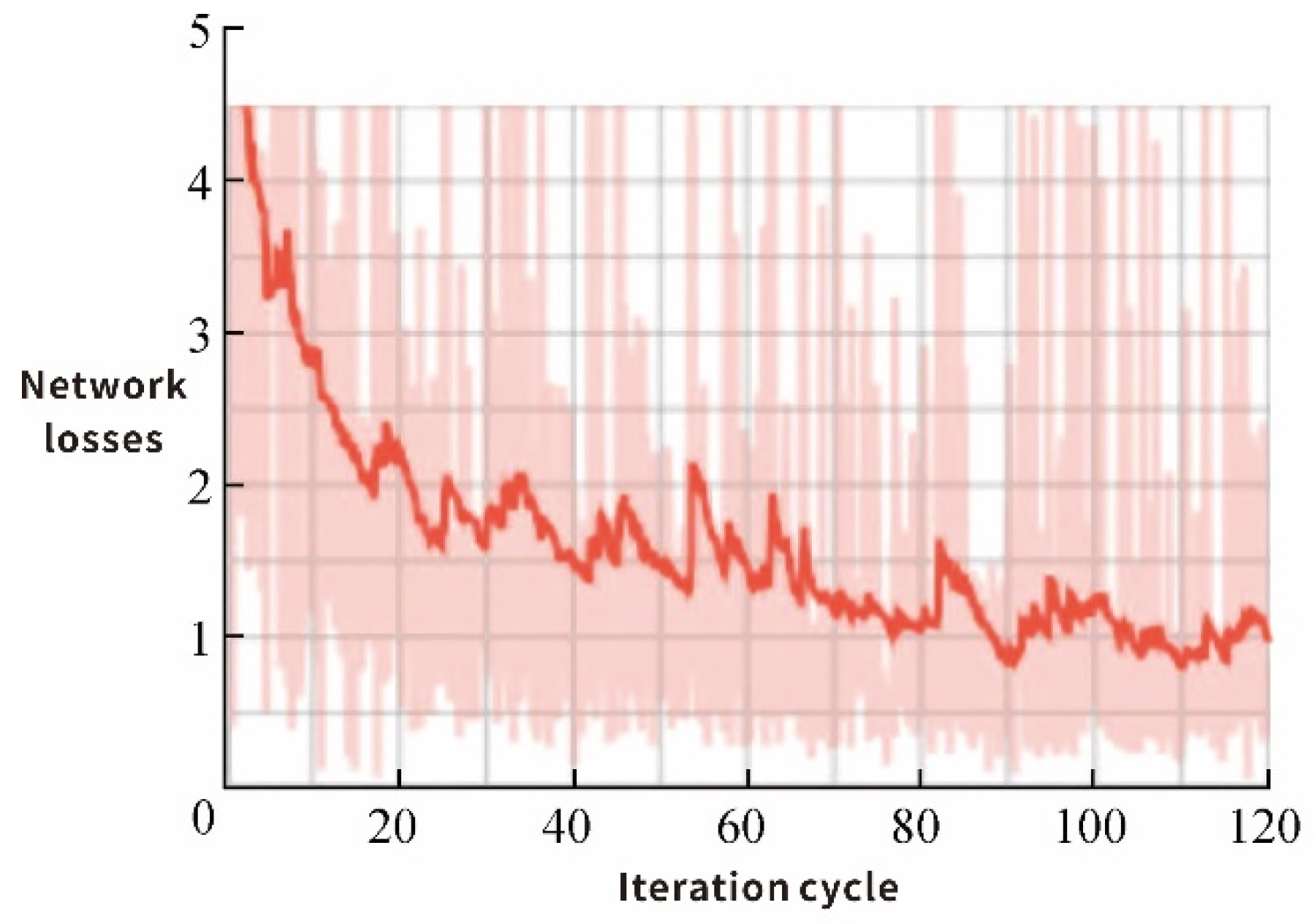
Figure 1. Framework of vehicle-detection algorithm.
Applsci 12 06198 g001
Figure 2. Diagram of sensor installation.
Applsci 12 06198 g002
Figure 3. Diagram of coordinate system conversion.
Applsci 12 06198 g003
Figure 4. Flowchart of time registration.
Applsci 12 06198 g004
Figure 5. Point cloud data before filtering.
Applsci 12 06198 g005
Figure 6. Point cloud data after filtering.
Applsci 12 06198 g006
Figure 7. Algorithm framework.
Applsci 12 06198 g007
Figure 8. Feature pyramid network.
Applsci 12 06198 g008
Figure 9. Advanced feature extraction.
Applsci 12 06198 g009
Figure 10. Feature fusion area suggestion module.
Applsci 12 06198 g010
Figure 11. Natural scene experiment results: (a) one-way oncoming traffic; (b) two-way oncoming traffic; (c) wide road; and (d) narrow roads.
Applsci 12 06198 g011
Figure 12. Illumination scene experiment results: (a) shade shading; and (b) light blocking.
Applsci 12 06198 g012
Figure 13. Multitarget scene experiment results: (a) long-range vehicles; and (b) blocking of vehicles.
Applsci 12 06198 g013
Figure 14. Complex road section scene detection results: (a) one-way section; and (b) crossroads.
Applsci 12 06198 g014
Figure 15. Training loss chart.
Applsci 12 06198 g015
Figure 16. Algorithm effect comparison diagram.
Applsci 12 06198 g016
Table 1. Network training loss and detection accuracy.
Training CyclesNetwork LossesTesting Accuracy%
601.65273.32
801..27179.46
1001.39383.84
1201.13284.71
Table 2. Comparison of time and accuracy of mainstream algorithms.
Testing MethodsAlgorithmsPrecision%Time/sAverage Accuracy%
SimpleGeneralDifficulties
Raw point cloud methodComplexer-YOLO24.2718.5317.310.0920.04
3DSSD88.3679.5774.550.1080.83
VOXEL3D86.4577.6972.200.2478.78
Multi-view approachSARPNET85.6376.6471.310.1277.86
SIE Net88.2281.7177.220.1582.38
MVOD88.5380.0177.240.1681.93
Image point cloud fusion methodsF-PointNet82.1969.7960.590.1770.86
AVOD83.0771.7665.730.2273.52
MV3D74.9763.6354.000.3664.20
Text Algorithms88.7585.5279.860.1484.71
Publisher’s Note: MDPI stays neutral with regard to jurisdictional claims in published maps and institutional affiliations.

