Article

Optimal Placement of Vibration Sensors for Industrial Robots Based on Bayesian Theory

1
School of Mechanical Engineering, Xi’an Jiaotong University, Xi’an 710049, China
2
Shaanxi Key Laboratory of Intelligent Robots, Xi’an Jiaotong University, Xi’an 710049, China
*
Author to whom correspondence should be addressed.
Appl. Sci. 2022, 12(12), 6086; https://doi.org/10.3390/app12126086
Submission received: 7 May 2022 / Revised: 12 June 2022 / Accepted: 13 June 2022 / Published: 15 June 2022
(This article belongs to the Special Issue Advanced Manufacturing Technologies and Their Applications, Volume II)

Abstract

:
This paper presents an optimal sensor placement method for vibration signal acquisition in the field of industrial robot health monitoring and fault diagnosis. Based on the general formula of Bayes and relative entropy, the evaluation function of sensor placement is deduced, and the modal confidence matrix is used to express the redundancy of sensor placement. The optimal placement of vibration sensors is described as a discrete variable optimization problem, which is defined as whether the existing sensor layout can obtain joint state information efficiently. The initial layout of the sensor was obtained from the structural simulation results of the industrial robots, and the initial layout was optimized by the derived objective function. The efficiency of the optimized layout in capturing joint state information is proven by the validation experiment with a simulation model. The problem of popularizing the optimization method in engineering is solved by a verification experiment without a simulation model. The optimal sensor placement method provides a theoretical basis for industrial robots to acquire vibration data effectively.

1. Introduction

1.1. Background and Significance of the Study

As more and more robots are introduced into space, industry, and private homes, fault monitoring is becoming a more critical problem. In the past 30 years, fault monitoring and diagnosis methods for various nonlinear systems and robotic systems have been studied. Model-based analytical redundancy methods have been used for fault detection and isolation of nonlinear and robot systems [1,2,3].
The purpose of fault detection technology is to generate fault-sensitive diagnostic signals. In existing automatically controlled systems, faults can occur in both the mechanical and electrical parts of the plant. Fault isolation allows fault-related inputs to be located from all other system inputs and generates specific residual signals for each fault. For example, in an electromechanical system, such as a robot, a single fault may occur in a specific driver, a specific sensor, or a system on a specific component [4,5].
For multi-joint robots, dynamics [6], kinematics [7], joint clearance [8], and friction models [9] have been studied. The results show that the mechanical transmission system is an essential part of multi-joint robots to transmit motion and force [10].
When the transmission accuracy of the robot is reduced, the working efficiency and output product quality decrease, and the positioning accuracy of the robot is also affected by various factors. Therefore, when the sensors are arranged, the motion state information of the joints should be captured as efficiently as possible. In theory, how to define the validity of sensor distribution is the core of solving this problem.

1.2. Related Work

Juri [11] proposed a greedy frame sense algorithm to select the optimal sensor location when estimating parameters from the measured data of sensors. This algorithm is the first one that is close to optimal in the mean square error.
In the last 10 years, the optimal placement of sensors in mechanical systems and structures has become a hot research topic. Applications include modeling, identification, fault detection, and active control of systems, such as bridges [12]. To ensure safety and functionality, more and more structures are equipped with various types of sensors, such as accelerometers, displacement sensors, strain gauges, and fiber optic sensors for monitoring [13]. The modal confidence matrix is an excellent tool for evaluating the correlation of modal shape vector space. The calculated scalar value is between 0~1 or expressed as a percentage. For industrial robots, the redundancy of sensor placement can be evaluated using a modal confidence matrix.
Yi [14] proposed a hybrid optimization method to optimize sensor placement when constructing an effective structural health detection system. In this method, the modal confidence matrix is introduced, and dual structure coding based on a generalized genetic algorithm is used to determine the sensor position. Hanis [15] argued that sensor configurations should also minimize unnecessary high-mode spillovers in addition to the classic EFI approach. Castro-Triguero [16] used four classical sensor location methods: two based on the Fisher information matrix and two based on the rank optimization of the energy matrix. Methods based on information theory have been developed to provide reasonable solutions to the problem of selecting the optimal sensor configuration in modal identification and structural parameter estimation [17,18]. Li [19] considered that, in the sensor placement of the structural health monitoring system, the structural array and natural frequency should be considered, along with the degree of participation in the structural response. Therefore, a sensor placement method considering both the dynamic characteristics of the structure and the actual load conditions is proposed, and it is verified that the method has a better modal identification effect. Brehm [20] focused on the problem of determining the optimal reference sensor position under random excitation in a weakly stationary process, combined with the set design variables of the sensor location, and the genetic algorithm was used to avoid evaluating all possible combinations of reference sensor positions. The proposed method was verified by a numerical benchmark study of a supported beam and a practical sample. David used a theoretical estimation framework to calculate the optimal geometric sensor formations that would yield the best achievable performance in terms of target positioning accuracy by maximizing the determinant of the appropriately defined Fisher Information Matrix (FIM) [21].
Flynn [22] considered the optimal sensor placement problem in structural health inspections. Based on the general Bayes formula, optimal placement was established as a process of minimizing the expectation of specific errors. Finally, the optimal solution generated by the algorithm was discussed. Using the influence of spatial correlation prediction error on optimal placement, Costas Papadimitriou [23] used information entropy as the performance measure of sensor configuration, and he expressed the optimal position of sensors as the optimization problem of discrete variables, which solved the problem of modal identification and parameter estimation of the structure-related model. Sun Hao [24] transformed the optimization problem into an integer optimization problem and then proposed a discrete optimization scheme based on an artificial bee colony algorithm to solve the optimization problem.
Health monitoring and fault diagnosis of industrial robots are essential for safe and reliable operation, and a practical sensor layout is essential for fault diagnosis and other work. From the above situation, it can be concluded that most of the existing sensor placement methods are based on an optimization algorithm or optimization matrix, and the objective function cannot meet the functional characteristics of industrial robots. Furthermore, as flexible equipment, the operational characteristics and the error problem in the process of sensor signal acquisition need to be considered.
To solve the sensor placement problem of industrial robots, we propose the importance of joint state information acquisition in this paper, and the optimal sensor placement method for joint state information acquisition and its corresponding theoretical framework is proposed. By simultaneously interpreting the error between the velocity and the actual velocity of the distribution theory and the posterior probability of the joint motion, the evaluation function of the sensor placement based on relative entropy is derived. The constraint function is established by using the modal confidence matrix of different sensor layouts. Finally, the evaluation function is combined with the constraint function as the objective function of the sensor placement. This is the first time in the field of industrial robot fault diagnosis and health assessment. The motion state of joints can be obtained more effectively by this method, which is of great significance to the fault diagnosis and health assessment of industrial robots.

2. Sensor Placement Method

First, the kinematic and dynamic simulation of the industrial robot is considered in this study. Through the simulation, the deformation nephogram of the industrial robot and the velocity distribution at different positions can be obtained. The position of the sensor placement is determined by the Bayesian optimal design, which is realized by maximizing the information gain of joint motion state information.

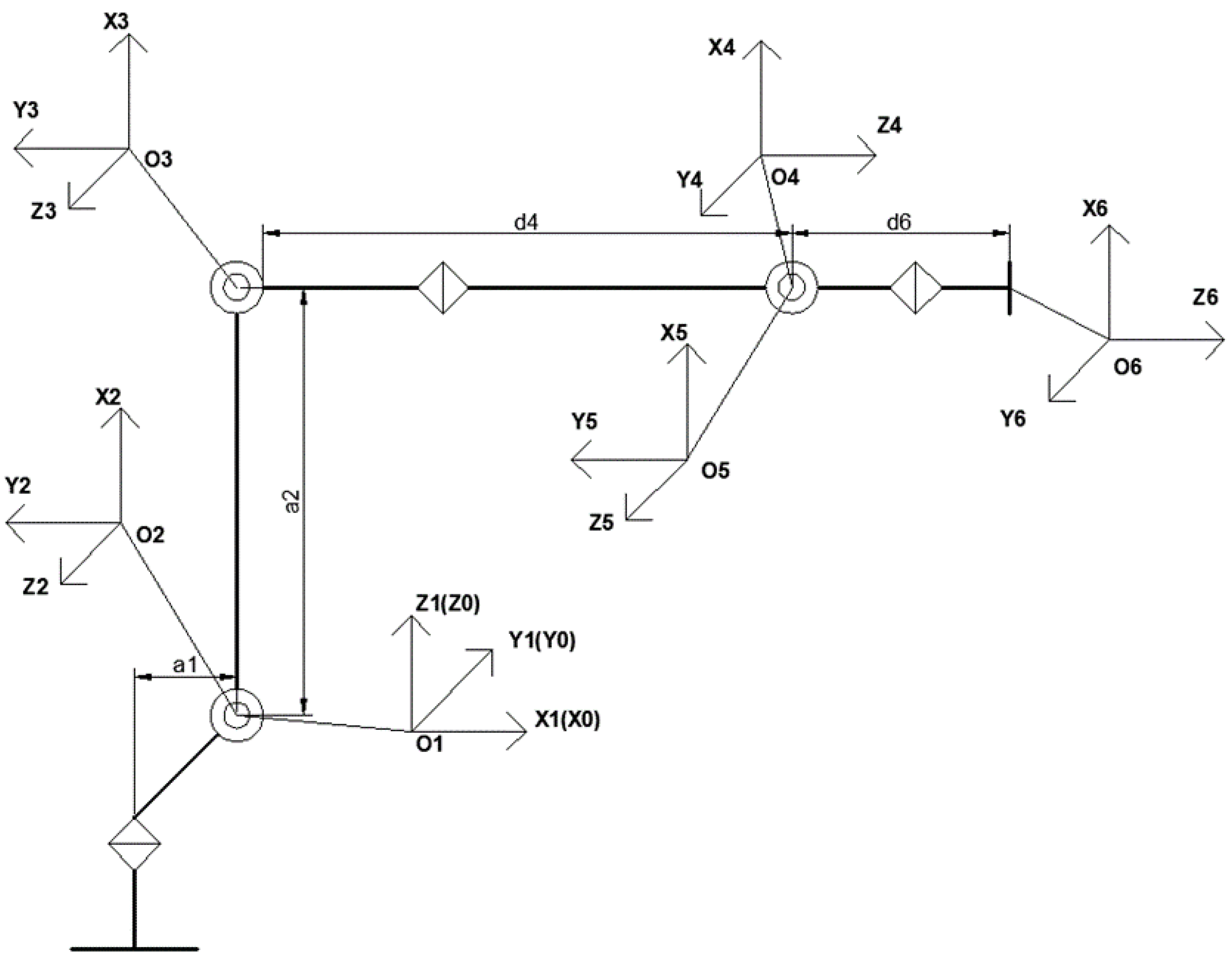
2.1. Derivation of Forward Kinematics of Industrial Robots

The mechanical arm of the six-axis industrial robot used in the simulation in this paper is assembled by a series of connecting rods, so a corresponding coordinate system should be constructed to express the robot. At present, the two commonly used link coordinate system construction methods in robotics are the standard type and the improved D-H coordinate system. Among them, the improved D-H refers to adding a new parameter on the basis of the standard four parameters, through which the singularity that occurs when the adjacent connecting rods are in a parallel relationship can be solved. Since the general six-axis industrial robot does not have parallel links, an improved D-H coordinate system that uses more parameters is not used.
On the other hand, in the existing standard D-H coordinate system, there are also two different establishment methods. The first is that the origin of the coordinate system o i - 1 is unified with the joint i ; the corresponding second is that the coordinate system o i 1 is unified with the joint i 1 . Due to the problem of the tree structure, the first coordinate system will be ambiguous when dealing with it. Considering the diversity of industrial robots, the second method of establishing a system was chosen after a comprehensive comparison. The first method of establishing a system is described in detail below, and the MATLAB model effects corresponding to the two coordinate systems are given.
The establishment method of the connecting rod coordinate system o i x i y i z i is shown in Table 1.
The coordinate system fixed on the robot base (link 0) is coordinate system {0}. This coordinate system has the property of being invariant and can be used as a reference. The reference coordinate system {0} itself is not specially set, but considering the subsequent calculation, the reference coordinate system {0} is set to coincide with the coordinate system {1}. For the revolute joint n, θ n is set to 0.
According to the coordinate system establishment criteria described in this paper, the connecting rod coordinate system of the six-axis industrial robot is solved, as shown in Figure 1.
The link coordinate system of the industrial robot contains 4 parameters. They are defined as follows:
1.
Link length a i : along the x i axis, the distance from z i 1 to z i ;
2.
The torsion angle α i of the connecting rod: the angle from z i 1 to z i around the x i axis;
3.
Link offset d i : along the z i axis, the distance from x i - 1 to x i ;
4.
Joint angle θ i : the angle of rotation from x i - 1 to x i around the z i axis.
For a rotary joint, due to its joint characteristics, it is considered that the definitions of its link length a i , link torsion angle α i and link offset d i are unified, and the joint angle θ i is a joint variable.
Considering the established six-axis industrial robot model, the model parameters need to be calculated according to the specified connecting rod parameter calculation method.
For the six-axis industrial robot model shown in Figure 1, the corresponding link D-H parameters are calculated, as shown in Table 2. Through the D-H parameters of the industrial robot in the table, the configuration of the connecting rod of the industrial robot can be described, which can provide calculation support for the subsequent kinematics analysis and provide importable related parameters for the subsequent kinematics and dynamics simulation.
T i i 1 is defined as: According to the description method of homogeneous transformation of robotic transformation matrix, T i i 1 can be obtained according to the principle from left to right:
T i i 1 = [ c θ i s θ i 0 a i 1 s θ i c α i 1 c θ i c α i 1 s α i 1 s α i 1 d i s θ i s α i 1 c θ i s α i 1 c α i 1 c α i 1 d i 0 0 0 1 ]
The parameters corresponding to each joint are brought in, and the motion transfer matrix of each joint is solved as follows:
T 1 0 = [ c 1 s 1 0 0 s 1 c 1 0 0 0 0 1 0 0 0 0 1 ] T 2 1 = [ c 2 s 2 0 0 0 0 1 0 s 2 c 2 0 0 0 0 0 1 ] T 3 2 = [ c 3 s 3 0 a 2 s 3 c 3 0 0 0 0 1 0 0 0 0 1 ] T 4 3 = [ c 4 s 4 0 0 0 0 1 d 4 s 4 c 4 0 0 0 0 0 1 ] T 5 4 = [ c 5 s 5 0 0 0 0 1 0 s 5 c 5 0 0 0 0 0 1 ] T 6 5 = [ c 6 s 6 0 0 0 0 1 d 6 s 6 c 6 0 0 0 0 0 1 ]
where s i = sin θ i , c i = cos θ i .
After obtaining the transformation matrix of the connecting rod coordinate system, the kinematic equation of the industrial robot is derived. The overall transfer matrix is T 0 6 , and the expression of is:
0 T 6 = T 0 1 T 1 2 T 2 3 T 3 4 T 4 5 T 5 6 = [ n x o x a x p x n y o y a y p y n z o z a z p z 0 0 0 1 ]
n x = s 6 ( c 4 s 1 + s 4 ( c 1 c 2 c 3 c 1 s 2 s 3 ) ) c 6 ( c 5 ( s 1 s 4 c 4 ( c 1 c 2 c 3 c 1 s 2 s 3 ) ) + s 5 ( c 1 c 2 s 3 + c 1 s 2 c 3 ) n y = s 6 ( c 4 c 1 + s 4 ( s 1 s 2 s 3 c 2 c 3 s 1 ) ) + c 6 ( c 5 ( c 1 s 4 c 4 ( s 1 s 2 s 3 c 2 c 3 s 1 ) ) s 5 ( c 2 s 3 s 1 + c 3 s 1 s 2 ) n z = s 4 s 6 ( c 2 s 3 + c 3 s 2 ) c 6 ( s 5 ( c 2 c 3 s 2 s 3 ) + c 4 c 5 ( c 2 s 3 + c 3 s 2 ) ) o x = s 6 ( c 5 ( s 1 s 4 c 4 ( c 1 c 2 c 3 c 1 s 2 s 3 ) ) + s 5 ( c 1 c 2 s 3 + c 1 c 3 s 2 ) ) c 6 ( c 4 s 1 + s 4 ( c 1 c 2 c 3 c 1 s 2 s 3 ) ) o y = c 6 ( c 1 c 4 + s 4 ( s 1 s 2 s 3 c 2 c 3 s 1 ) ) s 6 ( c 5 ( c 1 c 4 c 4 ( s 1 s 2 s 3 c 2 c 3 s 1 ) ) s 5 ( c 2 s 3 s 1 + s 2 c 3 s 1 ) ) o z = s 6 ( s 5 ( c 2 c 3 s 2 s 3 ) + c 4 c 5 ( c 2 s 3 + s 2 c 3 ) ) + c 6 s 4 ( c 2 s 3 + s 2 c 3 ) a x = c 5 ( c 1 c 2 s 3 + c 1 c 3 s 2 ) s 5 ( s 1 s 4 c 4 ( c 1 c 2 c 3 c 1 s 2 s 3 ) ) a y = s 5 ( c 1 s 4 c 4 ( s 1 s 2 s 3 c 2 c 3 s 1 ) ) + c 5 ( c 2 s 1 s 3 + c 3 s 1 s 2 ) a z = c 5 ( c 2 c 3 s 2 s 3 ) c 4 s 5 ( c 2 s 3 + s 2 c 3 ) p x = ( 3 c 1 c 2 ) / 5 ( 3 s 5 ( s 1 s 4 c 4 ( c 1 c 2 c 3 c 1 s 2 s 3 ) ) ) / 25 + ( 3 c 5 ( c 1 c 2 s 3 + c 1 c 3 s 2 ) ) / 25 + ( 16 s 3 c 1 c 2 ) / 25 + ( 16 c 1 c 3 s 2 ) / 25 p x = ( 3 c 2 s 1 ) / 5 + ( 3 s 5 ( c 1 s 4 c 4 ( s 1 s 2 s 3 s 1 c 2 c 3 ) ) ) / 25 + ( 3 c 5 ( s 1 c 2 s 3 + s 1 c 3 s 2 ) ) / 25 + ( 16 s 1 s 3 c 2 ) / 25 + ( 16 c 3 s 1 s 2 ) / 25 p z = ( 16 c 2 c 3 ) / 25 ( 3 s 2 ) / 5 ( 16 s 2 s 3 ) / 25 + ( 3 c 5 ( c 2 c 3 s 2 s 3 ) ) / 25 ( 3 c 4 s 5 ( c 2 s 3 + c 3 s 2 ) ) / 25

2.2. Numerical Method of Velocity

To obtain the theoretical velocity value of the placement position, we first have to study the relevant knowledge of robotics. To calculate the velocity value of the precise position, we first need to calculate the velocity of the robot connecting rod, that is, the velocity transfer formula between connecting rods.
v i + 1 i + 1 = R i i + 1 ( v i i + ω i i × P i + 1 i )
where v i + 1 i + 1 is the velocity of the i + 1 connecting rod relative to the { i + 1 } coordinate system, v i i is the velocity of the origin of the coordinate system { i } relative to the coordinate system { i }, w i i is the angular velocity of the connecting rod i relative to the coordinate system { i }, R i i + 1 is the rotation transformation matrix from the coordinate system { i } to the coordinate system { i + 1 }, is the first three order matrix of T i i + 1 , and P i i + 1 is the distance of the i + 1 connecting rod relative to the i th connecting rod.
By introducing the parameters of each link into the expression, a theoretical solution for the speed of each link can be obtained. In the actual sensor layout, the speed of each measuring point is not the same, so it needs to be specific to each measuring point to calculate its corresponding speed. Therefore, based on the calculation formula for connecting rod speeds given by robotics, according to the distance between each point and adjacent joints, the speed calculation method of a specific measuring point is given. First, the velocity of each joint or connecting rod relative to its coordinate system { i + 1 } is calculated according to the formula. Then, the velocity of the point relative to the coordinate system { i + 1 } is calculated according to the distance from the point to the joint. The calculation formula of the velocity of the point relative to the coordinate system { i + 1 } is as follows:
v p i + 1 = v i + 1 i + 1 + w i + 1 i + 1 × d
where, v p i + 1 is the velocity of the sensor point p relative to the coordinate system { i + 1 }, v i + 1 i + 1 is the velocity of the origin of the coordinate system { i + 1 } relative to the coordinate system { i + 1 }, w i + 1 i + 1 is the angular velocity of the connecting rod i + 1 relative to the coordinate system { i + 1 }, and d is the distance of the sensor point relative to the origin of the coordinate system { i + 1 }
Finally, the velocity in the base coordinate system is obtained through the corresponding transfer matrix. The coordinate transfer formula is as follows:
v p 0 = R i + 1 0 v p i + 1
Among them, v p 0 is the velocity of sensor distribution point p relative to the base coordinate system, R i + 1 0 is the rotation transformation matrix from the coordinate system { i + 1 } to the base coordinate system, and is the first three order square matrix of T i + 1 0 .
On the other hand, the flexible joint of the industrial robot and the vibration deformation of the manipulator material affect the actual speed of the placement. Therefore, a mechanical simulation analysis of the manipulator is needed.

2.3. Simulation Analysis of Industrial Robot

Sensor placement is an a priori problem in the case of only analyzing data; for example, they are obtained through finite element models [25]. Considering that before the optimization of the sensor location, there are many measuring points available for the actual industrial robot, to determine a more reasonable initial layout scheme, a modal simulation of the industrial robot is carried out to analyze its deformation under the influence of vibration. The parameters of the industrial robot are shown in Table 3. The modal simulation of the model is carried out using ANSYS Workbench software. The first six modal shapes of the model are shown in Figure 2.
The simulation parameters are as follows: 254,880 divided nodes, 150,163 divided units, and the bottom of the base are set as the fixed support.
The maximum natural frequencies and relative amplitudes of the first six orders of the whole machine are shown in Table 4.
The results of the modal analysis are as follows:
First-order vibration: The natural frequency is 12.6 Hz, and the maximum amplitude is 0.11 M. The deformation mainly shifts along the x -axis and rotates around the z -axis. The closer to the end, the greater the amplitude.
Second-order vibration: The natural frequency is 20.0 Hz, and the maximum amplitude is 0.09 M. The deformation mainly moves along the y-axis and rotates around the x-axis. The closer to the end, the greater the amplitude.
Third-order vibration: The natural frequency is 30.0 Hz, and the maximum amplitude is 0.10 M. The main deformation is the torsion of the main arm around the y-axis, with a large amplitude at the elbow and end.
Fourth-order vibration: The natural frequency is 70.3 Hz, and the maximum amplitude is 0.12 M. The main deformation is that the end of the main arm swings around the z-axis, and a larger amplitude is concentrated in the elbow and forearm.
Fifth-order vibration: The natural frequency is 116.7 Hz, and the maximum amplitude is 0.15 M. The main deformation is the rotation of the arm and elbow around the z-axis, and a larger amplitude is concentrated in the elbow.
Sixth order vibration: The natural frequency is 338.3 Hz, and the maximum amplitude is 0.14 M. The main deformation is that both ends of the jib swing around the y-axis, and a larger amplitude is concentrated at the two ends and the middle of the forearm.
According to the simulation results of the modal analysis, there is a large amount of vibration deformation at the forearm, elbow, and related joints of the manipulator. When considering the initial location, the end of the forearm and elbow should be considered. Therefore, the initial placement of the sensor is selected as shown in Figure 3.

2.4. Optimal Sensor Placement Based on Bayesian

In the existing practical working environment, the sensor placement of industrial robots relies more on work experience. There is no complete theoretical system to guide the sensor placement of industrial robot running state monitoring, which cannot effectively improve the efficiency and accuracy of domestic robot fault diagnosis and predictive maintenance. Moreover, the sensor placement data of industrial robots is too noisy, can easily result in large data processing, and is unable to achieve effective data collation. Therefore, it is necessary to quantify the advantages and disadvantages of the sensor layout, reduce the number of points, and find the optimal placement scheme through theoretical analysis.

2.4.1. Bayesian Estimation of Motion Joint Position

Whether the running state of the industrial robot can be better expressed is an important index for measuring the sensor placement of the industrial robot, and the joint motion state of the industrial robot is the main component of the running state of the robot. First, according to the operational characteristics of the industrial robot, an appropriate event is established, and the corresponding probability distribution is given. Then, assuming that the running joint of the industrial robot in the current state is r and the running joint is the event A , the uncertainty of event A is quantified by the probability distribution, which is updated according to the data measured by the sensors arranged on the industrial robot. If the sensor arranged on the industrial robot can detect the motion of the position due to the motion of joint r , it can detect the number of the moving joint, and then it can correctly judge event A . Therefore, the optimal sensor placement problem can also be understood. The sensor placement we determined can make the best estimation of event A (the number of joints in motion).
Since the model of the industrial robot has been established in the previous chapter, and the theoretical calculation formula of industrial robot speed has been given, now suppose that the distance from the manipulator to the origin of the base is taken as the coordinates of sensor placement, and a reasonable initial sensor layout is determined according to the simulation results in Section 2.2. The corresponding acceleration sensor is arranged at each position to obtain the acceleration of the point, and then the acceleration is integrated to obtain the corresponding velocity.
V ' ( r ; s ) is the predicted value of the velocity measured at the point s , which is obtained by calculating the theoretical velocity of s when r joint moves? Moreover, assuming that the prior distribution of event A exists and is known, let the prior probability distribution be p ( r ) . Then, when the measured value V t of the sensor is known, the posterior distribution p ( r | V t , s ) of event A can be determined. According to the Bayesian principle, the posterior distribution p ( r | V t , s ) is proportional to the product of its prior distribution p ( r ) and likelihood p ( V t | r , s ) , namely p ( r | V t , s ) p ( r ) · p ( V t | r , s ) . The likelihood equation represents the probability that the measured value y comes from the real moving joint r after a given sensor placement s . Since there is an error between the real measured value and the theoretically calculated value, assuming that the error is ε ( s ) , the relationship among them is as follows.
V t = V ' ( r ; s ) + ε ( s )
The principle of maximum entropy is a criterion for selecting the distribution of random variables whose statistical characteristics are most consistent with objective conditions. It is an effective criterion for selecting the distribution of random variables with maximum entropy. In the discrete case, the entropy of the equiprobability model is the maximum, but the detection of the joint motion state of the industrial robot is not an equiprobability model. Therefore, the discrete model does not meet the requirements. Multivariate Gaussian distribution is the most natural expression of random variables in ignorance. When the mean and covariance are constant, the random variable with a normal distribution has maximum entropy. Therefore, it can be assumed that the error of the above formula conforms to the definition and that ε ( s ) obeys a multivariate Gaussian distribution with a mean value of 0 and a specific covariance matrix. Therefore, according to the error formula between the theoretical velocity and the real velocity, the likelihood function p ( V t | r ; s ) of the real velocity should obey the multivariate Gaussian distribution with the mean value of V ' ( r ; s ) and the specific covariance matrix, which is expressed as follows:
p ( V t | r ; s ) = 1 ( 2 π ) 2 n det ( Σ ) exp ( 1 2 ( V t V ' ( r ; s ) ) T Σ 1 ( V t V ' ( r ; s ) ) )

2.4.2. Optimal Sensor Placement for Industrial Robots Based on Information Gain

The optimal sensor placement problem is to find the sensor position that can obtain the most information about the joint position. The information gain can be measured by the Kullback–Leibler divergence between the prior distribution and the posterior distribution.
u ( s , V t ) : = R p ( r | V t , s ) ln p ( r | V t , s ) p ( r ) d r
The utility function is maximized by determining the optimal sensor placement, defined as the expected value of the Kullback–Leibler divergence over all possible measurements.
U ( s ) : = E y | s [ u ( s , V t ) ] = Y u ( s , V t ) p ( V t | s ) = Y R p ( r | V t , s ) ln p ( r | V t , s ) p ( r ) p ( V t | s ) d r d V t
In the evaluation function, p ( r ) is a known distribution p ( r | V t , s ) and p ( V t | s ) are unknown distribution, so it is necessary to use the Bayesian principle to transform the evaluation function.
According to the Bayesian formula, the relationship between two conditional probabilities can be obtained
P ( A | B ) = P ( B | A ) P ( A ) / P ( B )
According to this formula p ( r | V t , s ) = p ( V t | r , s ) p ( r , s ) / p ( V t , s ) , event A and sensor layouts are assumed to be independent events.
p ( r | V t , s ) p ( r ) = p ( V t | r , s ) p ( r , s ) p ( r ) p ( V t , s ) = p ( V t | r , s ) p ( V t , s ) / p ( s ) = p ( V t | r , s ) p ( V t | s )
p ( r | V t , s ) p ( V t | s ) = p ( V t | r , s ) p ( r ) p ( V t | s ) p ( V t | s ) = p ( V t | r , s ) p ( r )
Through the transformation of the above formula, the evaluation function is rewritten as follows:
U ( s ) : = E y | s [ u ( s , V t ) ] = Y u ( s , V t ) p ( V t | s ) = Y R p ( V t | r , s ) p ( r ) ln p ( V t | r , s ) p ( V t | s ) d r d V t
In the current evaluation function, p ( r ) is a known prior distribution, p ( V t | r , s ) has been mathematically expressed by the multivariate Gaussian distribution, and only the distribution of p ( V t | s ) is unknown. When the probability distribution p ( V t | r , s ) of measured velocity is known, the mathematical expression of p ( V t | s ) distribution is obtained by integrating the joint variable r [26].
p ( V t | s ) = R p ( V t | r , s ) p ( r ) d r k = 1 N r p ( r k ) p ( p ( V t | r k , s ) )
where N r is the number of joint positions.
When i = 1 , , N r , the integral of R is approximated by point r i . The evaluation function is rewritten as follows:
U ( s ) i = 1 N r p ( r i ) Y p ( V t | r , s ) ln p ( V t | r , s ) p ( V t | s ) d V t
Monte Carlo sampling can be used to estimate the above evaluation function.
U ( s ) i = 1 N r j = 1 N V t p ( r i ) N V t [ ln p ( V t i , j | r i , s ) ln ( p ( V t i , j | s ) ]
where N V t is the number of initial layouts of vibration sensors.
Thus far, the sensor placement evaluation function that can be expressed by a known mathematical formula has been obtained, which can be recorded as follows:
U ( s ) = i = 1 N r j = 1 N V t p ( r i ) N V t [ ln p ( V t i , j | r i , s ) ln ( k = 1 N r p ( r k ) p ( V t i , j | r k , s ) ]
After obtaining the evaluation function, the theoretical derivation of the sensor optimal placement model was completed. Then, the initial placement points need to be imported to calculate the corresponding optimal placement. In practical applications, due to the large number of sensor locations, it is unrealistic to calculate the evaluation function of all kinds of combinations of different numbers. While it is not easy to obtain the optimal global solution by using optimization algorithms such as genetic algorithms, the number of optimizations needs to be given, that is, the super parameters. In this case, a more efficient method should be considered for multi-point optimization.
Since the evaluation function of the optimization system has been given, and the data collection of sensors can be considered independent of each other, the heuristic sequential sensor placement method is considered, and the evaluation function is used to arrange the sensors iteratively, one sensor at a time. Firstly, the maximum evaluation function value of each initial location is obtained under the real speed and theoretical speed, and the corresponding initial location is the best location s 1 of the first sensor. By using the heuristic sequential placement method, the first sensor’s optimal placement s 1 and the remaining initial sensor placement are combined to obtain the placement combination ( s 1 , s i ) . The maximum evaluation function values of different combinations of distribution points are calculated, respectively, and the corresponding combination of distribution points is the optimal combination of distribution points, and the second sensor’s optimal placement s 2 is obtained, then, s 1 and s 2 are combined with the remaining points to obtain the distribution point combination ( s 1 , s 2 , s i ) . The maximum evaluation function values of a different combination of sensor points are calculated, respectively, and the corresponding combination ( s 1 , s 2 , s i ) of sensor points is taken as the optimal combination of sensor points to get the third optimal combination of sensor points, and the third sensor optimal distribution point 3 is obtained. The above steps are repeated until the optimal number of sensors reaches the preset number or the difference between the current evaluation function value and the previous evaluation function value is less than the set threshold; then, the optimal sensor points are obtained.

2.5. Constraint Equation

After the initial selection of the optimal layout is completed through the optimal layout model, considering the structural characteristics of the industrial robot, it is necessary to further optimize the completed optimal layout by using the redundancy index to use the minimum number of sensors to represent the overall state of the industrial robot. The most common method is to carry out an overall modal analysis and calculate the MAC matrix (modal confidence matrix) of different points. The maximum value of the off-diagonal elements in the MAC matrix is minimized as the constraint function of the subsequent optimization algorithm. Finally, the global optimization algorithm is used to find the optimal layout. The calculation formula of the MAC matrix is as follows:
M A C i j = ( ϕ i T ϕ j ) 2 ( ϕ i T ϕ i ) ( ϕ j T ϕ j )
where ϕ i , ϕ j , are the ith and jth order vectors of the modal matrix. The off-diagonal elements of the MAC matrix represent the intersection angles of corresponding modal vectors i and j are the values of degrees of freedom corresponding to the i th and j th mode shapes of N sensors, respectively. The smaller the off-diagonal elements of the modal confidence matrix, the better the independence of the calculated mode shapes and the better the effect of the sensor configuration. On the contrary, the greater the correlation of the calculated mode shapes, the worse the effect of the sensor configuration.
Therefore, the maximum value of the off-diagonal elements of the modal confidence matrix can constrain the evaluation function. In addition, to ensure the unity of dimensions, it is necessary to standardize the constraint value and evaluation value, respectively, and z-score standardization can eliminate the influence of dimensions. The final objective function value can be obtained by subtracting the standardized evaluation value and the constraint value. The objective function is expressed as follows:
U ( s ) = N o r m a l i z e ( i = 1 N r j = 1 N V t p ( r i ) N V t [ ln p ( V t i , j | r i , s ) ln ( k = 1 N r p ( r k ) p ( V t i , j | r k , s ) ] ) N o r m a l i z e ( M )
where M is the maximum value for off-diagonal elements for each layout.

3. Experiment

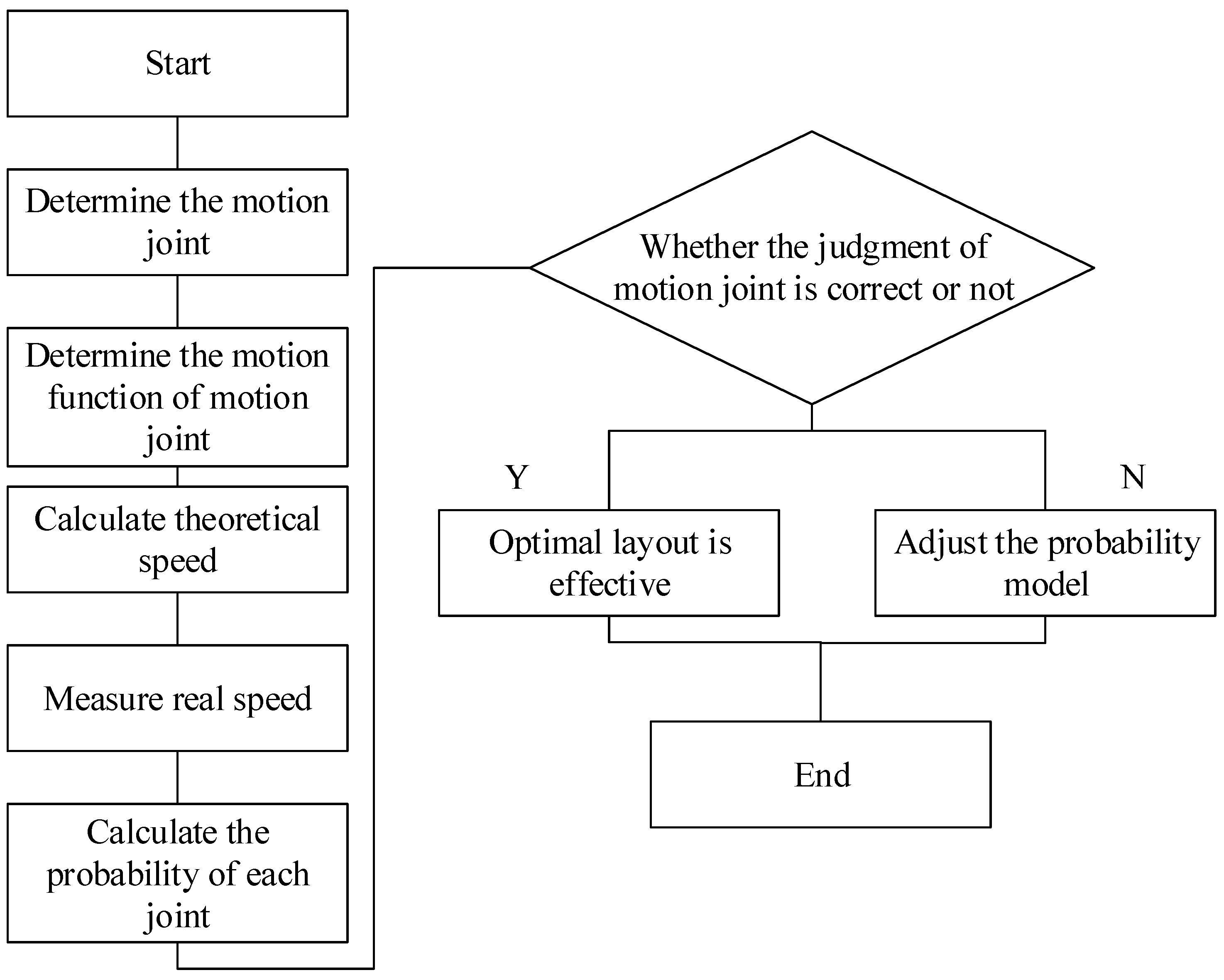
3.1. Verification Method for Layout

Because the sensor layout of an industrial robot has not formed a complete theoretical system, the judgment basis of the sensor layout should be given according to the above probabilistic method. The flow chart of the layout verification method is shown in Figure 4.
  • According to the given initial position, sensors are arranged in the corresponding position of the real industrial robot;
  • Set the joint speed of the industrial robot as a fixed speed, make the industrial robot move accordingly, and collect the acceleration of sensor distribution in the process of motion;
  • The acceleration signal is processed to get the velocity of each point, and the probability of motion from each joint is calculated by using the probability model;
  • Compare the probability of each joint with the real motion joint to determine whether the maximum probability corresponds to the real motion joint. If so, it is considered that the sensor layout can obtain the whole machine state.
In this paper, two types of experiments are conducted for industrial robots with and without models, and each type of experiment acquires a series of measured experimental data through multi-channel sensors and calculates the data pre-processing and sensor optimization layout through MATLAB for the measured experimental data. Algorithm 1 is the pseudo code for the sensor-optimized layout algorithm.
Algorithm 1: Optimal sensor placement based on Bayesian and Constraint equation
Input: the measured velocity V t and the predicted velocity V ' ( r ; s ) of the sensor.
Output: optimal sensor placement s_best.
1rn = 3;
2if sn = 1 do
3for i = 1 to rn do
4  for j = 1 to le do
5   compute p(i,j);//according to Equation (16).
6  end
7end
8for i = 1 to rn do
9  for j = 1 to le do
10   compute U(i,j);//according to Equation (19)
11  end
12end
13for i = 1 to rn do
14  compute Us(i);//sum U(i,j)
15end
16 s_best = s(max(Us));
17else
18 sn = sn + 1;
19for i = 1 to rn do
20  for j = 1 to le do
21   compute p(i,j);//according to Equation (16)
22  end
23end
24for i = 1 to rn do
25  for j = 1 to le do
26   compute U(i,j);//according to Equation (19)
27  end
28end
29for i = 1 to rn do
30  compute Us(i);//sum U(i,j)
31end
32 s_best = snew(max(Us));
33for i = 1 to rn do
34  compute n_best;//according to Equation (21)
35end
36 s_best = s_best(n_best);//optimal sensor placement
37end
38//rn—number of joints;
39//s—initial Sensor placement;
40//sn—number of sensors currently optimized;
41//le—number of sensors in the initial layout;
42//p(i j)—the likelihood function;
43//U(i,j)—the sensor placement evaluation function according to Equation (19);
44//Us(i)—sum of regression values of each sensor coordinate;
45//snew—the new sensor placement based on heuristic sequential sensor placement;
46//n_best—the optimal number of sensors according to the change of the objective function;

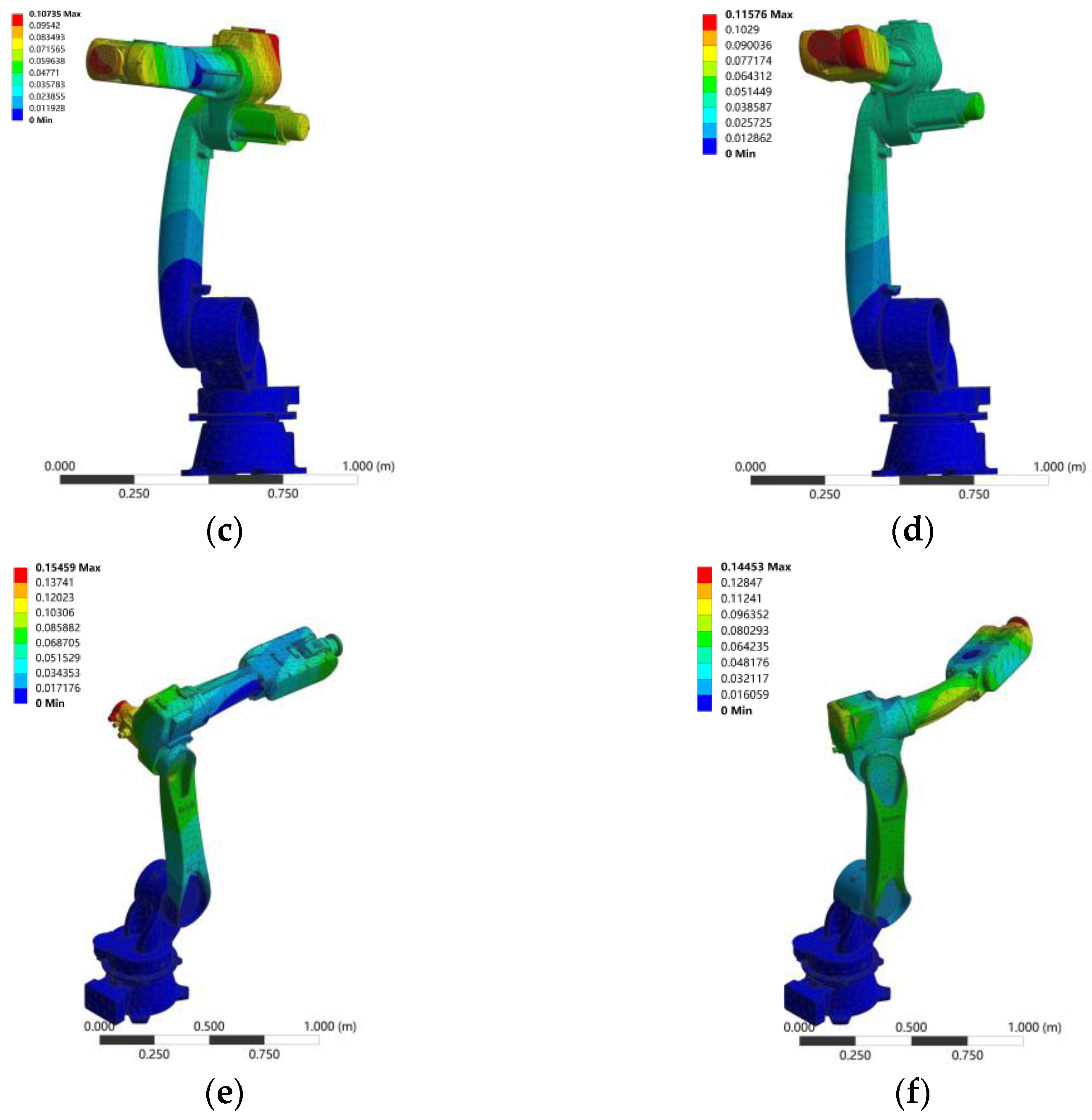
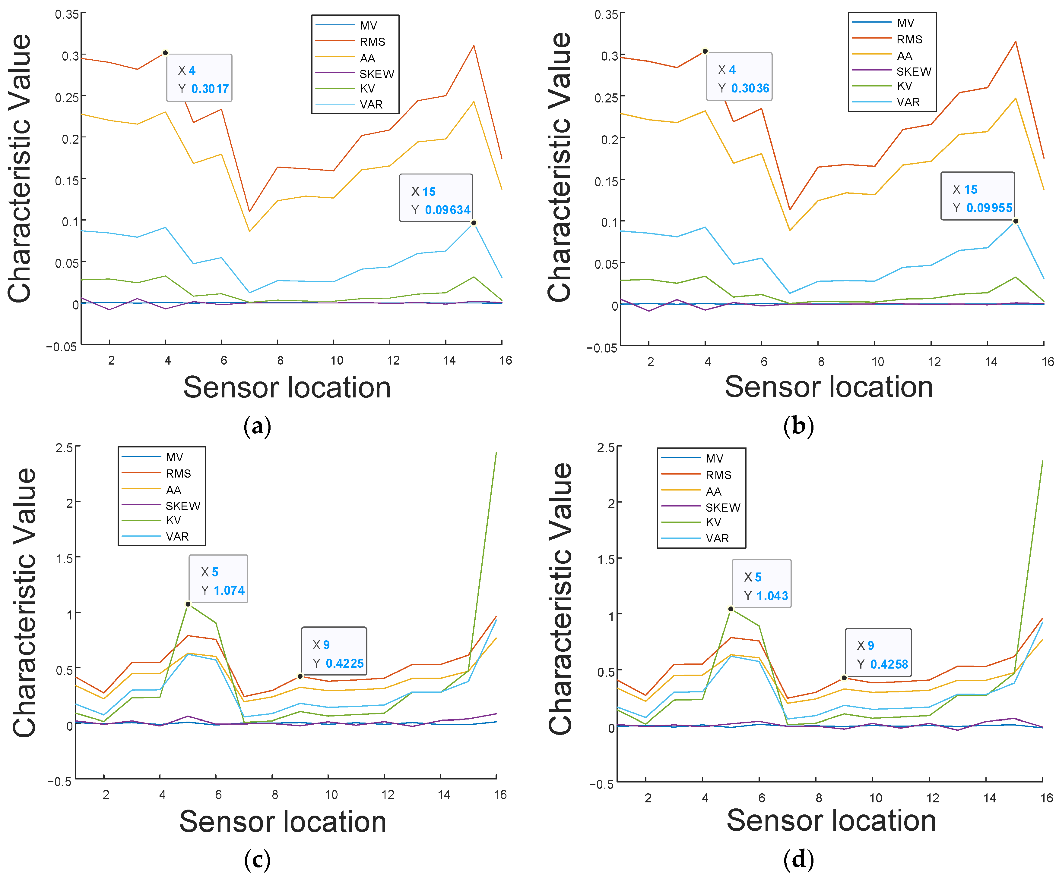
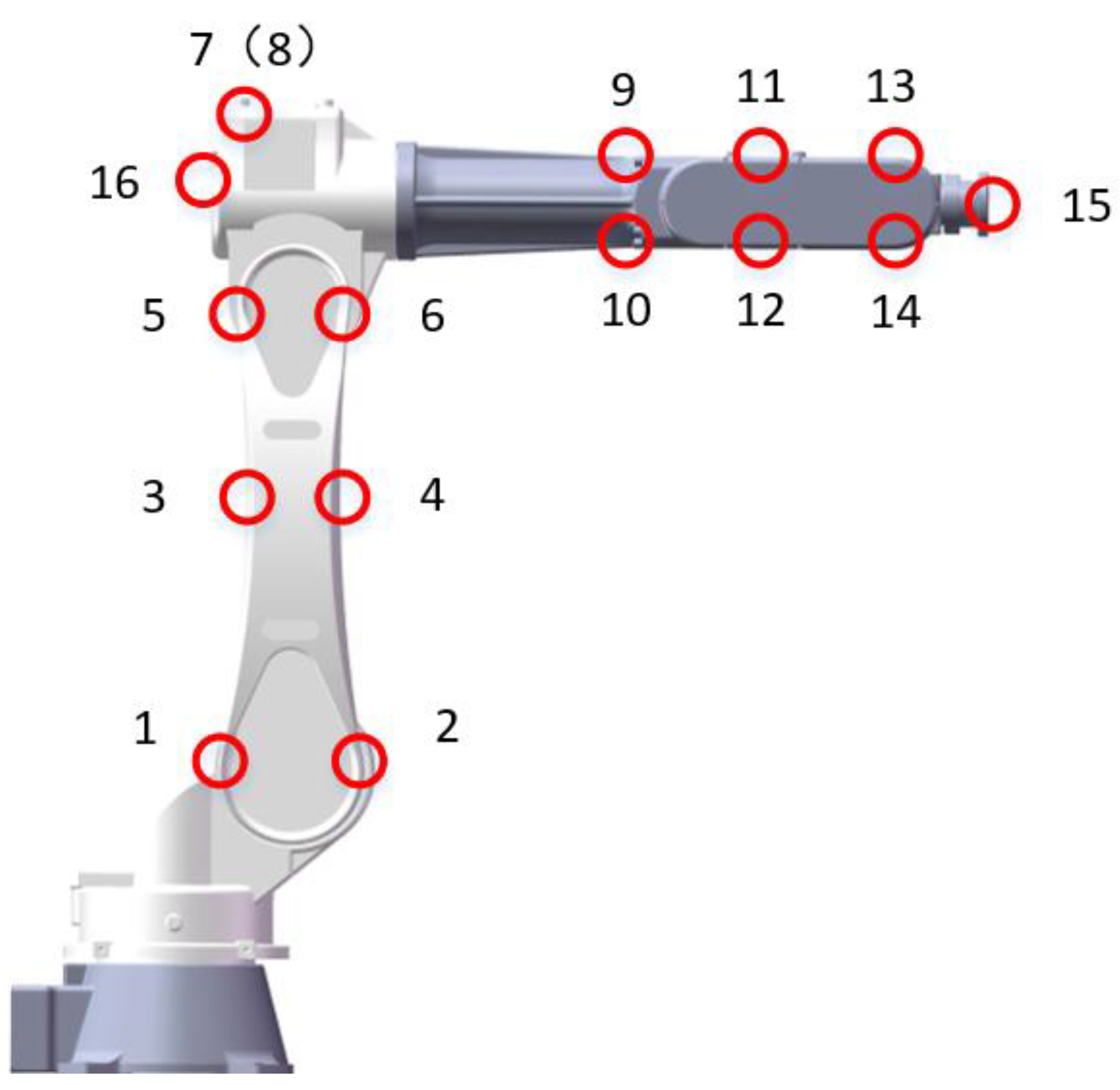
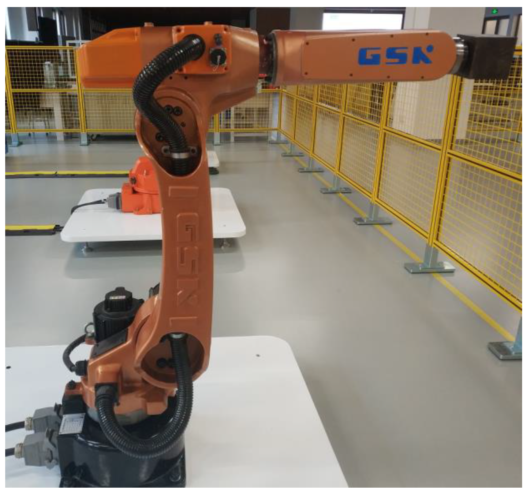
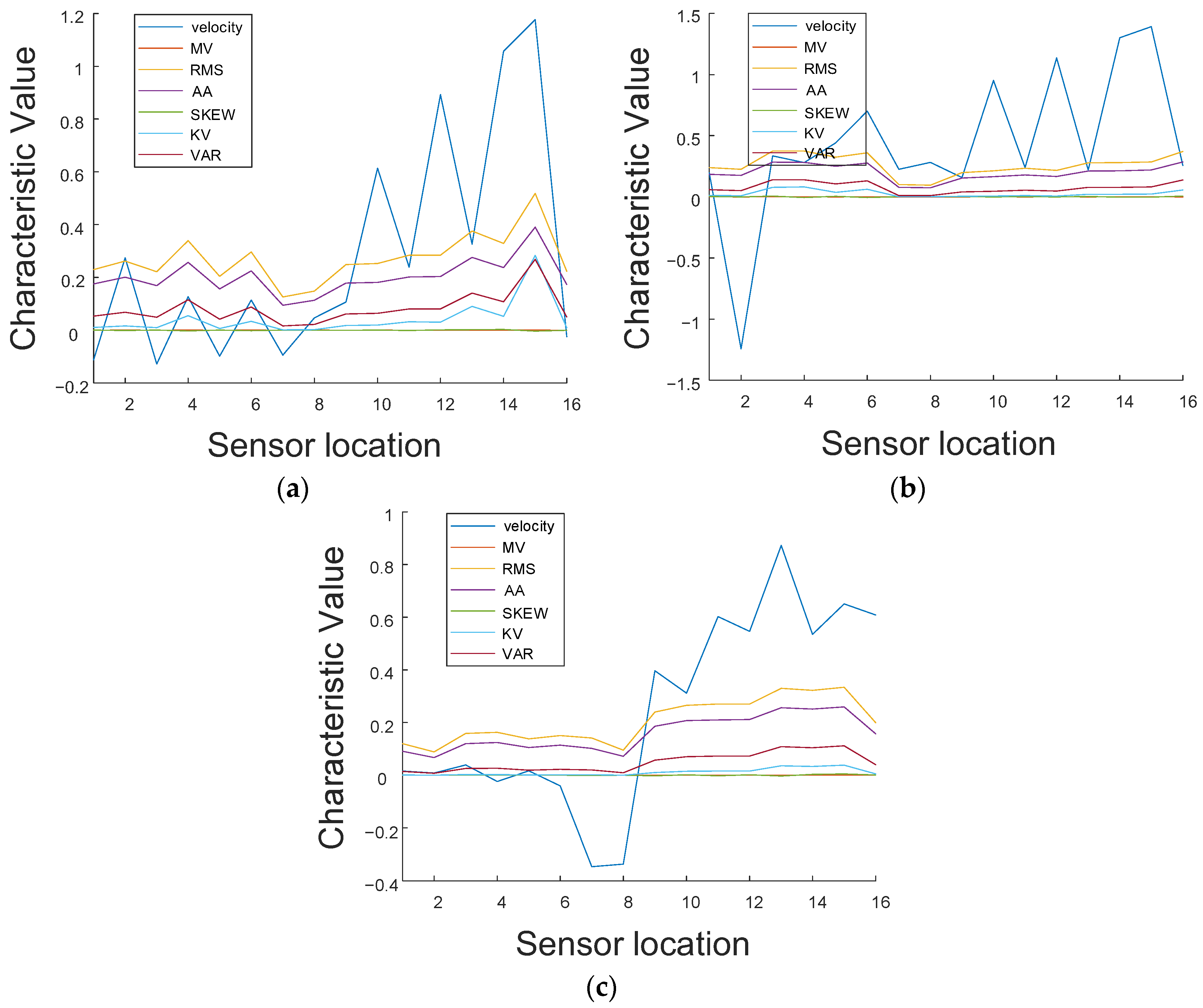
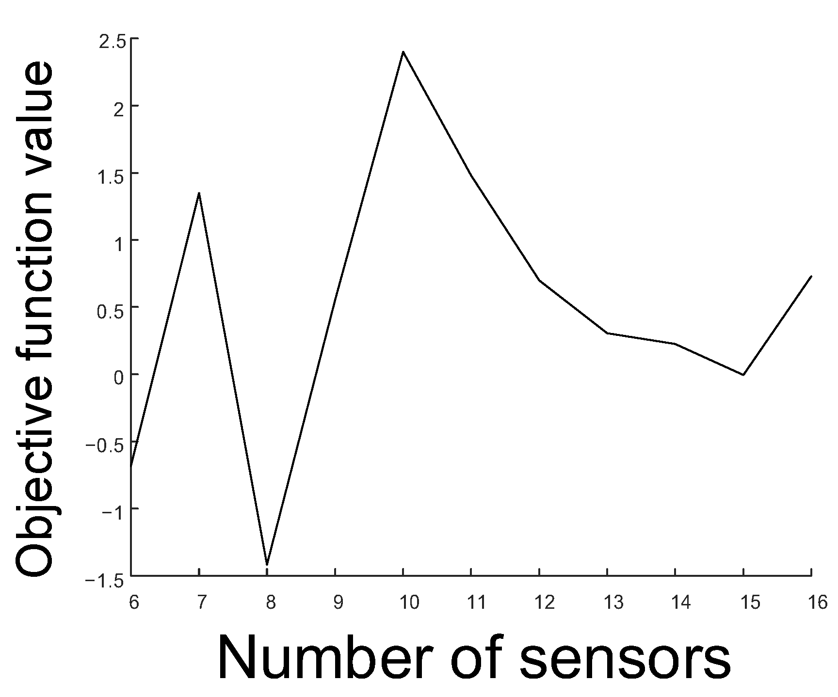
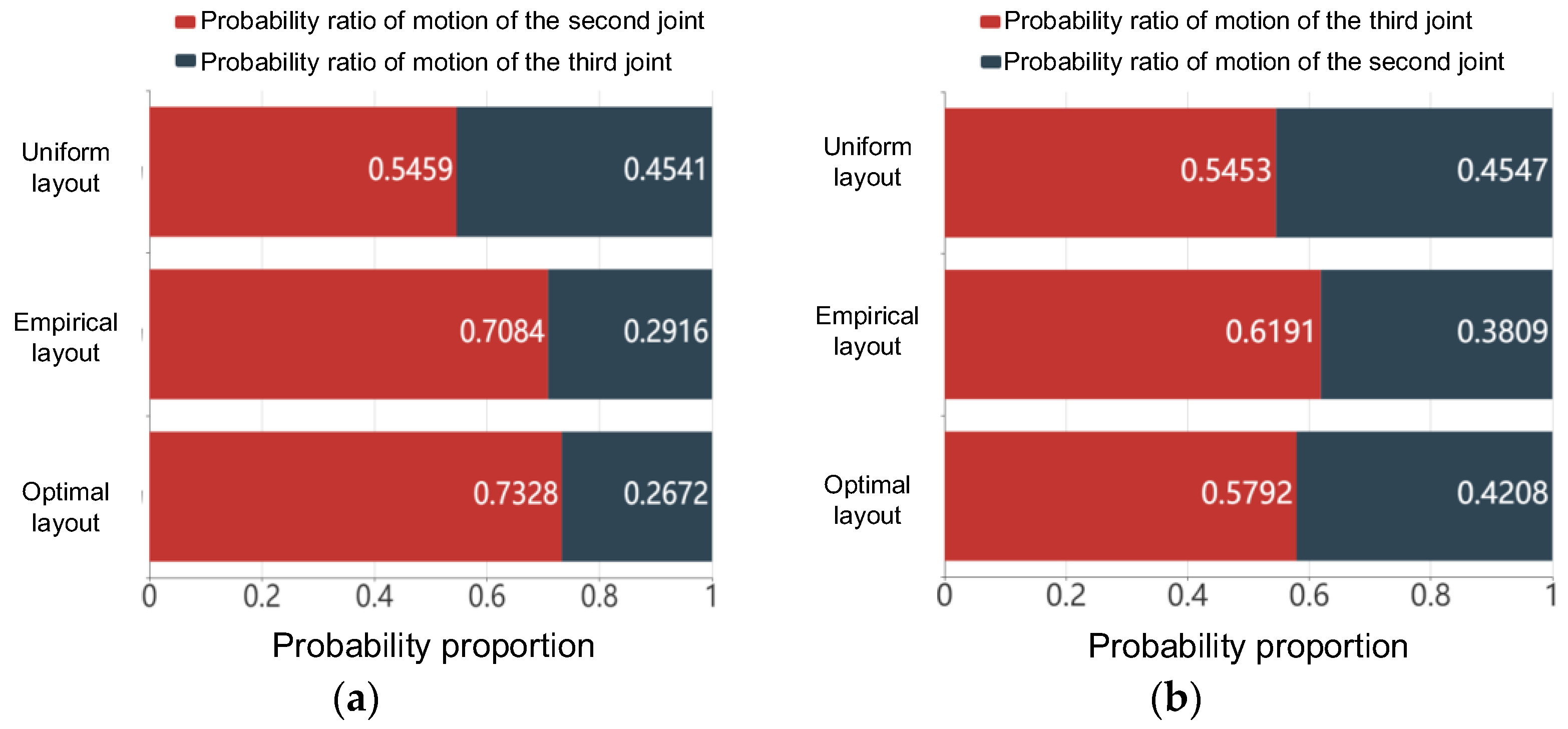
3.2. Verification of Optimal Sensor Placement for Industrial Robots Based on the Simulation Model

To verify the effectiveness of the sensor placement method proposed in this paper, we carry out a single joint motion verification experiment for a six-axis industrial robot. The experimental scene is shown in Figure 5.
To obtain the real speed, we combined the measured acceleration with the theoretical speed as noise. Moreover, because the frequency of the real collected signal is generally high, it is not advisable to reduce all acceleration points to one dimension. At the same time, bringing all acceleration points into the calculation will lead to too much calculation. Therefore, an appropriate dimension reduction method is needed to process the original signal. Considering the signal preprocessing method of the vibration signal, we select the typical time-domain characteristics of the vibration signal. The time-domain characteristics of the input vibration signal are taken as the input of the probability model for calculation. The selected features should reflect the amplitude and fluctuation characteristics of the signal. Therefore, the selected time-domain characteristics include mean value, root mean square value, absolute mean value, skewness, kurtosis, and variance. Divide the above-mentioned original signals into two groups, take 40,000 sampling points for each group of original signals, calculate the time domain signal characteristics of the two groups of signals, respectively, and combine the real speed with the time domain characteristics’ overall input. The input is shown in Figure 6.
The signal features of the three joints in motion are input into the probability model program. The optimal layout evaluation is calculated circularly, and the corresponding redundancy is calculated. The optimal layout order is [0.7, 1.47, 0.7, 0.8, 1.18, 0.8, 1.56, 1.47, 1.37, 1.37, 1.18, 0.8, 0.5, 0.5, 0.2, 0.2].
By observing the distribution of objective function values, as shown in Figure 7, and considering the problem of the degree of freedom of the industrial robot, ten sensors are selected to be arranged. The optimal sensor layout is [0.7, 1.47, 0.7, 0.8, 1.18, 0.8, 1.56, 1.47, 1.37, 1.37]. The corresponding objective function value is 2.4. The empirical layout and uniform layout are shown in Figure 8.
According to the process shown in Section 3.1, the second and third joint motions are judged by probability, respectively, and the optimal layout, empirical layout, and uniform layout are selected for comparison.
According to the results in Figure 9, in the layout verification experiment with the simulation model, the empirical layout and the optimal layout have a higher discrimination effect. In the judgment results of the third joint motion, the empirical layout shows a better discrimination effect than the optimal layout. In general, both empirical layout and optimal layout have good performance in the layout verification experiment with the model. However, due to the complex process of model simulation and kinematic analysis, this method cannot be applied to large-scale industrial scenes.

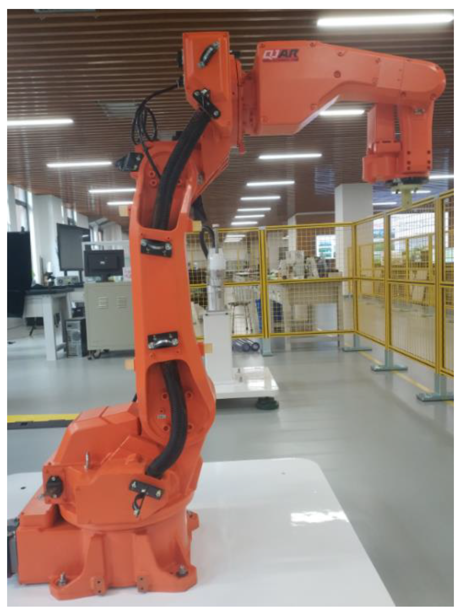
3.3. Optimal Sensor Placement Method and Verification of Industrial Robots without Simulation Models
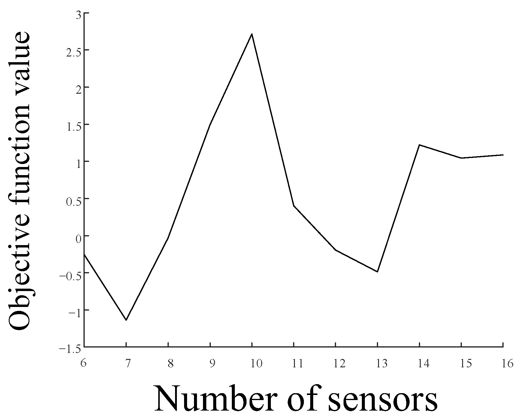
In the implementation process of the sensor layout optimization method, first, the kinematics and dynamics simulation analyses are carried out based on the simulation model and DH parameters, and the theoretical speed is taken as the theoretical value of the probability model. The subsequent optimization is carried out through the error distribution. However, in the actual scene, in some cases, the simulation model of the industrial robot is not easy to obtain, and the calculation process based on simulation analysis is more complex, which is not suitable for the scene that needs to conclude sensor placement quickly. Therefore, based on the defects of the above placement method, a sensor-optimal placement method that discards the simulation model is considered.
Considering that the calculation of theoretical velocity is due to the quantization of the error distribution in the new layout method, the acceleration signal collected by the sensor is directly taken as the real value. Because of the uniform motion of each joint, the theoretical acceleration value of each layout point is 0, so the error of the two is the real acceleration signal collected by the sensor. According to the maximum entropy principle, the acceleration signal collected by the sensor includes the interference of the theoretical acceleration value with the environmental noise and its structure, in which the environmental noise and its structure interference can be regarded as random variables; that is, the error also conforms to the multivariate Gaussian distribution. Hence, the subsequent optimization process is the same as above. The industrial robot without the 3D model used in the experiment is also a six-axis industrial robot, as shown in Figure 10.
Divide the original signals into two groups, take 40,000 sampling points for each group of original signals, and calculate the time-domain signal characteristics of the two groups of signals. The results are shown in Figure 11.
The signal features of the three joints in motion are input into the probability model program. The optimal layout evaluation is calculated circularly, and the corresponding redundancy is calculated. The optimal layout order is [1.56, 1.37, 1.18, 0.8, 0.8, 1.47, 0.7, 1.18, 0.8, 1.37, 0.2, 1.47, 0.7, 0.5, 0.5, 0.2].
By observing the distribution of objective function values, as shown in Figure 12, and considering the problem of the degree of freedom of the industrial robot, ten sensors are selected to be arranged. The optimal sensor layout is [1.56, 1.37, 1.18, 0.8, 0.8, 1.47, 0.7, 1.18, 0.8, 1.37]. The corresponding objective function value is 2.716. The empirical layout and uniform layout are shown in Figure 13.
According to the process shown in Section 3.1, the second and third joint motions are judged by probability, respectively, and the optimal layout, empirical layout, and uniform layout are selected for comparison.
According to the results in Figure 14, the uniform layout and the optimal layout have an excellent distinguishing effect, and the empirical layout has a high distinguishing effect. According to the maximum entropy principle, when the peak power is limited, the random variable with a finite domain has maximum entropy when it is uniformly distributed. Therefore, uniform distribution has a good effect when the simulation model is unknown. In general, for the layout verification experiment without a simulation model, the optimal layout still has obvious advantages. Considering the calculation process of optimal placement, we take the acquisition of joint state signal as an important basis. The objective function of optimization is quantified by relative entropy so that the optimal placement can effectively obtain the motion state of the robot.

3.4. Result

In the experiment of this paper, a verification experiment of the optimal layout method of an industrial robot sensor is completed. According to the connection of the joint motion of the industrial robot, the sensor layout verification method of the industrial robot is first designed, and the probability of each joint is considered to be compared with the real moving joint to determine whether the maximum probability corresponds to the real moving joint, and joint 2 and joint 3 are determined as the judgment kinematic joints (two joints move in the same plane). For an industrial robot with a simulation model, its optimal layout is obtained, and the optimal layout, empirical layout, and uniform layout are used to verify the layout of the industrial robot sensors. It is calculated that the optimal layout has a probability increase of 0.0244 and a probability decrease of 0.0399 compared with the empirical layout, respectively. A relatively uniform layout has a probability increase of 0.1869 and 0.0339, respectively. For the model-free simulated industrial robot, its optimal layout is obtained. Compared with the empirical layout, the optimal layout has a probability increase of 0.2693 and 0.2630, respectively, and a probability increase of 0.0277 and 0.0255, respectively, compared to the uniform layout. Based on the above experimental conclusions, the effectiveness of the optimal layout method for industrial robot sensors can be proved, and the applicability of the method in the industrial field is proved.

4. Conclusions

This paper studies the optimal placement method of sensors to obtain better data sources for the health assessment and fault diagnosis of industrial robots. The work in this paper can be summarized as follows.
Combining the 6-DOF industrial robot speed calculation formula with Bayesian optimization, taking redundancy as the constraint, and finally determining the layout method of the industrial robot acceleration sensor. Considering the importance of joint motion state information for the health assessment and fault diagnosis of industrial robots, we want this layout method to capture joint motion state information to the greatest extent. To obtain the initial sensor layout, we carry out the modal simulation of the industrial robot model. At the same time, considering the need to calculate the speed of specific points, the original speed transfer formula of the robot is rewritten, and the speed calculation formula of specific points is obtained. Considering that the evaluation function cannot give the number of sensors, the modal confidence matrix is improved by using the kinematic characteristics of the industrial robot, and the improved modal confidence matrix is used to constrain the evaluation function.
For different experimental objects, verification experiments with models and without models are carried out. Compared with the current common layout and uniform layout, the optimized layout obtained by this method can capture joint state information more effectively. The effectiveness of the optimal layout is verified by a model-based sensor optimal layout experiment, which verifies the effectiveness of the optimization method. The sensor optimal layout experiment realizes the extension of the layout method without a model. It is also proved that the optimal layout of the sensor depends on the structure of the industrial robot itself and the real signal collected by the sensor. The layout is evaluated by the error between the real signal collected by the sensor and the theoretical calculation value, and redundancy is taken as the constraint function of the layout by using part of the results of the modal simulation. Finally, the optimal layout objective function of the industrial robot acceleration sensor is obtained, which can provide better data sources for health assessment and fault diagnosis of industrial robots.

Author Contributions

Conceptualization, Q.H. and Y.Z.; methodology, Q.H., Y.Z. and Y.L.; software, Y.Z., X.X. and L.S.; validation, Q.H., Y.Z. and X.X.; formal analysis, Q.H. and Y.Z.; investigation, Y.Z. and X.Y.; resources, Q.H. and Y.Z.; data curation, Q.H. and Y.Z.; writing—original draft preparation, Q.H., Y.Z. and X.X.; writing—review and editing, Q.H., W.S., X.X., Y.L. and L.S.; visualization, Y.Z. and X.Y.; supervision, Q.H. and W.S.; project administration, Q.H. and W.S.; funding acquisition, Q.H. All authors have read and agreed to the published version of the manuscript.

Funding

This work was funded by the National Key R&D Program of China under grant 2018YFB1306101.

Institutional Review Board Statement

Not applicable.

Informed Consent Statement

Not applicable.

Data Availability Statement

Not applicable.

Acknowledgments

The authors gratefully acknowledge the financial support offered by the National Key R&D Program of China under grant 2018YFB1306101.

Conflicts of Interest

The authors declare no conflict of interest.

References

  1. Han, H.; Lin, Y.; Gu, L.; Xu, Y.; Gu, F. Vibration Analysis Based Condition Monitoring for Industrial Robots. In IncoME-V 2020: Proceedings of IncoME-V & CEPE Net-2020; Zhen, D., Wang, D., Wang, T., Wang, H., Huang, B., Sinha, J.K., Ball, A.D., Eds.; Mechanisms and Machine Science; Springer International Publishing: Cham, Switzerland, 2021; Volume 105, pp. 186–195. ISBN 978-3-030-75792-2. [Google Scholar]
  2. Xue, B. Remote Infrared Monitoring Method for Faults of Indoor Patrol Robot in Substation. In Proceedings of the 2021 7th International Symposium on Mechatronics and Industrial Informatics (ISMII), Zhuhai, China, 22–24 January 2021; pp. 24–27. [Google Scholar]
  3. Hou, Z.; Chen, J. Research Review of Remote Monitoring and Fault Diagnosis of Industrial Robots. Mach. Tool Hydraul. 2018, 46, 168, 172–176. [Google Scholar]
  4. Mi, Y.; Xu, F.; Tan, J.; Wang, X.; Liang, B. Fault-Tolerant Control of a 2-DOF Robot Manipulator Using Multi-Sensor Switching Strategy. In Proceedings of the 2017 36th Chinese Control Conference (CCC), Dalian, China, 26–28 July 2017; pp. 7307–7314. [Google Scholar]
  5. Neyens, G.; Zampunieris, D. Proactive Middleware for Fault Detection and Advanced Conflict Handling in Sensor Fusion. In Artificial Intelligence and Soft Computing; Rutkowski, L., Scherer, R., Korytkowski, M., Pedrycz, W., Tadeusiewicz, R., Zurada, J.M., Eds.; Lecture Notes in Computer Science; Springer International Publishing: Cham, Switzerland, 2019; Volume 11509, pp. 643–653. ISBN 978-3-030-20914-8. [Google Scholar]
  6. Zhou, Y.; Luo, J.; Wang, M. Dynamic Manipulability Analysis of Multi-Arm Space Robot. Robotica 2021, 39, 23–41. [Google Scholar] [CrossRef]
  7. Xu, P.; Cheung, C.-F.; Li, B.; Ho, L.-T.; Zhang, J.-F. Kinematics Analysis of a Hybrid Manipulator for Computer Controlled Ultra-Precision Freeform Polishing. Robot. Comput. Integr. Manuf. 2017, 44, 44–56. [Google Scholar] [CrossRef]
  8. Erkaya, S. Effects of Joint Clearance on the Motion Accuracy of Robotic Manipulators. Stroj. Vestn./J. Mech. Eng. 2018, 64, 82–94. [Google Scholar] [CrossRef]
  9. Yang, J.; Zhang, G.; Wang, L.; Wang, J.; Wang, H. Multi-Degree-of-Freedom Joint Nonlinear Motion Control with Considering the Friction Effect. In Proceedings of the 2021 IEEE 19th World Symposium on Applied Machine Intelligence and Informatics (SAMI), Herl’any, Slovakia, 21 January 2021; pp. 000211–000216. [Google Scholar]
  10. Long, J.; Mou, J.; Zhang, L.; Zhang, S.; Li, C. Attitude Data-Based Deep Hybrid Learning Architecture for Intelligent Fault Diagnosis of Multi-Joint Industrial Robots. J. Manuf. Syst. 2021, 61, 736–745. [Google Scholar] [CrossRef]
  11. Zhang, J.; Maes, K.; De Roeck, G.; Reynders, E.; Papadimitriou, C.; Lombaert, G. Optimal Sensor Placement for Multi-Setup Modal Analysis of Structures. J. Sound Vib. 2017, 401, 214–232. [Google Scholar] [CrossRef]
  12. Gao, Q.; Cui, K.; Li, J.; Guo, B.; Liu, Y. Optimal Layout of Sensors in Large-Span Cable-Stayed Bridges Subjected to Moving Vehicular Loads. Int. J. Distrib. Sens. Netw. 2020, 16, 155014771989937. [Google Scholar] [CrossRef] [Green Version]
  13. Zhang, X.-H.; Xu, Y.-L.; Zhu, S.; Zhan, S. Dual-Type Sensor Placement for Multi-Scale Response Reconstruction. Mechatronics 2014, 24, 376–384. [Google Scholar] [CrossRef]
  14. Yi, T.; Zhang, X.; Li, H.-N. Modified Monkey Algorithm and Its Application to the Optimal Sensor Placement. Appl. Mech. Mater. 2012, 178–181, 2699–2702. [Google Scholar] [CrossRef]
  15. Hanis, T.; Hromcik, M. Optimal Sensors Placement and Spillover Suppression. Mech. Syst. Signal Process. 2012, 28, 367–378. [Google Scholar] [CrossRef]
  16. Castro-Triguero, R.; Murugan, S.; Gallego, R.; Friswell, M.I. Robustness of Optimal Sensor Placement under Parametric Uncertainty. Mech. Syst. Signal Process. 2013, 41, 268–287. [Google Scholar] [CrossRef]
  17. Li, D.S.; Li, H.N.; Fritzen, C.P. The Connection between Effective Independence and Modal Kinetic Energy Methods for Sensor Placement. J. Sound Vib. 2007, 305, 945–955. [Google Scholar] [CrossRef]
  18. Kammer, D.C. Sensor Placement for On-Orbit Modal Identification and Correlation of Large Space Structures. In Proceedings of the 1990 American Control Conference, San Diego, CA, USA, 23–25 May 1990; pp. 2984–2990. [Google Scholar]
  19. Li, D.-S.; Li, H.-N.; Fritzen, C.-P. Load Dependent Sensor Placement Method: Theory and Experimental Validation. Mech. Syst. Signal Process. 2012, 31, 217–227. [Google Scholar] [CrossRef]
  20. Brehm, M.; Zabel, V.; Bucher, C. Optimal Reference Sensor Positions Using Output-Only Vibration Test Data. Mech. Syst. Signal Process. 2013, 41, 196–225. [Google Scholar] [CrossRef]
  21. Moreno-Salinas, D.; Pascoal, A.; Aranda, J. Optimal Sensor Placement for Acoustic Underwater Target Positioning With Range-Only Measurements. IEEE J. Ocean. Eng. 2016, 41, 620–643. [Google Scholar] [CrossRef]
  22. Flynn, E.B.; Todd, M.D. A Bayesian Approach to Optimal Sensor Placement for Structural Health Monitoring with Application to Active Sensing. Mech. Syst. Signal Process. 2010, 24, 891–903. [Google Scholar] [CrossRef]
  23. Papadimitriou, C.; Lombaert, G. The Effect of Prediction Error Correlation on Optimal Sensor Placement in Structural Dynamics. Mech. Syst. Signal Process 2012, 28, 105–127. [Google Scholar] [CrossRef]
  24. Sun, H.; Büyüköztürk, O. Optimal Sensor Placement in Structural Health Monitoring Using Discrete Optimization. Smart Mater. Struct. 2015, 24, 125034. [Google Scholar] [CrossRef]
  25. Vincenzi, L.; Simonini, L. Influence of Model Errors in Optimal Sensor Placement. J. Sound Vib. 2017, 389, 119–133. [Google Scholar] [CrossRef]
  26. Huan, X.; Marzouk, Y.M. Simulation-Based Optimal Bayesian Experimental Design for Nonlinear Systems. J. Comput. Phys. 2013, 232, 288–317. [Google Scholar] [CrossRef] [Green Version]
Figure 1. Industrial robot connecting rod coordinate system.
Applsci 12 06086 g001
Figure 2. The first six modes of industrial robot: (a) 1st order mode shape, (b) 2nd order mode shape, (c) 3rd order mode shape, (d) 4th order mode shape, (e) 5th order mode shape, and (f) 6th order mode shape.
Applsci 12 06086 g002aApplsci 12 06086 g002b
Figure 3. Selection of initial sensor placement.
Applsci 12 06086 g003
Figure 4. Flow chart of the layout verification method.
Applsci 12 06086 g004
Figure 5. Industrial robot with the simulation model.
Applsci 12 06086 g005
Figure 6. Data characteristics of motion data: (a) data characteristics of the first joint, (b) data characteristics of the second joint, and (c) data characteristics of the third joint.
Applsci 12 06086 g006
Figure 7. Objective function value for Industrial robot with the simulation model.
Applsci 12 06086 g007
Figure 8. Three kinds of layouts for Industrial robot with the simulation model: (a) optimal layout, (b) empirical layout, and (c) uniform layout.
Applsci 12 06086 g008
Figure 9. Probabilistic verification of three layouts: (a) Probability verification of the second joint in motion, (b) Probability verification of the third joint in motion.
Applsci 12 06086 g009
Figure 10. Industrial robot without simulation model.
Applsci 12 06086 g010
Figure 11. Data characteristics of motion data: (a) data characteristics of the first half of the first joint, (b) data characteristics of the second half of the first joint, (c) data characteristics of the first half of the second joint, (d) data characteristics of the second half of the second joint, (e) data characteristics of the first half of the third joint, and (f) data characteristics of the second half of the third joint.
Applsci 12 06086 g011aApplsci 12 06086 g011b
Figure 12. Objective function value for Industrial robot without the simulation model.
Applsci 12 06086 g012
Figure 13. Three kinds of layouts for industrial robot without the simulation model: (a) optimal layout, (b) empirical layout, and (c) uniform layout.
Applsci 12 06086 g013
Figure 14. Probabilistic verification of three layouts: (a) Probability verification of the second joint movement, (b) Probability verification of the third joint in motion.
Applsci 12 06086 g014
Table 1. Method for establishing a D-H coordinate system.
Origin   o i z i - Axis x i - Axis y i - Axis
When the axis of joint i intersects with the axis of joint i + 1 , the intersection point is takenCoincides with the axis of joint i If the joint axis i intersects i + 1 , it is perpendicular to the plane where the joint axis i and i + 1 are locatedDetermined by the right-hand rule
When the axis of joint i is out of plane with the axis of joint i + 1 , take the intersection of the common perpendicular of the two axes and the axis of joint i On the common perpendicular of the links i and i + 1 , its direction is from i to i + 1
When the axis of joint i is parallel to the axis of joint i + 1 , take the intersection of the common perpendicular of the axis of joint i and the axis of joint i + 1 with the axis of joint i
Table 2. D-H parameters of industrial robots.
Link\Parameters a i 1 α i 1 d i θ i
1000 θ 1
2 a 1 π / 2 0 θ 2
3 a 2 00 θ 3
40 π / 2 d 4 θ 4
50 π / 2 0 θ 5
60 π / 2 d 6 θ 6
Table 3. Parameters of the industrial robot with the model.
ProjectTypeNumber of AxesDriving ModeRepeat Positioning AccuracyRange of Motion
ParameterRB136AC servo0.07 mmR499~R1404 mm
Table 4. The first six natural frequencies and amplitudes.
Order123456
Natural frequency/Hz12.620.030.070.3116.7338.3
Maximum relative amplitude/m0.110.090.100.120.150.14
Publisher’s Note: MDPI stays neutral with regard to jurisdictional claims in published maps and institutional affiliations.

