Price Forecast for Mexican Red Spiny Lobster (Panulirus spp.) Using Artificial Neural Networks (ANNs)

Abstract

The selling price is one of the essential variables in decision making for fishers regarding the catching of a fishing resource. In the case of the Pacific Mexican lobster fishery, the price uncertainty at the beginning of the season translates into the suboptimal utilization of this resource. This work aims to predict the export price of Mexican red lobster (Panulirus) in a fishing season using demand-related market variables including price, main competitors, main buyers, and product quantities exported/imported in the market. We used the monthly export price from 2006 to 2018 for the main importer, China. As a method for price forecasting, artificial neural networks (ANNs), with and without exogenous variables (NARX, NAR), were used as an autoregressive model, while the same information was analyzed with an ARIMAX model for comparative purposes. It was found that ANNs are a useful tool that yielded better predictive power when forecasting Mexican lobster export prices compared to ARIMAX models. The predictive power was evaluated by comparing the mean square errors (MSE) of 15 models. The MSE of ANNs (73.07) was lower than that of the four ARIMAX models (88.1). It is concluded that neural networks are a valuable tool for accurately predicting prices relative to real values, an aspect of great interest for application in fishery resource management.

1. Introduction

Catches of spiny lobsters (Panulirus spp.) in Mexico amount to 4900 tons in 2018 [1]. The prices of these catches translate to an income of approximately USD 53 million, which is an essential income for maintaining several coastal communities that depend on small-scale fisheries [2,3]. The area that mainly benefits from this resource is the western coast of the Baja California peninsula, home to the red lobster (Panulirus interruptus), a species that accounts for 66% (≈3.200 mt) of lobster catches in Mexico. Forty-eight percent of these catches are exported, mainly to China (47%) [1,4].

The average annual export prices are relatively stable, showing a steady rise from 21 USD/kg to 40 USD/kg from 2006 to 2020 [4]; on an interannual scale, however, catches tend to be highly variable. This fishery has a closed season that lasts from 1 March to 30 September [5], during which the sale and marketing of the product is strictly prohibited. It is marketed as whole live lobster.

From an economic perspective, price uncertainty translates into the suboptimal utilization of fishery resources [6,7]. For this reason, it is essential to have a reliable method of predicting future prices that will improve the decision making of resource users.

Having a forecast of the lobster export price with a monthly resolution represents basic information for the marketing strategy of fishers to accrue economic benefits through the better planning of catches during the fishing season. It is possible to implement a scheduled catch during the season for this fishery since it is managed through TURF (Territorial Use Rights for Fishing), allocated to fishing cooperatives according to minimum sizes and quotas. In the study area, this management system is characterized by effective governance, and in 2004 it was the first fishery to be certified by the Marine Stewardship Council [8].

Price forecasting can benefit resource management; however, empirically estimating future prices is a complex issue [9,10,11,12]. As the red lobster is an export product, its price is not only set according to seasonality and catch quantity in a given season but is influenced by the dynamics of international markets [13]. For this reason, price forecasting requires the use of robust analytical tools [14,15,16].

Despite the importance of price in decision making related to natural resources, there is little research on the price forecasting of fisheries’ resources. Articles related to the price forecasting of pelagic fishes using the autoregressive integrated moving average with exogenous variables (ARIMAX) as a prediction model are reported in the scientific literature [17,18,19]. These works found that ARIMAX models fit the prediction of the price pattern, but as expected, the accuracy of the algorithm decreases as the forecast period becomes longer. To overcome the predictive power limitations of ARIMAX, the application of artificial neural networks (ANNs) has been proposed, which generally yield better predictive power [20,21,22,23,24,25].

ANNs are models that seek to reproduce the behavior of the human brain using a set of artificial neurons connected to each other to transmit signals [26]. ANNs are a family of powerful algorithms with which complex behaviors can be modeled when calculating a mathematical function. A trigger function is applied to a weighted sum of input values to produce an output value. Moreover, ANNs are non-parametric approximation methods commonly used in the construction of non-linear regression models [27,28]. For non-linearity, there are univariate autoregressive neural networks (NAR) based on a single data series; for one or more exogenous variables, there are NARX, which explain the dependent variable.

ANN predictions tend to perform better than ARIMAX, as ANNs are more efficient at modeling volatility. They are able to recognize time-series patterns and non-linear characteristics, yielding a better accuracy than other models; consequently, ANNs are frequently used for prediction purposes, such as fluctuations in the monthly mean level of the surface of the Caspian Sea in the short term [29], data mining and modeling of river systems [30], estimating the daily water discharge with two input variables from rainfall stations at Langat River in Malaysia [31], predicting the daily returns of crude oil prices [32], analyzing the Singapore housing market and future condominium price index [33], measuring electrical load accurately to help power companies with better scheduling and efficient management [34], predicting human mortality rates [35], implementing preventive healthcare interventions and epidemic control [36], predicting monthly tourism demand for ten European countries [37], and tracking COVID-19 cases [38], identifying 6 mA modifications for a deep understanding of cellular processes [39] and sites of Histone lysine crotonylation (Kcr) in histone proteins [40].

In addition, Tealab et al. [41] carried out a bibliographic review of works related to the prediction of time series using artificial neural networks for the period 2006–2016, observing that the models proposed in the selected studies do not fully satisfy a procedure for building an ANN model. Meanwhile, Tran et al. [42] carried out a bibliographic review of the use of neural networks to forecast air temperature for 2005–2020 and concluded that the ANN methods are viable for short-term forecasts.

Artificial neural networks have been applied in different fields, such as (a) for solving the facial recognition problem. Meng et al. [43] used an approach using a basic function of radial classification in the training of a neural network and the results highlighted the excellent performance in terms of error with regard to classifying and efficient learning. (b) They have been applied to provide effective real-time traffic signal control for a large complex traffic network; Srinivasan et al. [44] used a hybrid NN-based multiagent system.

Various neural network models are used for price forecasting in the market using different indexes, such as the New York Stock Exchange (NYSE) [45], NASDAQ stock exchange [46], price of gold stock in the NYSE [47], real estate price in Hong Kong [48], and Apple stock in NASDAQ [49].

Despite the predictive power, the widespread use of ANNs, and the relevance of having price forecasts for decision making, no information is currently available on the application of this tool for the price forecasting of fisheries’ resources. For this reason, the objectives of this work are to (1) predict Mexican lobster prices using ANNs and (2) to compare the performance of ANNs with ARIMAX models commonly used for the price forecasting of fishery products.

2. Materials and Methods

The monthly export price of the Mexican red lobster (Panulirus interruptus) (P-R) to China was selected as the predicted variable.

2.1. Selection of Variables

External factors (exogenous variables) may influence the behavior of the export prices of Mexican lobster and other products [50]. Thus, 31 variables were selected considering the basic elements related to product demand (Mexican red lobster) in market research: price, main competitors, main buyers, and quantities of product exported/imported into the market (

Table 1. Exogenous variables affecting Mexican lobster prices. Data are monthly figures for the years 2006 to 2018 (Sources: [1,4,51]).

Variable	Abbreviation
Lobster production in Mexico	PMex
Lobster price in Australia	PAus
Export price of Mexican lobster in Hong Kong	PMexHK
Export price of Mexican lobster in the USA	PMexUsa
Export price of Mexican lobster in Taiwan	PMexTC
World export price of New Zealand lobster	PNZMun
Export price of New Zealand lobster in Hong Kong	PNZHK
Export price of New Zealand lobster in the USA	PNZUsa
Export price of New Zealand lobster in Taiwan	PNZTC
World export price of Australian lobster	PAusMun
Export price of Australian lobster in Hong Kong	PAusHK
Export price of Australian lobster in the USA	PAusUSA
Export price of Australian lobster in Taiwan	PAusTC
Price Increase of Australian lobster	VCAus
Price increase of New Zealand lobster	VCNZ
Price Increase of Mexican lobster	VCMex
Export volume of Mexican lobster in Hong Kong	VMexHK
Export volume of Mexican lobster in Taiwan	VMexTC
Export volume of Mexican lobster in USA	VMexUSA
Export volume of Australian lobster in Hong Kong	VAusHK
Export volume of Australian lobster in Taiwan	VAusTC
World export volume of Australian lobster	VAusMun
Export volume of Australian lobster in USA	VAusUsa
Volume of lobster imported to the USA from Australia	VUSAAus
Volume of lobster imported to the USA from Mexico	VUSAMex
Volume of lobster imported to the USA from New Zealand	VUsaNZ
Volume of lobster imported to Taiwan from Australia	VTCAus
Volume of lobster imported to Taiwan from Mexico	VTCMex
Volume of lobster imported to Taiwan from New Zealand	VTCNZ
Apparent domestic lobster consumption in Mexico	CNA
Per capita lobster consumption in Mexico	CPCMex

).

To identify the variables with the greatest effect on Mexican lobster export price (the target variable), a correlation matrix was built with the 31 exogenous variables; subsequently, those with a higher simple linear correlation coefficient were selected using the Spearman coefficient (rho). This method was used because it allows us to measure the correlation for data that are not normally distributed [52].

Once the predictive variables were selected, the time series of export prices from Mexico to China (Hong Kong) were built using two models that accept dynamic inputs: (1) a non-linear autoregressive network (NAR) and (2) an autoregressive network with exogenous inputs (NARX). In the latter, the model was used for one, two, three, and four exogenous variables, selected for their high correlation.

ANNs were used as an autoregressive model to forecast prices, with the ARIMAX model used for comparative performance purposes.

2.2. Model Development

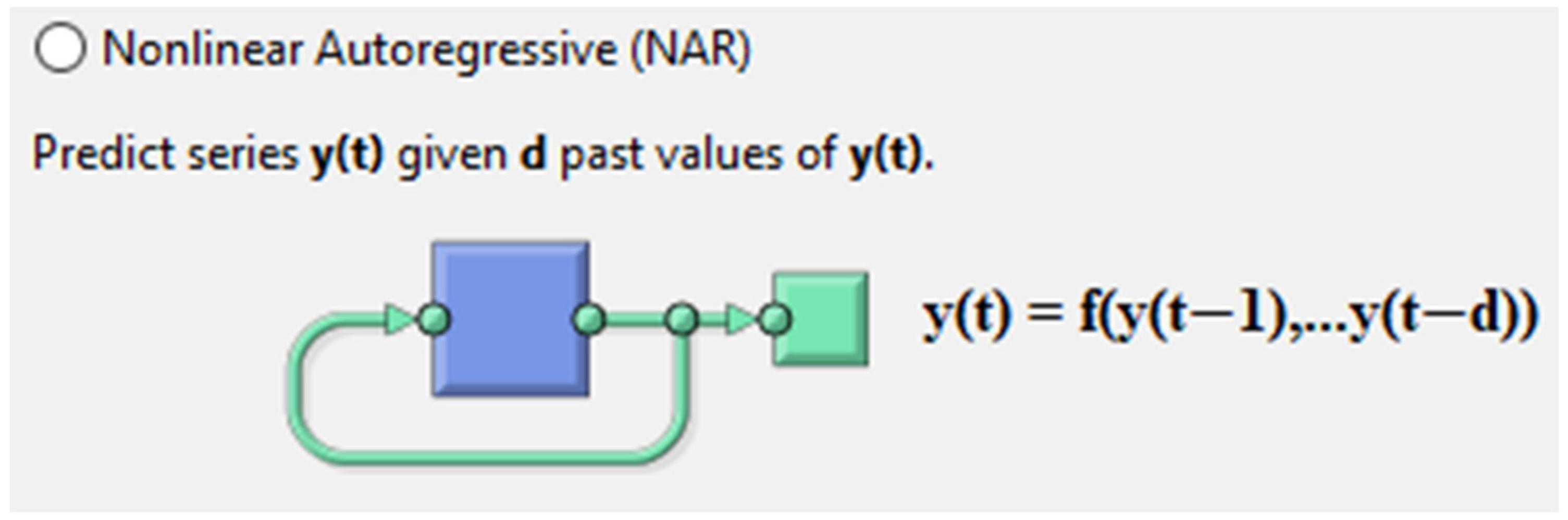
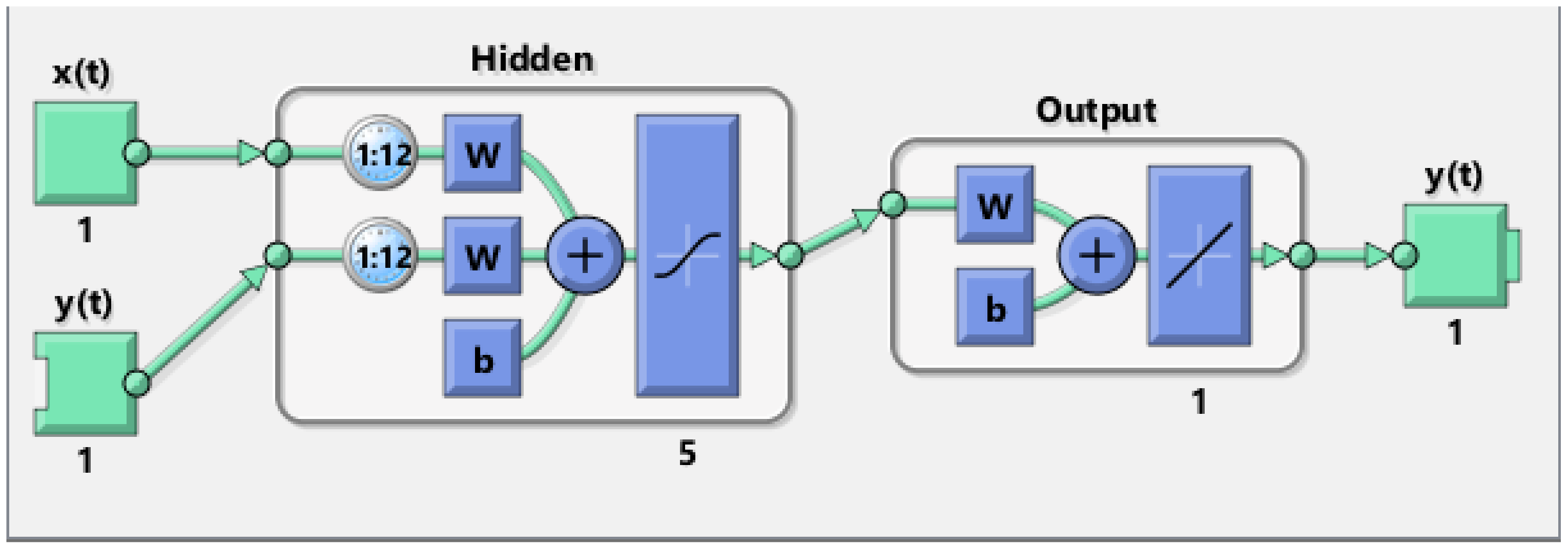
2.2.1. Neural Networks

Two typical models of neural networks with an input layer, a hidden layer (transfer function), and an output layer were used. Representations of both architectures are shown in Figure 1 and Figure 2.

NAR is a non-linear autoregressive neural model based on a single data series that functions as an input and output. This model predicts the values of the series using only past observations of the series to be predicted (target variable) [53].

Autoregressive models with exogenous variables (ARX) are mathematical tools that weigh the inputs to the system through linear filters. These models have many advantages in their estimation and predictive use because optimal predictors are always stable [54].

NARX is based on this ARX model and is a repetitive dynamic system. It is also a non-linear autoregressive model with exogenous variables, i.e., one of the variables that explain it is a dependent variable [55].

NARX networks with the gradient descent learning algorithm were applied as they offer several significant advantages: first, learning is more effective in NARX than in traditional neural networks; second, convergence is more accurate and faster in NARX than in other networks [56].

In artificial neural networks, models are obtained by trial and error. This implies that there is no specific procedure to obtain the best network. In this sense, the procedure starts from an initial network and by testing several training algorithms a final network that meets the expectations is obtained [57]. Aspects such as data preparation or the training technique used play a central role in the quality of the final model obtained; for this reason, the model construction process is a non-trivial task [58]. The variable elements for modeling are mainly the definition of relevant inputs, delays, and hidden neurons (hidden layers) [54].

NAR or NARX are multilayer perceptron networks, where once the series for use is available, delays (a simple way to recognize past patterns of the input variables), the number of hidden layers (number of neurons in the network), and the training algorithm (learning of the neural network to calculate the correct output) are defined [20] (Figure 3).

Input: The input layer is used to accept raw data for network processing and consists of neurons from which the input signals are sent to the hidden layer. In this study, five input signals were evaluated (four exogenous variables and the target variable). The input dataset is divided into two groups: (a) training data and (b) test data.

Hidden layer: In this layer, the effectiveness of the network is measured by the activation function. The activation function refers to the feature of activated neurons that allows them to be retained and mapped out by a non-linear function, which can be used to solve non-linear problems. The activation function is used to increase the expression ability of the neural network model, which gives the neural network a kind of artificial intelligence [59]. In this work, we used the tanh function, which is a symmetric function centered on zero. The convergence rate is higher than the common sigmoid function. The formula of the tanh function is defined as Equation (1):

$$f\left(x\right)=\frac{1-e^{-2x}}{1+e^{-2x}}$$

(1)

Output: The output layer has a number of neurons that is equal to the number of target variables. In this work, the activation function of the output layer is linear because a regression with the ANN was used.

A Bayesian training algorithm was used to determine the weights of neural network connections since this solves generalization and optimization issues, achieving convergence toward a set of optimal weights [60]. This training was developed to convert non-linear systems into “well posed” problems [60]. In general, the training step is aimed at reducing the sum squared error of the model output and target value. Bayesian regularization adds an additional term to this Equation (2):

$$F=\beta E_D+\alpha E_w$$

(2)

where F is the objective function, $E_D$ is the sum of squared errors, $E_w$ is the sum of the squares of the network weights, and $\alpha$ and $\beta$ are objective function parameters [61]. Since the weights are considered to be random variables in a Bayesian network, their density function using Bayes’ rule [62] is written as follows (3):

$$P\left(w|D,\alpha ,\beta ,M\right)=\frac{P\left(D|w,\beta ,M\right)P(w|\alpha ,M)}{P(D|\alpha ,\beta ,M)}$$

(3)

where D represents the data vector, M is the neural network model, and w is the vector of network weights.

Of the total data (132 price values corresponding to 132 months), 70% (92 price values of 132) were used for the training phase, yielding a fitness accuracy of between 85% and 98%; the remaining 30% (40 price values of 132) of the data were used for testing, obtaining an accuracy between 75% and 85%. This outcome means that the trained models achieve proper generalization and can be considered suitable (as long as the metrics obtained are deemed adequate) since the accuracy is greater than 85%.

The Bayesian regularization backpropagation algorithm for neural network training disables validation stops by default. It does not require a validation data set because the goal of checking validation is to see if the error in the validation set gets better or worse as training progresses [62,63].

The number of neurons and hidden layers was selected empirically, which allows for a compromise between its extensive structure and the correct generalization of the processed data [64]. This work evaluated different architectures, testing 1 hidden layer and 4 to 15 neurons, and defining 12 delays due to the monthly data frequency. The tests were performed using MATLAB^© (R2021a).

2.2.2. Autoregressive Integrated Moving Average with an Exogenous Variable

The ARIMAX model uses variations and regressions of statistical data to find patterns for projections into the future. This model is composed of an autoregressive (AR) submodel, an integration (I) submodel, and a moving average (MA) submodel with an exogenous variable. ARIMAX models are linear time-series models in which these series may or may not be stationary [65].

2.2.3. Comparison of ANN and ARIMAX Approach

The goodness of fit values of ANN and ARIMAX were determined using the coefficient of determination $R^2$, the mean squared error (MSE) and the mean absolute error (MAE). $R^2$ was calculated as follows (4):

$$R^2=1-\frac{\sum {\left(y_{exp}-y_{pred}\right)}^2}{\sum {\left(y_{exp}-\overline{y}\right)}^2}$$

(4)

The MSE represents the average squared difference between the predicted values estimated from a model and the actual values. The MSE is measured as follows (5):

$$\mathrm{MSE}=\frac{\sum {\left(y_{exp}-y_{pred}\right)}^2}{M}$$

(5)

where $y_{exp}$ represents experimental values, $y_{pred}$ represents predicted values, and M is the total numbers of data. When an input is entered into the network, the output (network result) is compared with the target. The MSE is then calculated to show the difference from this comparison. Therefore, the average sum of mean squared errors is expected to be low.

We also include MAE, since there are studies suggesting that the MSE is not a good indicator of average model performance and that therefore MAE is a better metric for this purpose [66,67].

MAE measures the average magnitude of absolute differences between N predicted vector $S=\left\{x_1,x_2,\dots ,x_N\right\}$ and N actual observations $S^{\ast }=\left\{y_1,y_2,\dots ,y_N\right\}$. The corresponding loss function is shown as (6):

$$\mathrm{MAE}=\frac{{{\displaystyle \sum }}_{i=1}^N\left|y_i-x_i\right|}{N}$$

(6)

where $y_i$ is the prediction and $x_i$ is the true value. This error is expected to be low, like the MSE.

The lobster export prices for the first three months of 2017 were projected using three prediction methods with data from January 2006 to December 2016: (1) a non-linear autoregressive network (NAR), (2) an autoregressive network with exogenous inputs (NARX for one, two, three, and four selected exogenous variables), and (3) an integrated autoregressive moving average model (ARIMAX) with and without an exogenous input variable. The ARIMAX model was used only to compare its prediction accuracy versus the other models since it is the model most commonly used for estimating price forecasts of marine resources [68,69,70]. The MSE value of each model was used to calculate the goodness of fit of the forecast.

The monthly prices database (real, Arimax and NARX best fit exogenous variables) is shown in the Supplementary Materials (Supplementary Material Table S1).

3. Results

The set of exogenous variables considered in the present study and their correlations with the target variable (Supplementary Material Table S2) clearly indicate that lobster production in Mexico (PMex), the world export price of the Australian lobster (PAusMun), the export volume of lobster to Hong Kong from Mexico (VMexHK), and the apparent domestic lobster consumption in Mexico (CNAMex) yielded the highest correlations with the Mexican lobster export price (

Table 2. Correlation between the export price of Mexican lobster to China (dependent variable) and the selected exogenous variables.

Export Price from Mexico to Hong Kong
Selected Exogenous Variables	Correlation (rho)
PMex	0.51
PAusMun	0.46
VMexHK	0.86
CNAMex	0.41

).

The historical monthly series of these exogenous variables for the selected period (January 2006 to December 2016) is shown in Figure 4.

Using Bayesian optimization with five hidden layers and 12 delays resulted in a high R² value (>0.80).

Table 3. Goodness of fit (R²) of the NAR and NARX models with the exogenous variables selected relative to the export price of the Mexican lobster to China.

	R2		R2		R2		R2
NAR, P-R only	0.92	NARX2	0.96	NARX1	0.94	NARX3	0.95
		PAusMun		CNA		PMex
		VMexHK				PAusMun
						CNA
NARX1	0.93	NARX2	0.94	NARX2	0.96	NARX3	0.91
PMex		PAusMun		PMex		PMex
		CNA		PAus		VHK
						CNA
NARX1	0.96	NARX2	0.86	NARX2	0.93	NARX3	0.92
PAus		VMexHK		PMex		PAusMun
		CNA		VMexHK		VMexHK
						CNA
NARX1	0.91	NARX3	0.91	NARX2	0.96	NARX4	0.96
VHK		PMex		PMex		PMex
		PAusMun		CNA		VMexHK
		VMexHK				PAusMun
						CNA

shows the goodness of fit (R²) for the NAR and NARX autoregressive models with one, two, three, and four variables relative to the target variable.

The forecast of Mexican lobster export prices using the NAR, NARX, and ARIMA models for the first three months of 2017 is shown in

Table 4. Forecast of Mexican lobster export prices to China for the first three months of 2017.

		NAR	NARX
2017	P-R	P-R Only	PMex	Paus	VHK	CNA	PMex, Paus	PMex, VHK
Month 1	39	40	27	30	29	27.3	27.5	46.6
Month 2	36	29	40.7	33	31	15.6	35	22.4
Month 3	33	17	35.3	24	33	31.5	40.8	38.6
MSE		42	56	51.8	6.6	58.5	25.4	117
MAE		8	6.3	7	5	11.2	6.7	8.9
	NARX
2017	PMex, CNA	PAus, VHK	PAus, CNA	VHK, CNA	PMex, PAus, VHK	PMex, PAus, CNA	PMex, VHK, CNA
Month 1	27	27	27	27	30.5	27	30.5
Month 2	46.6	38	18.5	33	21.5	31.3	31.2
Month 3	54.2	30	44	37	61.5	42.5	44.5
MSE	228	45	54	11.3	231.8	19.4	28
MAE	14.6	5.6	13.5	6.3	17	8.7	8.2
	NARX		ARIMAX
2017	PAus, VHK, CNA	PMex, PAus, VHK, CNA	PAus	PMex	VHK	CNA
Month 1	33	27	47.4	47.8	49	48.4
Month 2	32.8	17.8	48.6	51.5	50.6	48.9
Month 3	42	53	35.3	44.21	40.24	39.26
MSE	27.8	135.5	95.6	117.8	99.5	136.1
MAE	6	16.7	7.7	11.8	10.6	9.5

.

For the validation, the MSE and MAE were measured by comparing the predicted price versus the real values (P-R). It was observed that the neural network models yielded a better accuracy, particularly NARX with the exogenous variable VMexHK and NARX with two exogenous variables (VMexHK and CNA), which yielded the lowest MSE values.

Figure 5 shows the fit of the regression for Mexican lobster export prices (month 1 to 132) with their respective closed seasons. It is important to recall that the forecast obtained with the NARX model using the exogenous variable VMexHK is only for the first three months of 2017 and the historical series of export price from January 2006 to March 2017. The validation curve between the observed data and the estimated data from NARX and ARIMAX attained a good fit ($R^2$ = 0.91).

The adjustment of the NARX regression was trained using data from January 2006 to January 2010. After this, an improvement in the precision of the adjustment was observed (February 2010 to December 2016). Therefore, the forecasted price for January, February, and March 2017 is closer to the real prices. The figure above shows how the NARX model, in addition to learning to predicted prices, also learns to identify closed seasons in which there is no catch, and so a value of 0 is assigned to the price.

The values obtained with neural models showed that these predicted values are close to the actual values, with a difference ranging between USD 0.2 and 10 for NARX with the exogenous variable VMexHK and between USD 3 and 12 for the NARX model with two exogenous variables (VMexHK and CNAMex). The neural network with the best-fit prediction had an MSE 9.93-fold lower than the best-fit ARIMAX model (ARIMAX—PAusMun).

4. Discussion

It has been documented that the Mexican red lobster displays interannual variability in the dates of the start, peak, and end of the reproductive season [71,72]. These changes are related to variations in sea surface temperature (SST) (i.e., ENSO), where the reproductive season is delayed at low temperatures or is accelerated under warm conditions [71,72,73].

While the resource is sensitive to changes in SST, the main driver of the trend in catches is the fishing effort, evident in the increase in catches and the reduction in catch per unit effort [74]. In turn, the profit margin of fisheries is one of the major drivers of effort [75]. This is particularly important for the present study case since a high lobster demand relative to supply leads to higher prices, while the cost of exploitation is relatively low due to the high abundance and accessibility of this resource in the Mexican northwest.

Thus, the complex patterns of environmental variability, fishing effort, and market price are considered important factors in the Mexican lobster fishery. Obtaining timely reliable information on future prices is a complex task but would be valuable for the planning of fishing seasons by fishing cooperatives. In this regard, the present work demonstrates the potential of using ANN to minimize uncertainty in the future price of a volatile and high-value fishery product, providing elements to optimize the management and use of these resources.

The variability of the export price of a product can be influenced by several exogenous variables [13,50]. The present study explored 31 market-related variables, and four showed the highest correlation with the target variable (export price of Mexican lobster to China): lobster production in Mexico (PMex), world export price of Australian lobster (PAusMun), export volume to Hong Kong from Mexico (VMexHK), and apparent domestic consumption in Mexico (CNA).

The export price is considered to be highly correlated with the exogenous variable VMexHK because as the buyer increases the price, the producer increases the volume of the product to be exported; this behavior is consistent with a tuna fishery in Indonesia [76]. When the CNA increases, the quantity for export decreases and the export price increases, as lobster is a high-demand product.

The export price of Mexican lobster to China involves an interannual variability that is difficult to predict; for example, it increased from 2006 to 2015, while from 2016 to 2018, it showed a slight reduction. The main competitor of Mexico is Australia, as lobsters from both countries are mainly exported to China [77]. Recently (2019 to the present), the trade war between China and Australia led to a significant increase in Mexican lobster prices, even during the COVID-19 pandemic [78]. In this sense, it is evident that the variable PAusMun is key for predicting the price of Mexican lobster.

When applying the NAR and NARX prediction models, it should be considered that when a large number of neurons (hidden layers) are used in the network during Bayesian training, the model yields poor predictions [79]. Therefore, in this study, tests with different hidden layers were performed to avoid under- or overfitting [80] in the prediction by selecting 5 hidden layers and 12 delays.

The performance (R²) of a neural network model can be evaluated through errors in the training, validation, and testing sets. R² measures the fit between the results achieved by the model and the targets. R² values of 1 (one) indicate a perfect correlation between the targets and the model outputs [52]. In the present study, there was a good fit because R² values above 0.80 were obtained in all cases.

Attaining low values for the MSE is important since the difference between a prediction and the actual value is expected to be close to zero. For the best NARX predictive models, the results were sufficiently successful with one hidden layer (MSE < 58.5) compared to ARIMAX (MSE ≥ 95.6). For these NARX models, MAEs of between 5 and 13.5 were obtained, while for the ARIMAX models the values fluctuated between 7.7 and 11.8.

It was observed that non-linear autoregressive models with or without exogenous inputs (NARX, NAR) are a successful and efficient tool to forecast export prices of Mexican lobster compared to ARIMAX models. This finding is based on the fact that the mean MSE of the 15 ANN models (73.07) was lower than the average of the four ARIMAX models (112.2); therefore, the neural networks provided better accuracy in the prediction of the real values, an aspect considered of great interest for application to fishery resources. Of note, these non-parametric models fit very well with price data that do not have a normal distribution [81]. Furthermore, it is important to use neural network models for long-term forecasting, since the commonly used ARIMAX models tend to decrease in accuracy over time [23].

The best prediction for the NARX model (with one exogenous variable) was obtained using the exogenous variable export volume of Mexican lobster to Hong Kong because it obtained the highest correlation value (0.86) and the lowest MSE (6.6). The information above was also corroborated using the other error measure (MAE), for which this variable also obtained the lowest value (MAE = 5) compared to the lowest MAE of the ARIMAX models (MAE = 7.7).

Among the uncertainties of neural networks, it can be mentioned that they are sensitive to the scales of the variables and usually require a larger volume of data for model training. For large tasks, the more a network needs to learn, the more difficult it will be to teach. Increasing the number of patterns to identify or classify causes an increase in learning time, since the network invests more time in achieving convergence to the values of the weights with which the desired output is obtained.

The results obtained with these models can be improved by using a larger number of data, i.e., historical series of daily data covering a longer period (preferably from several cooperatives). This approach would provide better ANN training and more accurate results in terms of fit and prediction. It is also suggested that the NARX model be improved using the results from applying an ARIMAX model to prices as an input variable.

The present study shows that ANNs are suitable for predicting fishery resource prices. Information on future prices has several practical applications that have important implications for promoting the rational use of these resources. As mentioned above, pricing information facilitates the optimal allocation of effort throughout the season.

In other cases, this information may also serve, to mention a few examples, to optimize inventory management (which is related to production costs) or as a tool for negotiating fairer contracts for both parties (by reducing information uncertainty and asymmetry) along the supply chain [82,83]. From the governmental perspective, information on future prices is a useful element for designing management measures that promote sustainability, minimizing the economic losses of producers (e.g., [84]).

5. Conclusions

This study confirmed the predictive capacity of artificial neural networks (ANNs) to estimate the future export prices of Mexican lobster using exogenous variables associated with the market, particularly the demand for and supply of the fishery product.

An important contribution of this work was the use of 31 exogenous variables associated with supply and demand. This is the first work where this approach is addressed, since the works that have been carried out in the past are more oriented to a fishery management approach (i.e., catch, fishing effort, closed areas, or exchange rate).

The experimental results obtained with both models (NAR and NARX) showed that they fit the real data very well, with correlations greater than 86%.

When autoregressive neural networks were applied with a single exogenous variable, a better prediction was obtained versus conventional autoregressive moving average models since the mean MSE value of the NARX models (43.2) was lower than that of the ARIMAX models (112.2). Additionally, the average MAE of these ANNs was lower (7.3) than that of the ARIMAX models (9.9).

Another important contribution of the results shown by both models (NARX and ARIMAX) is that in terms of their adjustment they are similar (R² greater than 0.9); however, for forecasting, the ANNs show a better performance (with MSE and MAE values being lower for NARX).

Another substantial finding of this work is that despite the fact that ARIMAX models have good accuracy over the short term and are often used, most of the neural models presented in this work were validated and showed a better accuracy; therefore, it is recommended to use these models for price forecasting fishery resources. The novelty of this work is that the models used can be replicated for lobster prices from other regions by properly selecting the exogenous variables that may impact the price.

The price forecast values of Mexican red lobster obtained in this study are important for the market of this high-value product since this is the first time that these values have been estimated with artificial neural network models. Therefore, the present study demonstrates that ANNs are a useful tool for the price forecasting of fisheries resources, which could be extremely useful for red lobster fishing cooperatives, for those who manage the fisheries, and traders and investors who wish to obtain the greatest economic benefits.

References

1. CONAPESCA. Anuario Estadístico de Acuacultura y Pesca 2018; Comisión Nacional de Acuacultura y Pesca: Mazatlán, Mexico, 2018. [Google Scholar]
2. Almendárez-Hernández, L.C.; Ponce-Díaz, G.; Urciaga-García, J.I.; Beltrán-Morales, L.F. Mercado externo y desarrollo regional: La importancia de la pesquería de langosta en Baja California Sur. In Recursos Marinos y Servicios Ambientales en el Desarrollo Regional; Urciaga-García, J., Beltrán-Morales, L.F., Daniel Lluch-Belda, D., Eds.; CIBNOR, UABCS, CICIMAR: La Paz, Mexico, 2008; pp. 299–322. [Google Scholar]
3. Salas, S.; Ríos-Lara, G.V.; Arce-Ibarra, A.M.; Velázquez-Abunader, I.; Cabrera-Vázquez, M.A.; Cepeda-González, M.F.; Pérez-Cobb, A.U. Integración y asistencia para la concertación del Programa de Ordenamiento de la pesquería de langosta en la Península de Yucatán. Inf. Final CINVESTAV INAPESCA Y ECOSUR 2012, 1, 296. [Google Scholar]
4. TradeMap, International Trade Centre. Available online: www.trademap.org (accessed on 18 November 2021).
5. DOF. DIARIO OFICIAL DE LA FEDERACION. 2015. Acuerdo Por el que se Modifica el Similar Por el que se Modifican Las Épocas y Zonas de Veda de la Langosta Azul (Panulirus inflatus), Langosta Verde (P. gracilis) y Langosta Roja (P. interruptus), en Aguas de Jurisdicción Federal del Océano Pacífico, Incluyendo el Golfo de California, Publicado en el Diario Oficial de la Federación el 31 de Agosto de 2005. Available online: www.dof.gob.mx (accessed on 2 May 2022).
6. Anderson, L.G.; Seijo, J.C. Bioeconomics of Fisheries Management; John Wiley & Sons Ltd., Publication: Iowa, IA, USA, 2010. [Google Scholar]
7. Ponce-Díaz, G.; Vergara-Solana, F.J.; Aranceta-Garza, F. Bioeconomic Analysis of Fishery Management Objectives Considering Changes in Selling Price. Econ. Teoría y Práctica 2021, 55, 149–170. [Google Scholar] [CrossRef]
8. Pérez-Ramírez, M.; Ponce-Díaz, G.; Lluch-Cota, S. The role of MSC certification in the empowerment of fishing cooperatives in Mexico: The case of red rock lobster co-managed fishery. Ocean Coast. Manag. 2012, 63, 24–29. [Google Scholar] [CrossRef]
9. Izumi, K. Complexity of Agents and Complexity of Markets. In New Frontiers in Artificial Intelligence; Terano, T., Ohsawa, Y., Nishida, T., Namatame, A., Tsumoto, S., Washio, T., Eds.; Springer: Berlin/Heidelberg, Germany, 2001; Volume 2253, pp. 110–120. [Google Scholar]
10. Arthur, W.B. Complexity and the economy. In Handbook of Research on Complexity; Rosser, J., Jr., Ed.; Edward Elgar Publishing: Northampton, MA, USA, 2009; pp. 12–21. [Google Scholar]
11. Shafie-khah, M.; Moghaddam, M.P.; Sheikh-El-Eslami, M.K. Price forecasting of day-ahead electricity markets using a hybrid forecast method. Energy Convers. Manag. 2011, 52, 2165–2169. [Google Scholar] [CrossRef]
12. Restocchi, V. It takes All Sorts: The Complexity of Prediction Markets. Ph.D. Thesis, University of Southampton, Southampton, UK, 2018; p. 144. [Google Scholar]
13. Basulto, C.A.; Medina, J. El precio de exportación. Carta Econ. Reg. 2018, 48, 37–40. [Google Scholar]
14. Westerhoff, F.H. Exchange rate dynamics: A nonlinear survey. In Handbook of Research on Complexity; Rosser, J., Jr., Ed.; Edward Elgar Publishing: Northampton, MA, USA, 2009; pp. 235–287. [Google Scholar]
15. Sánchez, R.J. La Formación de Precios en el Transporte Marítimo de Contenedores de Exportación y el Rol de Las Expectativas. Ph.D. Thesis, Pontificia Universidad Católica Argentina, Santa María de Buenos Aires, Argentina, 2019; p. 136. Available online: https://repositorio.uca.edu.ar/handle/123456789/11019 (accessed on 3 May 2022).
16. Mancini, E.P. Determinación del Precio Mínimo de un Producto Alimenticio Para Exportación. Master’s Thesis, Universidad Nacional de Rosario, Rosario, Argentina, 2022; p. 49. [Google Scholar]
17. Dupont, D.P. Price Uncertainty, Expectations Formation and Fishers’ Location Choices. Mar. Resour. Econ. 1993, 8, 219–247. [Google Scholar] [CrossRef]
18. Gordon, D.V.; Maurice, S. Vertical and Horizontal Integration in the Uganda Fish Supply Chain: Measuring for Feedback Effects to Fishermen. Aquac. Econ. Manag. 2015, 19, 29–50. [Google Scholar] [CrossRef]
19. Rusiman, M.S.; Hau, O.C.; Abdullah, A.W.; Sufahani, S.F.; Azmi, N.A. An analysis of time series for the prediction of barramundi (Ikan siakap) price in malaysia. Far East J. Math. Sci. 2017, 102, 2081–2093. [Google Scholar] [CrossRef]
20. Ghiassi, M.; Saidane, H.; Zimbra, D.K. A dynamic artificial neural network model for forecasting time series events. Int. J. Forecast. 2005, 21, 341–362. [Google Scholar]
21. Hamzaçebi, C.; Akay, D.; Kutay, F. Comparison of direct and iterative artificial neural network forecast approaches in multi-periodic time series forecasting. Expert Syst. Appl. 2009, 36, 3839–3844. [Google Scholar] [CrossRef]
22. Pati, J.; Shukla, K.K. A comparison of ARIMA, neural network and a hybrid technique for Debian bug number prediction. In Proceedings of the 5th International Conference on Computer and Communication Technology (ICCCT), Allahabad, India, 26–28 September 2014; pp. 47–53. [Google Scholar]
23. Garg, N.; Sharma, M.K.; Parmar, K.S.; Soni, K.; Singh, R.K.; Maji, S. Comparison of ARIMA and ANN approaches in time-series predictions of traffic noise. Noise Control Eng. J. 2016, 64, 522–531. [Google Scholar] [CrossRef]
24. Alam, T. Forecasting exports and imports through artificial neural network and autoregressive integrated moving average. Decis. Sci. Lett. 2019, 8, 249–260. [Google Scholar] [CrossRef]
25. Adeyinka, D.A.; Muhajarine, N. Time series prediction of under-five mortality rates for Nigeria: Comparative analysis of artificial neural networks, Holt-Winters exponential smoothing and autoregressive integrated moving average models. BMC Med. Res. Methodol. 2020, 20, 292. [Google Scholar] [CrossRef]
26. Hilera, J.R.; Martínez, V.J.; Mazo, M. ECG signals processing with neural networks. Int. J. Uncertain. Fuzz. 1995, 03, 419–430. [Google Scholar] [CrossRef]
27. Friedman, J. Multivariate adaptive regression splines. Ann. Statis. 1991, 19, 1–67. [Google Scholar] [CrossRef]
28. Al-Batah, M.S.; MatIsa, N.A.; Zamli, K.Z.; Azizli, K.A. Modified Recursive Least Squares algorithm to train the Hybrid Multilayered Perceptron (HMLP) network. Appl. Soft Comput. 2010, 10, 236–244. [Google Scholar] [CrossRef]
29. Vaziri, M. Predicting Caspian Sea Surface Water Level by ANN and ARIMA Models. J. Waterw. Port Coast Eng. 1997, 123, 158–162. [Google Scholar] [CrossRef]
30. Jones, A.J. New tools in non-linear modelling and prediction. Comput. Manag. Sci. 2004, 1, 109–149. [Google Scholar] [CrossRef]
31. Toriman, M.E.; Juahir, H.; Mokthar, M.; Gazim, M.B.; Abdullah, S.M.S.; Jaafar, O. Predicting for discharge characteristics in langat river, Malaysia using Neural Network application model. Res. J. Earth Sci. 2009, 1, 15–21. [Google Scholar]
32. Bildirici, M.; Ersin, O. Forecasting volatility in oil prices with a class of nonlinear volatility models: Smooth transition RBF and MLP neural networks augmented GARCH approach. Pet. Sci. 2015, 12, 534. [Google Scholar] [CrossRef] [Green Version]
33. Lim, W.T.; Wang, L.; Wang, Y.; Chang, Q. Housing price prediction using neural networks. In Proceedings of the 12th International Conference on Natural Computation, Fuzzy Systems and Knowledge Discovery (ICNC-FSKD), Changsha, China, 13–15 August 2016; pp. 518–522. [Google Scholar]
34. Tian, C.; Ma, J.; Zhang, C.; Zhan, P. A Deep Neural Network Model for Short-Term Load Forecast Based on Long Short-Term Memory Network and Convolutional Neural Network. Energies 2018, 11, 3493. [Google Scholar] [CrossRef] [Green Version]
35. Hainaut, D. A Neural-Network Analyzer for Mortality Forecast. ASTIN Bull. 2018, 48, 481–508. [Google Scholar] [CrossRef] [Green Version]
36. Philemon, M.; Ismail, Z.; Dare, J. A Review of Epidemic Forecasting Using Artificial Neural Networks. Int. J. Epidemiol. Res. 2019, 6, 132–143. [Google Scholar]
37. Silva, E.S.; Hassani, H.; Heravi, S.; Huang, X. Forecasting tourism demand with denoised neural networks. Ann. Tour. Res. 2019, 74, 134–154. [Google Scholar] [CrossRef]
38. Namasudra, S.; Dhamodharavadhani, S.; Rathipriya, R. Nonlinear Neural Network Based Forecasting Model for Predicting COVID-19 Cases. Neural Process. Lett. 2021. [Google Scholar] [CrossRef]
39. Le, N.Q.K.; Ho, Q.T. Deep transformers and convolutional neural network in identifying DNA N6-methyladenine sites in cross-species genomes. Methods 2021, 204, 199–206. [Google Scholar] [CrossRef]
40. Tng, S.S.; Le, N.Q.K.; Yeh, H.Y.; Chua, M.C.H. Improved Prediction Model of Protein Lysine Crotonylation Sites Using Bidirectional Recurrent Neural Networks. J. Proteome Res. 2021, 21, 265–273. [Google Scholar] [CrossRef]
41. Tealab, A. Time Series Forecasting using Artificial Neural Networks Methodologies: A Systematic Review. Future Comput. Informat. J. 2018, 3, 334–340. [Google Scholar] [CrossRef]
42. Tran, T.T.K.; Bateni, S.M.; Ki, S.J.; Vosoughifar, H. A Review of Neural Networks for Air Temperature Forecasting. Water 2021, 13, 1294. [Google Scholar] [CrossRef]
43. Meng, J.; Shiqian, W.; Juwei, L.; Hock, L.T. Face recognition with radial basis function (RBF) neural networks. IEEE Tran. Neural Netw. 2002, 13, 697–710. [Google Scholar] [CrossRef] [Green Version]
44. Srinivasan, D.; Choy, M.C.; Cheu, R.L. Neural Networks for Real-Time Traffic Signal Control. IEEE Trans. Intell. Transp. Syst. 2006, 7, 261–272. [Google Scholar] [CrossRef] [Green Version]
45. Adebiyi, A.A.; Adewumi, A.O.; Ayo, C.K. Comparison of ARIMA and Artificial Neural Networks Models for Stock Price Prediction. J. Appl. Math. 2014, 2014, 614342. [Google Scholar] [CrossRef] [Green Version]
46. Guresen, E.; Kayakutlu, G.; Daim, T. Using artificial neural network models in stock market index prediction. Expert Syst. Appl. 2011, 38, 10389–10397. [Google Scholar] [CrossRef]
47. Mombeini, H.; Yazdani-Chamzini, A. Modeling gold price via artificial neural network. J. Econ. Bus. Manag. 2015, 3, 699–703. [Google Scholar] [CrossRef] [Green Version]
48. Abidoye, R.B.; Chan, A.P.C.; Abidoye, F.A.; Oshodi, O.S. Predicting property price index using artificial intelligence techniques: Evidence from Hong Kong. Int. J. Hous. Mark. Anal. 2019, 12, 1072–1092. [Google Scholar] [CrossRef]
49. Cheng, D.; Yang, F.; Xiang, S.; Liu, J. Financial time series forecasting with multi-modality graph neural network. Pattern Recognit. 2022, 121, 108218. [Google Scholar] [CrossRef]
50. Seung, C.K.; Waters, E.C. Evaluating supply-side and demand-side shocks for fisheries: A computable general equilibrium (CGE) model for Alaska. Econ. Syst. Res. 2010, 22, 87–109. [Google Scholar] [CrossRef]
51. Food and Agriculture Organization of the United Nations. Fisheries and Aquaculture Statistics. Available online: http://www.fao.org/fishery/statistics/ (accessed on 9 October 2021).
52. Restrepo, B.L.; González, L.J. De Pearson a Spearman. Rev. Colom. Cienc. Pecua. 2007, 20, 183–192. [Google Scholar]
53. McCulloch, W.S.; Pitts, W. A logical calculus of the ideas immanent in nervous activity. Bull. Math. Biophys. 1943, 5, 115–133. [Google Scholar] [CrossRef]
54. Aguado-Behar, A.; Martínez-Iranzo, M. Identificación y Control Adaptativo; Pearson Educación: Madrid, Spain, 2003; p. 285. [Google Scholar]
55. Matlab 2021. MATLAB Help (F1), Neural Network Toolbox/Getting Started/Getting Started/Time Series Prediction. Available online: https://la.mathworks.com/help/deeplearning/gs/neural-network-time-series-prediction-and-modeling.html;jsessionid=f29323f88d0fd955e420a6225f35 (accessed on 5 January 2021).
56. Gao, Y.; Meng, J.E. NARMAX time series model prediction: Feedforward and recurrent fuzzy neural network approaches. Fuzzy Sets Syst. 2005, 150, 331–350. [Google Scholar] [CrossRef]
57. Ortiz de Dios, C.E. Modelos Econométricos y de Redes Neuronales para Predecir la Oferta Maderera en México: ARIMA vs NAR y ARMAX vs NARX. Master’ Thesis, Universidad Autónoma Metropolitana, Ciudad de Mexico, México, 2012; p. 154. [Google Scholar]
58. Duch, W.; Korczak, J. Optimization and global minimization methods suitable for neural networks. Neural Comput. Surv. 1998, 2, 163–212. [Google Scholar]
59. Wang, Y.; Li, Y.; Song, Y.; Rong, X. The Influence of the Activation Function in a Convolution Neural Network Model of Facial Expression Recognition. Appl. Sci. 2020, 10, 1897. [Google Scholar] [CrossRef] [Green Version]
60. Burden, F.; Winkler, D. Bayesian Regularization of Neural Networks. Artif. Neural Netw. 2008, 458, 23–42. [Google Scholar]
61. MacKay, D.J.C. Bayesian interpolation. Neural Comput. 1992, 4, 415–447. [Google Scholar] [CrossRef]
62. Foresee, F.D.; Martin, T.H. Gauss-Newton approximation to Bayesian learning. In Proceedings of the International Joint Conference on Neural Networks, Houston, TX, USA, 12 June 1997; Volume 3, pp. 1930–1935. [Google Scholar]
63. MacKay, D.J.C. A practical Bayesian framework for backpropagation networks. Neural Comput. 1992, 4, 448–472. [Google Scholar] [CrossRef]
64. Suszynski, M.; Peta, K. Assembly Sequence Planning Using Artificial Neural Networks for Mechanical Parts Based on Selected Criteria. Appl. Sci. 2021, 11, 10414. [Google Scholar] [CrossRef]
65. Hanke, J.E.; Wichern, D.W. Pronóstico en Los Negocios, 8th ed.; Pearson Educación de México: Ciudad de México, Mexico, 2006; p. 552. [Google Scholar]
66. Willmott, C.; Matsuura, K. Advantages of the mean absolute error (MAE) over the root mean square error (RMSE) in assessing average model performance. Clim. Res. 2005, 30, 79–82. [Google Scholar] [CrossRef]
67. Qi, J.; Du, J.; Siniscalchi, S.M.; Ma, X.; Lee, C.H. On Mean Absolute Error for Deep Neural Network Based Vector-to-Vector Regression. IEEE Signal Process. Lett. 2020, 27, 1485–1489. [Google Scholar] [CrossRef]
68. Biscaro, Q. A Price Analysis and Management Model for Adriatic Small Pelagic Fish (Anchovies and Pilchards). New Medit. 2012, 11, 17–26. [Google Scholar]
69. Gordon, D.V.; Hannesson, R. The Norwegian Winter Herring Fishery: A Story of Technological Progress and Stock Collapse. Land Econ. 2015, 91, 362–385. [Google Scholar] [CrossRef]
70. Hasan, M.R.; Dey, M.M.; Engle, C.R. Forecasting monthly catfish (Ictalurus punctatus) pond bank and feed prices. Aquac. Econ. Manag. 2018, 23, 86–110. [Google Scholar] [CrossRef]
71. Vega, V.A.; Espinoza, C.G.; Gómez, R.C. Pesquería de la langosta (Panulirus spp.). In Estudio del Potencial Pesquero y Acuícola de Baja California Sur; Casas-Valdez, M.M., Ponce-Díaz, G., Eds.; SEMARNAP, Gobierno del Estado de Baja California Sur, FAO, Instituto Nacional de la Pesca, UABCS, CIB, CICIMAR, CET del Mar: La Paz, Mexico, 1996; Volume I, pp. 227–261. [Google Scholar]
72. Vega, V.A.; Lluch-Belda, D.; Muciño, M.; León, C.G.; Hernández, V.S.; Lluch-Cota, D.; Ramade, V.M.; Espinoza, C.G. Development, perspectives and management of lobster and abalone fisheries, off northwest Mexico, under a limited Access system. In The State of the Science and Management; Proceedings of the 2nd World Fisheries; Hancock, D.A., Smith, D.C., Beumer, J.P., Eds.; CSIRO Publishing: Collingwood, Brisbane, Australia, 1997; pp. 136–142. [Google Scholar]
73. Vega-Velázquez, A. Reproductive strategies on the spiny lobster Panulirus interruptus related to the marine environmental variability off central Baja California, Mexico: Mangement implications. Fish. Res. 2003, 65, 123–135. [Google Scholar] [CrossRef]
74. Castro-Ortiz, J.L.; Guzmán del Proo, S. Efecto del clima en las pesquerías de abulón y langosta en Baja California, México. Océanides 2018, 33, 13–25. [Google Scholar]
75. Ran, T.; Keithly, W.R.; Yue, C. Reference-Dependent Preferences in Gulf of Mexico Shrimpers’ Fishing Effort Decision. J. Agric. Resour. Econ. 2014, 39, 19–33. [Google Scholar]
76. Sunoko, R.; Huang, H.W. Indonesia tuna fisheries development and future strategy. Mar. Policy 2014, 43, 174–183. [Google Scholar] [CrossRef]
77. Plagányi, É.E.; McGarvey, R.; Gardner, C.; Caputi, N.; Dennis, D.; de Lestang, S.; Villanueva, C. Overview, opportunities and outlook for Australian spiny lobster fisheries. Rev. Fish Biol. Fish. 2017, 28, 57–87. [Google Scholar] [CrossRef]
78. Australia Embraces U.S. and Pays Price with China as Trade War Hits Bottom Line. Available online: https://www.nbcnews.com/news/world/australia-embraces-u-s-pays-price-china-trade-war-hits-n1270458 (accessed on 30 April 2022).
79. Lawrence, S.; Giles, C.L. Overfitting and neural networks: Conjugate gradient and backpropagation. In Proceedings of the IEEE-INNS-ENNS International Joint Conference on Neural Networks, IJCNN 2000, Neural Computing: New Challenges and Perspectives for the New Millennium, Como, Italy, 27 July 2000. [Google Scholar]
80. Koehrsen, W. Overfitting vs. Underfitting: A Complete Example. Towards Data Science. 2018. Available online: https://towardsdatascience.com/overfitting-vs-underfitting-a-complete-example-d05dd7e19765 (accessed on 15 May 2022).
81. Altman, D.G.; Bland, J.M. Parametric v non-parametric methods for data analysis. BMJ 2009, 338, a3167. [Google Scholar] [CrossRef] [Green Version]
82. Malcomson, J.M. Contacts, hold-up, and labor markets. J. Econ. Lit. 1997, 35, 1916–1957. [Google Scholar]
83. Marc, I.; Kušar, J.; Berlec, T. Decision-Making Techniques of the Consumer Behaviour Optimisation of the Product Own Price. Appl. Sci. 2022, 12, 2176. [Google Scholar] [CrossRef]
84. Samy-Kamal, M.; Forcada, A.; Lizaso, J.L.S. Daily variation of fishing effort and ex-vessel prices in a western Mediterranean multi-species fishery: Implications for sustainable management. Mar. Policy 2015, 61, 187–195. [Google Scholar] [CrossRef] [Green Version]
Figure 1. General architecture of a NAR model of neural networks (MATLAB, 2021).
Applsci 12 06044 g001
Figure 2. General architecture of a NARX model of neural networks and its equation.
Applsci 12 06044 g002
Figure 3. General architecture of a NARX model of neural networks (MATLAB, 2021).
Applsci 12 06044 g003
Figure 4. Historical monthly series of selected exogenous variables—PMex, PAusMun, VMexHK, and CNAMex—for the period January 2006 to December 2016.
Applsci 12 06044 g004
Figure 5. Regression fit of the NARX (dashed line) and ARIMAX (dot line) models with the exogenous variable export volume of Mexican lobster to China from January 2006 to December 2016, the historical variability of the export price data of Mexican lobster to China (black line) from January 2006 to March 2017, and the prediction of the NARX (thick dashed line) and ARIMAX (magenta line) models for the first three months of 2017.
Applsci 12 06044 g005