A Novel Trajectory Adjustment Mechanism-Based Prescribed Performance Tracking Control for Electro-Hydraulic Systems Subject to Disturbances and Modeling Uncertainties

Abstract

This paper proposes a novel active disturbance compensation framework for exactly positioning control of electro-hydraulic systems (EHSs) subject to parameter deviations, unknown dynamics, and uncertain external load without velocity measurement mechanism. In order to accurately estimate and then actively compensate for the effects of these uncertainties and disturbances on the system dynamics, a combination between an extended sliding mode observer (ESMO) and a linear extended state observer (LESO) is firstly established for position control of EHSs. In addition, an inherited nonlinear filter-based trajectory planner with minor modifications is utilized to overcome the barriers of inappropriate desired trajectories which do not consider the system kinematic and dynamic constraints. Furthermore, for the first time, the command filtered (CF) approach and prescribed performance control (PPC) are successfully coordinated together and dexterously integrated into the backstepping framework to not only mitigate the computational cost significantly and avoid the “explosion of complexity” of the traditional backstepping design but also satisfy the predetermined transient tracking performance indexes including convergence rate, overshoot, and steady-state error. The stabilities of the observers and overall closed-loop system are rigorously proven by using the Lyapunov theory. Finally, comparative numerical simulations are conducted to demonstrate the advantages of the proposed approach.

1. Introduction

In recent decades, electro-hydraulic systems (EHSs) have been widely employed in various applications such as construction machinery [1], hydraulic presses [2], robot manipulators [3], aircraft [4], and so forth which require tremendous force/torque, remarkable physical endurance, and high-reliability [5,6]. Hence, achieving high-accuracy tracking performance as one of the control problems for such EHSs has attracted considerable attention from researchers in both academia and industry [7]. However, it is still a challenging task owing to some disadvantages including high nonlinearity, parameter deviations, modeling errors, unmodeled dynamics, and unknown external loads. In addition, the shortage of state information is also another hindrance to attaining the desired tracking precision since some system states, e.g., velocity and acceleration, may not be directly measured for reducing the system cost or exactly observed due to the influence of measurement noise. It is worth noting that nonlinear control methods, namely feedback linearization control (FLC) [8,9], sliding mode control (SMC) [10,11], and backstepping control (BSC) [12,13,14] are powerful tools to deal with nonlinearities in system dynamics of EHSs based on their model compensation abilities. Remarkably, among the aforementioned control techniques, the backstepping framework is the most appropriate methodology to construct a controller for high-order nonlinear EHSs by virtue of its recursive procedure. Nonetheless, there are three main impediments that restrict the applicability of backstepping controllers in real applications. Firstly, for high-order nonlinear systems, a backstepping framework-based control strategy cannot achieve the desired tracking qualification in case of abruptly changing reference trajectories. Secondly, the computational complexity is inevitable when adopting the conventional backstepping technique because it is required to analytically calculate the derivative of virtual control at each iteration. Finally, in the absence of disturbances and uncertainties, a backstepping controller is able to achieve asymptotic stability, however, the tracking performance indexes including settling time, overshoot, and steady-state error are not explicitly exhibited.

It is worth noting that under the circumstance of a steep reference trajectory, it is relatively difficult for traditional backstepping controllers to achieve a satisfactory transient performance owing to the system kinematic and dynamic constraints. To ensure the feasibility of the tracking trajectories, several algorithms [15,16,17,18,19] have been introduced to online generate the optimally practicable tracking trajectories, which consider both dynamic and kinematic restraints. Hence, the tracking performance was significantly enhanced as a result. For the second drawback of the backstepping framework, to efficiently reduce the computational complexity of the conventional backstepping due to the repeatedly analytic derivative calculation of virtual control law at each step, dynamic surface control (DSC) technique can be considered as a noticeable tool, which was originally introduced in [20]. The essential principle of this concept is to use a first-order filter for the virtual control at each backstepping iteration, and consequently, the first-order derivatives of virtual control laws are calculable. This control technique has been successfully adopted in previous works [21,22,23,24]. However, due to the lack of filter error compensation mechanisms, only bounded stability is achieved when using the DSC approach. As a solution to this problem, the command filter (CF) approach integrated into the backstepping design was originally developed in [25], and has been utilized in various applications such as hydraulic systems [26], active suspension systems [27], wind turbine hydraulic pitch systems [28,29], and so on in recent years. Finally, to address the problem of how to satisfy the predetermined transient performance indexes, prescribed performance control (PPC) can be considered as a potential solution that guarantees the convergence of the output tracking errors to a predefined small region by taking the transient and steady-state characteristics of tracking errors into account. The key concept of the PPC is that the tracking error of the original system is transformed into a new coordinate system by using a monotonically increasing function. Then, the original tracking error can be constrained within a prescribed region if the transformed system is stable. Due to its merits, PPC has been utilized in many practical applications such as turntable servomechanisms [30], vehicular platoons [31], robot manipulators [32], MEM gyroscopes [33], pneumatic active suspension [34], electro-hydraulic systems [35,36,37,38,39], and so on. However, it should be highlighted that it is really difficult to realize a PPC algorithm in the case of a step-shaped reference trajectory without adopting a trajectory planner. Furthermore, achieving a prescribed high-accuracy tracking performance of an EHS in the presence of disturbances and uncertainties, and the lack of system state information, is still exceedingly challenging.

In general, to actively cope with unknown disturbances in EHSs, the employment of disturbance observers (DOBs) is a valuable solution. For instance, in [6], two linear disturbance observers (LDOBs) were constructed to compensate for the effects of both mismatched and matched disturbance in the dynamics of the EHSs, and consequently the tracking performance is significantly improved. In [40], a nonlinear disturbance observer (NDOB) was integrated into the controller to alleviate the effects of external disturbances and the equivalent interactive force on the piston rod of the hydraulic actuator. Kim et al. [41] proposed a high-gain DOB-based backstepping controller for EHSs, in which two high-gain DOBs were constructed to enhance the system tracking performance. In addition, an adaptive DOB [42] was established based on a “sign” of the error function to compensate for the time-varying disturbance, an asymptotic tracking performance was achieved correspondingly. However, due to the deficiency of full system state information, separate state observers are essentially required. This leads to complicating the design and subsequently reducing the reliability of the control system. Recently, extended state observers (ESOs) developed by J. Han [43] which possess valuable characteristics such as simple structure, ease for implementation, and effortless tuning procedure, have been broadly employed for EHSs in estimating both immeasurable states and lumped uncertainties in the system dynamics. In particular, in [44], output feedback nonlinear robust control based on an ESO for EHSs was introduced to cope with both system nonlinearities and modeling uncertainties. However, only lumped matched disturbance in hydraulic pressure dynamics was compensated in this work. In the same way, in [45], an ESO-based adaptive controller with a continuous LuGre friction compensation for an EHS was established. Besides, it should be emphasized that extended sliding mode observers (ESMOs) with precious features of robustness against uncertainties, finite-time convergence of estimation have been applied to a wide range of applications including Markovian jump linear systems [46], interior permanent magnet synchronous motor (IPMSM) [47], three-phase power converters [48], surface-mounted permanent magnet synchronous motors (SPMSMs) [49], descriptor stochastic systems [50], and so on. For the hydraulic applications, in [51], a combination of an ESMO and an ESO was integrated into an admittance controller for hydraulic robots. Specifically, in this control scheme, the ESMO was adopted in the outer loop to observe not only contact force with an environment but also the joint velocities which are proven to be robust against unknown friction force in hydraulic actuators. Meanwhile, an ESO was employed to address matched disturbance in hydraulic systems. Nonetheless, it can be observed that ESMOs have not been applied in EHS control systems in the literature.

Motivated by the above discussion, a novel trajectory adjustment mechanism-based active disturbance rejection control (ADRC) aiming to achieve high-accuracy tracking performance for EHSs with hydraulic rotary actuators (HRAs) in the presence of immeasurable velocity and lumped uncertainties caused by parameter deviations, modeling errors, and unknown external disturbances is originally proposed in this article. The main advantages of the proposed control strategy are summarized as follows:

• A novel trajectory adjustment mechanism-based active disturbance compensation control framework with prescribed tracking performance is introduced to achieve a high-accuracy tracking performance for an EHS subject to disturbances, model uncertainties, and both kinematic and dynamic constraints.
• Compared to the conventional ESO [44,52], with the same observer bandwidth, an ESMO is developed for to estimate the angular velocity more accurately and better react against unknown fast-changing external loads in the mechanical system. In addition, a new disturbance rejection mechanism in which a LESO and an ESMO are combined to obtain a better estimation performance. Accordingly, a higher precision tracking capability is achieved.
• As a corrective version of an approach in [34], for the first time, the PPF and CF approaches are successfully coordinated in the backstepping framework for EHSs to not only efficiently reduce the computational burden and avoid the “explosion of complexity” but also guarantee the prescribed tracking performance.
• The stability of the closed-loop system is rigorously demonstrated using the Lyapunov theory. The superiority of the suggested method is convincingly validated through comparative numerical simulation results in MATLAB/Simulink environment.

The rest of the article is structured as follows. In Section 2, the system modeling and control problem placement are provided. The observers, i.e., an ESMO and a LESO; trajectory adjustment mechanism; and control strategy are developed in Section 3. Comparative numerical simulations are conducted in Section 4. Finally, Section 5 concludes this paper.

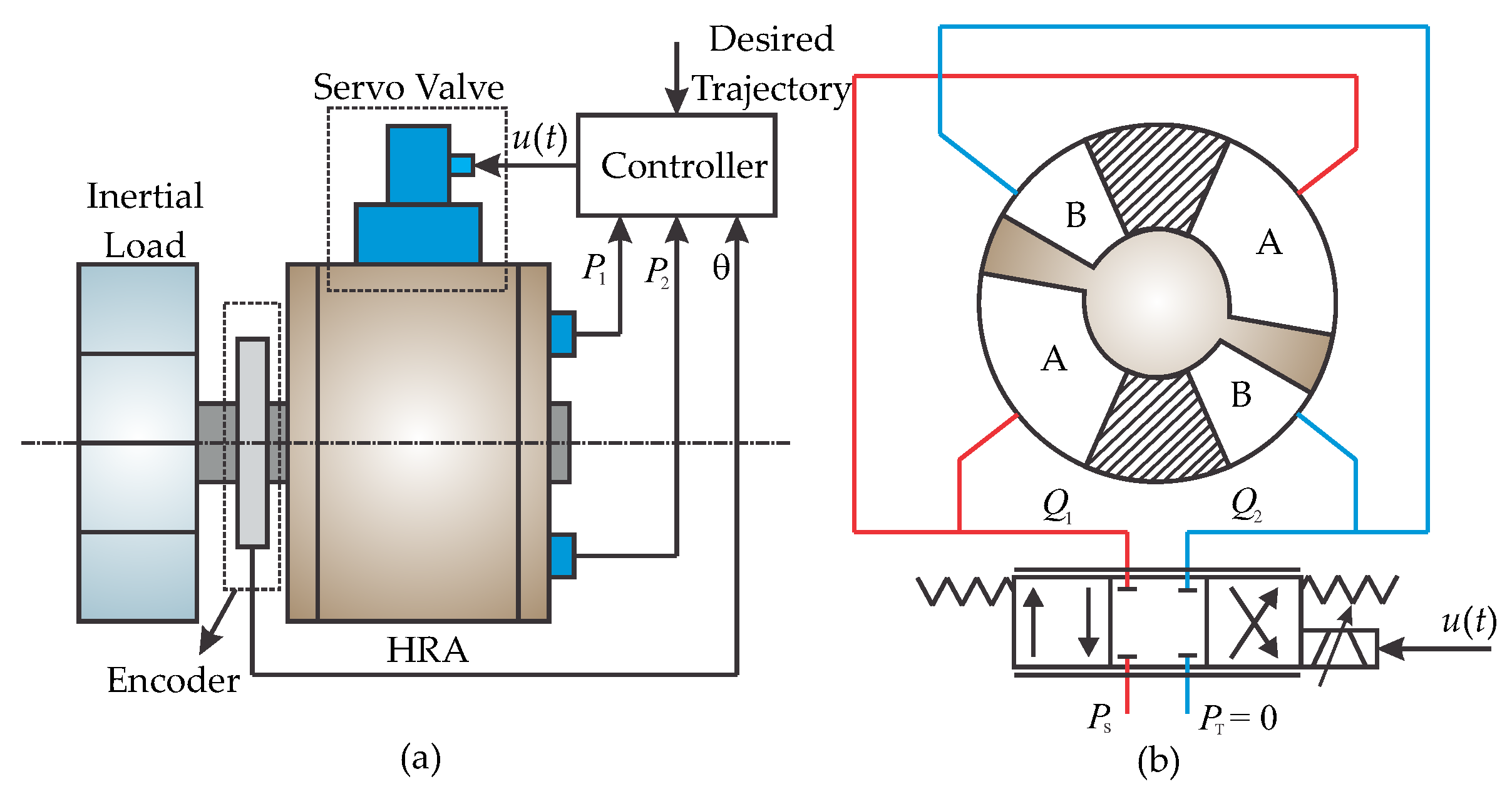
2. System Modeling and Problem Placement

The control system architecture of the considered EHS is illustrated in Figure 1. The angular position of the inertial load is exactly measured by a high-resolution encoder, whereas two pressure transducers are adopted to precisely observe the pressures in the two chambers of the HRA. The main control element of the system is a high-bandwidth servo valve used to manipulate the motion of the inertial load.

2.1. System Modeling

Applying the second Newton’s law, the motion dynamics of the inertial load can be derived by

$$J\ddot{\theta }=D_m{P}_L-B\dot{\theta }-A_f{S}_f\left(\dot{\theta }\right)-{\tau }_d$$

(1)

where J and $\theta$ denote the inertial moment and angular position of the load, respectively; $D_m$ and $P_L=P_1-P_2$ correspond to the radian displacement and pressure difference, i.e., load pressure, between two chambers with $P_1$ and $P_2$ signify the pressures in the forward and reverse chambers of the HRA, respectively; B reflexes the total viscous friction coefficient; $A_f$ represents the magnitude of Coulomb friction with known shape defined by the $S_f$ function [52]; and ${\tau }_d$ is the lumped uncertainty due to unknown external load, model uncertainties, and parametric deviations.

The load pressure dynamics are given by [53]

$$\frac{V_t}{4{\beta }_e}{\dot{P}}_L=-D_m\dot{\theta }+Q_L-C_t{P}_L+q\left(t\right)$$

(2)

where $V_t$ is the total control volume of the HRA, ${\beta }_e$ represents the effective buck modulus of the hydraulic fluid, $C_t$ denotes the internal leakage coefficient, $q\left(t\right)$ reflexes the grouped uncertain term caused by modeling errors and parameter deviations, and $Q_L$ is the load flow rate which is defined by [53]

$$Q_L=k_q{x}_v\sqrt{(P_S-\mathrm{sign}\left(x_v\right)P_L)}$$

(3)

where $k_q=C_{d}w\sqrt{1/\rho }$ is the flow gain, $C_d$ represents the discharge coefficient, w is the spool valve area gradient, and $\rho$ is the density of the hydraulic fluid. $x_v$ denotes the valve spool displacement which is proportional to the control signal u applied to the servo valve [44,52,54], i.e., $x_v=k_{u}u$, $k_u>0$ is the servo valve coefficient; $k_t=k_q{k}_u$ signifies the total flow gain with respect to u; $P_S$ is the supply pressure; and $\mathrm{sign}(•)$ is the standard signum function.

Set $\mathbf{x}={[x_1,x_2,x_3]}^T\stackrel{\Delta }{=}{[\theta ,\dot{\theta },D_m{P}_L/J]}^T$ as the system state vector. According to (1)–(3), the whole system dynamics can be obtained in the state-state representation as

$$\begin{array}{cc}\hfill & {\dot{x}}_1=x_2\hfill \\ \hfill & {\dot{x}}_2=x_3+f_2\left(\mathbf{x}\right)+d_1\left(t\right)\hfill \\ \hfill & {\dot{x}}_3=f_3\left(\mathbf{x}\right)+g_3(\mathbf{x},u)u+d_2\left(t\right)\hfill \end{array}$$

(4)

where $f_2\left(\mathbf{x}\right)$, $f_3\left(\mathbf{x}\right)$, $g_3(\mathbf{x},u)$, $d_1\left(t\right)$, and $d_2\left(t\right)$ are given by

$$\begin{array}{cc}\hfill & f_2\left(\mathbf{x}\right)=-\frac{B}{J}{x}_2-\frac{A_f}{J}{S}_f\left(x_2\right)\hfill \\ \hfill & f_3\left(\mathbf{x}\right)=-\frac{4D_m^2{\beta }_e}{J{V}_t}{x}_2-\frac{-4{\beta }_e{C}_t}{V_t}{x}_3\hfill \\ \hfill & g_3(\mathbf{x},u)=\frac{4D_m{\beta }_e{k}_t}{J{V}_t}\sqrt{\frac{1}{\rho }(P_S-\mathrm{sign}\left(u\right)\frac{J}{D_m}{x}_3)}\hfill \\ \hfill & d_1\left(t\right)={\tau }_d/J;d_2\left(t\right)=\frac{4D_m{\beta }_e}{J{V}_t}q\left(t\right)\hfill \end{array}$$

2.2. Problem Statement

The primary control objective is to design a control law that can achieve a prescribed tracking performances including overshoot, convergence rate, and steady-state tracking error under the effects of disturbances on the mechanical and hydraulic systems with both smooth and non-smooth desired reference trajectories and the nominal system parameters are assumed to be known.

To facilitate the control and observer design, the following reasonable assumptions are given as

Assumption A1

([6,7]). The pressures $P_1$, $P_2$ and the load pressure $P_L$ are bounded by the supply pressure $P_S$ to guarantee that the function $g_3(\mathbf{x},u)$ is strictly positive.

Assumption A2

([52]). The mismatched and matched lumped disturbances $d_1\left(t\right)$ and $d_2\left(t\right)$ are bounded, and their first-order derivatives are bounded by constants; i.e., $\left|{\dot{d}}_1\left(t\right)\right|\le {\delta }_1$ and $\left|{\dot{d}}_2\left(t\right)\right|\le {\delta }_2$.

Assumption A3

([44]). The function $f_2\left(\mathbf{x}\right)$ and $f_3\left(\mathbf{x}\right)$ are globally Lipschitz with respect to $x_2$; and $g_3\left(\mathbf{x}\right)$ is also Lipschitz in the working condition. Their Lipschitz constants are $k_{f_2}$, $k_{f_3}$, and $k_{g_3}$, respectively.

Lemma 1.

Consider the following Lyapunov function V satisfying

$$\dot{V}\le -a{V}^{\gamma }$$

(5)

where $a>0$ and $0<\gamma <1$. It can be recognized that, V converges to origin in finite time $t_f$ determined by

$$t_f\le \frac{V^{1-\gamma }\left(0\right)}{a(1-\gamma )}$$

(6)

Proof. 

The inequality (5) can be rewritten as

$$\begin{array}{cc}\hfill & V^{-\gamma }\dot{V}\le -a\iff \frac{1}{1-\gamma }\frac{d{V}^{1-\gamma }}{dt}\le -a\hfill \\ \hfill & \Rightarrow d{V}^{1-\gamma }\le -a(1-\gamma )dt\hfill \end{array}$$

(7)

Integrating both side of (7), the converging time is bounded by

$$t_f=\frac{V^{1-\gamma }\left(0\right)}{a(1-\gamma )}$$

(8)

This completes the proof of Lemma 1. □

Lemma 2

([6]). Considering a Lyapunov function V that satisfy the following inequality

$$\dot{V}\le -aV+b$$

(9)

where a and b are positive constants.

The function V reaches a region whose bound is determined by $b/a$ as $t\to \infty$, i.e., globally ultimately uniformly bounded stability (GUUB) is achieved.

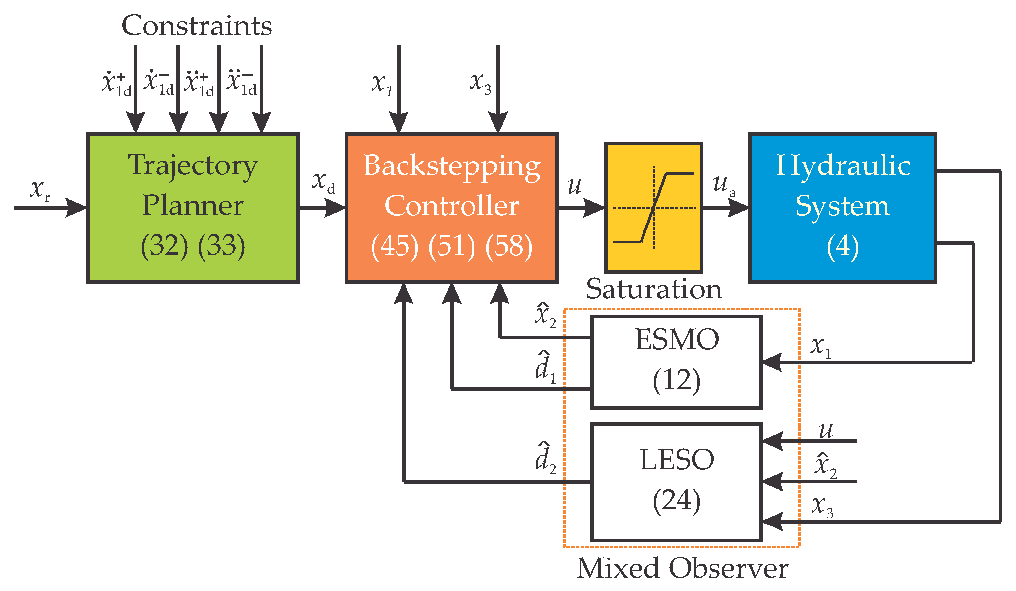
3. Active Disturbance Rejection Control Design

The proposed control strategy is illustrated in Figure 2. In order to actively compensate for the effects of both lumped mismatched and matched uncertainties and the lack of angular velocity measurement, the two observers, i.e., an ESMO and a LESO, are constructed. Consequently, the estimated velocity and generalized disturbances are fed back into the main controller whose input generated from a trajectory planner. Inherited from [19], a nonlinear variable structure filter-based trajectory planner with minor modifications is developed to relax the demand on smooth reference trajectory of the conventional backstepping technique by considering the kinematic constraints of the physical system. The designs of observers, trajectory planner, and main control strategy will be deliberately presented in the following sections.

3.1. Observer Design

3.1.1. Extended Sliding Mode Observer Design

Consider the mechanical system which is constituted by the first two equations of (4) as

$$\begin{array}{cc}\hfill & {\dot{x}}_1=x_2\hfill \\ \hfill & {\dot{x}}_2=x_3+f_2\left(\mathbf{x}\right)+d_1\left(t\right)\hfill \end{array}$$

(10)

By extending $x_{e1}=d_1\left(t\right)$ as a new state and $h_1\left(t\right)$ as the derivative of $x_{e1}$, the system dynamics (10) can be rewritten as

$$\begin{array}{cc}\hfill & {\dot{x}}_1=x_2\hfill \\ \hfill & {\dot{x}}_2=x_3+f_2\left(\mathbf{x}\right)+x_{e1}\hfill \\ \hfill & {\dot{x}}_{e1}=h_1\left(t\right)\hfill \end{array}$$

(11)

To estimate the angular velocity $x_2$ of the actuator and lumped disturbance $d_1\left(t\right)$, the ESMO is constructed as

$$\begin{array}{cc}\hfill & {\dot{\widehat{x}}}_1={\widehat{x}}_2+{\ell }_1\mathrm{sign}(x_1-{\widehat{x}}_1)\hfill \\ \hfill & {\dot{\widehat{x}}}_2=x_3+f_2\left(\widehat{\mathbf{x}}\right)+{\widehat{x}}_{e1}+2{\omega }_1{\ell }_1\mathrm{sign}(x_1-{\widehat{x}}_1)\hfill \\ \hfill & {\dot{\widehat{x}}}_{e1}={\omega }_1^2{\ell }_1\mathrm{sign}(x_1-{\widehat{x}}_1)\hfill \end{array}$$

(12)

where ${\ell }_1$ is a positive constant and ${\omega }_1$ is the observer bandwidth determined later.

Let ${\tilde{x}}_i=x_i-{\widehat{x}}_i$ being the estimation error with $i=1,2,e1$. From (11) and (12), error dynamics of the observer are determined by

$$\begin{array}{cc}\hfill & {\dot{\tilde{x}}}_1={\tilde{x}}_2-{\ell }_1\mathrm{sign}\left({\tilde{x}}_1\right)\hfill \\ \hfill & {\dot{\tilde{x}}}_2={\tilde{f}}_2+{\tilde{x}}_{e1}-2{\omega }_1{\ell }_1\mathrm{sign}\left({\tilde{x}}_1\right)\hfill \\ \hfill & {\dot{\tilde{x}}}_{e1}=h_1\left(t\right)-{\omega }_1^2{\ell }_1\mathrm{sign}\left({\tilde{x}}_1\right)\hfill \end{array}$$

(13)

Theorem 1.

By employing the ESMO (12), Bthe angular velocity of the HRA and lumped mismatched disturbance estimation errors, i.e., ${\tilde{x}}_2$ and ${\tilde{x}}_{e1}$, approach to arbitrarily small bounded regions whose boundaries depend on the selection of observer bandwidth ${\omega }_1$.

Proof of Theorem 1.

Consider a Lyapunov function as

$$V_{x_1}=\frac{1}{2}{\tilde{x}}_1^2$$

(14)

Taking time derivative of it and combining with (13) yields

$$\begin{array}{cc}\hfill {\dot{V}}_{x_1}& ={\tilde{x}}_1{\dot{\tilde{x}}}_1\hfill \\ \hfill & ={\tilde{x}}_1({\tilde{x}}_2-{\ell }_1\mathrm{sign}\left({\tilde{x}}_1\right))\hfill \\ \hfill & \le -({\ell }_1-|{\tilde{x}}_2\left|\right)|{\tilde{x}}_1|\hfill \end{array}$$

(15)

Obviously, in the region $|{\tilde{x}}_2|\le {\ell }_1-{\ell }_0$ with ${\ell }_0>0$, the following inequality holds

$${\dot{V}}_{x_1}\le -{\ell }_0\left|{\tilde{x}}_1\right|$$

(16)

When sliding mode occurs, the reduced-order system dynamics are equivalent to ${\tilde{x}}_2=k_1\mathrm{sign}\left({\tilde{x}}_1\right)$, hence, (13) becomes

$$\begin{array}{cc}\hfill & {\dot{\tilde{x}}}_2={\tilde{f}}_2+{\tilde{x}}_{e1}-2{\omega }_1{\tilde{x}}_2\hfill \\ \hfill & {\dot{\tilde{x}}}_{e1}=h_1\left(t\right)-{\omega }_1^2{\tilde{x}}_2\hfill \end{array}$$

(17)

Define the scale estimation error vector as $\epsilon ={[{\epsilon }_1,{\epsilon }_2]}^T={[{\tilde{x}}_2,{\tilde{x}}_{e1}/{\omega }_1]}^T$, (17) is rewritten as

$$\dot{\epsilon }={\omega }_1{A}_1\epsilon +B_1{\tilde{f}}_2+C_1\frac{h_1\left(t\right)}{{\omega }_1}$$

(18)

where

$$A_1=\left[\begin{array}{cc}-2& 1\\ -1& 0\end{array}\right];B_1=\left[\begin{array}{c}1\\ 0\end{array}\right];C_1=\left[\begin{array}{c}0\\ 1\end{array}\right]$$

Because the matrix $A_1$ is Hurwitz, there exists a symmetric positive definite matrix $P_1$ that satisfies the following Lyapunov equation

$$A_1^T{P}_1+P_1{A}_1=-2I_2$$

(19)

where $I_2$ is the identity matrix of size 2.

Consider the following Lyapunov function

$$V_{\epsilon }=\frac{1}{2}{\epsilon }^T{P}_1\epsilon$$

(20)

Taking time derivative of (20), one obtains

$${\dot{V}}_{\epsilon }=-{\omega }_1{\epsilon }^T\epsilon +{\epsilon }^T{P}_1{B}_1{\tilde{f}}_2+{\epsilon }^T{P}_1{C}_1\frac{h_1\left(t\right)}{{\omega }_1}$$

(21)

Applying Young’s inequalities, we have

$$\begin{array}{cc}\hfill {\dot{V}}_{\epsilon }& \le -({\omega }_1-\frac{1}{2}{\lambda }_{\max }\left(X_1\right)k_{f_2}^2-1){\epsilon }^T\epsilon +\frac{1}{2{\omega }_1^2}{\lambda }_{\max }\left(Y_1\right){\delta }_1^2\hfill \\ \hfill & \le -a_1{V}_{\epsilon }+b_1\hfill \end{array}$$

(22)

where $X_1=B_1^T{P}_1^T{P}_1{B}_1$, $Y_1=C_1^T{P}_1^T{P}_1{C}_1$; ${\lambda }_{\max }\left(X_1\right)$, and ${\lambda }_{\max }\left(Y_1\right)$ are the maximum eigenvalues of the matrices $X_1$ and $Y_1$, respectively.

$$\begin{array}{cc}\hfill & a_1=\frac{1}{{\lambda }_{\max }\left(P1\right)}({\omega }_1-\frac{1}{2}{\lambda }_{\max }\left(X_1\right)k_{f_2}^2-1)\hfill \\ \hfill & b_1=\frac{1}{2{\omega }_1^2}{\lambda }_{\max }\left(Y_1\right){\delta }_1^2\hfill \end{array}$$

(23)

where ${\lambda }_{\max }\left(P_1\right)$ is the maximal eigenvalue of the matrix $P_1$.

Theorem 1 is completely proven. □

Remark 1.

To eliminate the chattering in the estimated values of the mismatched disturbance and angular velocity, the “$\mathrm{sign}$” function in (12) is replaced by the hyperbolic tangent function, i.e., “$\tanh$” function.

3.1.2. Matched Disturbance Observer Design

Since the load pressure $P_L$ can be directly calculated through measured pressures $P_1$ and $P_2$ in the forward chamber and reverse chamber of the HRA, respectively, the LESO is constructed to estimate the lumped disturbance in the hydraulic system as

$$\begin{array}{cc}\hfill & {\dot{\widehat{x}}}_3=f_3\left(\widehat{\mathbf{x}}\right)+g_3(\widehat{\mathbf{x}},u)u+{\widehat{x}}_{e2}+2{\omega }_2(x_3-{\widehat{x}}_3)\hfill \\ \hfill & {\dot{\widehat{x}}}_{e2}={\omega }_2^2(x_3-{\widehat{x}}_3)\hfill \end{array}$$

(24)

where $x_{e2}=d_2\left(t\right)$ and ${\dot{x}}_{e2}=h_2\left(t\right)$ with $h_2\left(t\right)$ is the first-order derivative of $d_2\left(t\right)$.

Set ${\tilde{x}}_3=x_3-{\widehat{x}}_3$ and ${\tilde{x}}_{e2}=x_{e2}-{\widehat{x}}_{e2}$ as the estimation errors, the estimator error dynamics of the LESO are given by

$$\begin{array}{cc}\hfill & {\dot{\tilde{x}}}_3={\tilde{f}}_3+{\tilde{x}}_{e2}-2{\omega }_2{\tilde{x}}_3\hfill \\ \hfill & {\dot{\tilde{x}}}_{e2}=h_2\left(t\right)-{\omega }_2^2{\tilde{x}}_3\hfill \end{array}$$

(25)

where ${\tilde{f}}_3=f_3\left(\mathbf{x}\right)-f_3\left(\widehat{\mathbf{x}}\right)$, and ${\omega }_2$ is the bandwidth of the constructed LESO.

Defining $\eta ={[{\eta }_1,{\eta }_2]}^T={[{\tilde{x}}_3,{\tilde{x}}_{e2}/{\omega }_2]}^T$ as scaled estimation error vector, the error dynamics (25) can be transformed into

$$\dot{\eta }={\omega }_2{A}_2\eta +B_2{\tilde{f}}_3+C_2\frac{h_2\left(t\right)}{{\omega }_2}$$

(26)

where

$$A_2=\left[\begin{array}{cc}-2& 1\\ -1& 0\end{array}\right];B_2=\left[\begin{array}{c}1\\ 0\end{array}\right];C_2=\left[\begin{array}{c}0\\ 1\end{array}\right]$$

Since the matrix $A_2$ is strictly negative definite, there exists a symmetric positive definite $P_2$ that satisfies the following Lyapunov equality

$$A_2^T{P}_2+P_2{A}_2=-2I_2$$

(27)

where $I_2$ is the identity matrix of size 2.

Theorem 2.

The established LESO guarantees that the estimation error of the lumped matched disturbance $d_2\left(t\right)$ converge to an arbitrarily small bounded region whose boundary depends on the selection of the observer gain ${\omega }_2$ and the estimation accuracy of $x_2$ of the above ESMO.

Proof of Theorem 2.

Consider the following candidate Lyapunov function

$$V_{\eta }=\frac{1}{2}{\eta }^T{P}_2\eta$$

(28)

Differentiating (28) with respect to time yields

$${\dot{V}}_{\eta }=-{\omega }_2{\eta }^T\eta +{\eta }^T{P}_2{B}_2{\tilde{f}}_3+{\eta }^T{P}_2{C}_2\frac{h_2\left(t\right)}{{\omega }_2}$$

(29)

Applying Young’s inequality, we have

$$\begin{array}{cc}\hfill {\dot{V}}_{\eta }& \le -{\omega }_2{\eta }^T\eta +\frac{1}{2}{\eta }^T\eta +\frac{1}{2}{B}_2^T{P}_2^T{P}_2{B}_2{\tilde{f}}_3^2+\frac{1}{2}{\eta }^T\eta +\frac{1}{2}{C}_2^T{P}_2^T{P}_2{C}_2\frac{h_2^2\left(t\right)}{{\omega }_2^2}\hfill \\ \hfill & \le -({\omega }_2-1){\eta }^T\eta +\frac{1}{2}{\lambda }_{\max }\left(X_2\right)k_{f_3}{\tilde{x}}_2^2+\frac{1}{2}{\lambda }_{\max }\left(Y_2\right)\frac{{\delta }_2^2}{{\omega }_2^2}\hfill \end{array}$$

(30)

As stated in Theorem 1, it can be observed that ${\tilde{x}}_2$ converges to the arbitrarily small region, hence, a globally ultimately bounded stability of the LESO is ensured. The bound of this region is specified by the designed observer bandwidths ${\omega }_1$ and ${\omega }_2$.

This completes the proof of Theorem 2. □

Remark 2.

By appropriately choosing the switching gain ${\ell }_1$ and the bandwidth ${\omega }_1$ of the ESMO, the estimation errors of immeasurable velocity and lumped mismatched uncertainty reach arbitrarily small bounded regions. The estimation accuracy of the generalized matched disturbance in hydraulic dynamics depends on not only the bandwidth of the LESO, i.e., ${\omega }_2$ but also the estimation accuracy of the angular velocity.

3.2. Trajectory Planner Design

It is worth noting that for the conventional backstepping, the desired reference trajectory should be carefully designed to be sufficiently smooth and bounded, and its derivatives are also continuous and bounded. Therefore, it is extremely challenging to maintain a high-accuracy tracking performance of the closed-loop system in the case of step reference trajectories. Inherited from [19], a modified nonlinear filter-based trajectory planner for online trajectory planning is utilized to transform the original trajectory into an appropriate one by considering the system constraints, whose structure is depicted in Figure 3.

Therefore, the trajectory planner guarantees its output, i.e., newly reference trajectory, is smooth, tracks the original reference trajectory in minimum time without overshoot, and satisfies the prescribed kinematic constraints, i.e., lower bound and upper bound of velocity and acceleration, depending on the system specifications. The mathematical representation of this planner is as follows:

The integrator chains are mathematically represented as

$$\left[\begin{array}{c}{x}_{1d}(k+1)\\ {\dot{x}}_{1d}(k+1)\end{array}\right]=\left[\begin{array}{cc}1& T\\ 0& 1\end{array}\right]\left[\begin{array}{c}{x}_{1d}\left(k\right)\\ {\dot{x}}_{1d}\left(k\right)\end{array}\right]+\left[\begin{array}{c}{T}^2/\phantom{T^{2}2}2\\ T\end{array}\right]u\left(k\right)$$

(31)

where the pair $(x_{1d}\left(k\right),{\dot{x}}_{1d}\left(k\right))$ represents the state vector, T is the system sampling time, $u\left(k\right)={\ddot{x}}_{1d}\left(k\right)$ is the control action of the integrator chain, and k denotes the sample number, i.e., $t\left(k\right)=kT$.

Compared to [19], the control law $u\left(k\right)$ is redesigned as

$$u\left(k\right)=\left\{\begin{array}{cc}\hfill {\ddot{x}}_{1d}^{-}\tanh \left(C_{tp}\sigma \left(k\right)\right),& \mathrm{if}\sigma \left(k\right)\ge 0\hfill \\ \hfill -{\ddot{x}}_{1d}^{+}\tanh \left(C_{tp}\sigma \left(k\right)\right),& \mathrm{otherwise}\hfill \end{array}\right.$$

(32)

where $C_{tp}$ is a positive constant, $\sigma \left(k\right)=\dot{z}\left(k\right)-\dot{\tilde{z}}\left(k\right)$ with $\dot{z}\left(k\right)$ and $\dot{\tilde{z}}\left(k\right)$ are determined via following equations

$$\begin{array}{cc}\hfill & {\dot{z}}^{+}=-\frac{{\dot{x}}_{1d}^{+}-{\dot{x}}_r\left(k\right)}{T{\ddot{x}}_{1d}^{-}};z^{+}=⌈{\dot{z}}^{+}⌉\left[{\dot{z}}^{+}-\frac{⌈{\dot{z}}^{+}⌉-1}{2}\right]\hfill \\ \hfill & {\dot{z}}^{-}=-\frac{{\dot{x}}_{1d}^{-}-{\dot{x}}_r\left(k\right)}{T{\ddot{x}}_{1d}^{+}};z^{+}=⌈-{\dot{z}}^{-}⌉\left[-{\dot{z}}^{-}-\frac{⌈-{\dot{z}}^{-}⌉-1}{2}\right]\hfill \\ \hfill & \left[\alpha ,\beta \right]=\left\{\begin{array}{cc}\hfill \left[{\ddot{x}}_{1d}^{+},{\ddot{x}}_{1d}^{-}\right],& \mathrm{if}\frac{y\left(k\right)}{T}+\frac{\dot{y}\left(k\right)}{2}>0\hfill \\ \hfill \left[{\ddot{x}}_{1d}^{-},{\ddot{x}}_{1d}^{+}\right],& \mathrm{otherwise}\hfill \end{array}\right.\hfill \\ \hfill & z\left(k\right)=\frac{1}{T\alpha }\left|\frac{y\left(k\right)}{T}+\frac{\dot{y}\left(k\right)}{2}\right|\hfill \\ \hfill & \gamma \left(k\right)=\left\{\begin{array}{cc}\hfill z^{+},& \mathrm{if}z\left(k\right)<z^{+}\hfill \\ \hfill z\left(k\right),& \mathrm{if}{z}^{+}\le z\left(k\right)\le z^{-}\hfill \\ \hfill z^{-},& \mathrm{if}z\left(k\right)>z^{-}\hfill \end{array}\right.\hfill \\ \hfill & m\left(k\right)=⌊\frac{1+\sqrt{1+8\left|\gamma \right(k\left)\right|}}{2}⌋\hfill \\ \hfill & \dot{\tilde{z}}\left(k\right)=-\frac{\gamma \left(k\right)}{m\left(k\right)}-\frac{m\left(k\right)-1}{2}\mathrm{sign}\left(\gamma \left(k\right)\right)\hfill \\ \hfill & \dot{z}\left(k\right)=\left\{\begin{array}{c}\frac{\dot{y}\left(k\right)}{T\left|\alpha \right|},\mathrm{if}\left[\left(z\left(k\right)\ge 0\&\frac{\dot{y}\left(k\right)}{T\left|\alpha \right|}\le \dot{\tilde{z}}\left(k\right)\right)\mathrm{or}\left(z_k<0\&\frac{\dot{y}\left(k\right)}{T\left|\alpha \right|}\right)\right]\hfill \\ \frac{\dot{y}\left(k\right)}{T\left|\beta \right|}+\left(\frac{m\left(k\right)-1}{2}+\frac{\left|\gamma \right(k\left)\right|}{m\left(k\right)}\right)\frac{\alpha +\beta }{\left|\beta \right|},\mathrm{otherwise}\hfill \end{array}\right.\hfill \end{array}$$

(33)

where ${\ddot{x}}_{1d}^{-}$, ${\dot{x}}_{1d}^{-}$; ${\ddot{x}}_{1d}^{+}$, and ${\dot{x}}_{1d}^{+}$ are the lower bounds and upper bounds of the acceleration and velocity so-called kinematic constraints of the system, i.e., ${\dot{x}}_{1d}^{-}\le {\dot{x}}_{1d}\le {\dot{x}}_{1d}^{+}$ and ${\ddot{x}}_{1d}^{-}\le {\ddot{x}}_{1d}\le {\ddot{x}}_{1d}^{+}$, respectively; ${\dot{x}}_r$ and ${\dot{x}}_r$ denote the original desired velocity and acceleration, respectively; $y\left(k\right)=x_{1d}\left(k\right)-x_r\left(k\right)$ represents the filter tracking error, and $\dot{y}\left(k\right)={\dot{x}}_{1d}\left(k\right)-{\dot{x}}_r\left(k\right)$ reflexes the filter velocity error; $⌊•⌋$ and $⌈•⌉$ correspond to the floor and ceil functions of their arguments.

For the sake of conciseness, the theoretical proof of the trajectory planner is omitted in this paper. Refer to [19] for details.

Remark 3.

The primary purpose of construction of the trajectory planner is to relax the restriction on the requirement of sufficient smooth reference trajectories of the conventional backstepping framework. In addition, by considering the kinematic constraints of the EHS, the stress on the actual control input is significantly mitigated. Besides, since the filtered trajectory always commences from zero, the initial matching condition is satisfied to avoid the saturation of the control input effectively as a result.

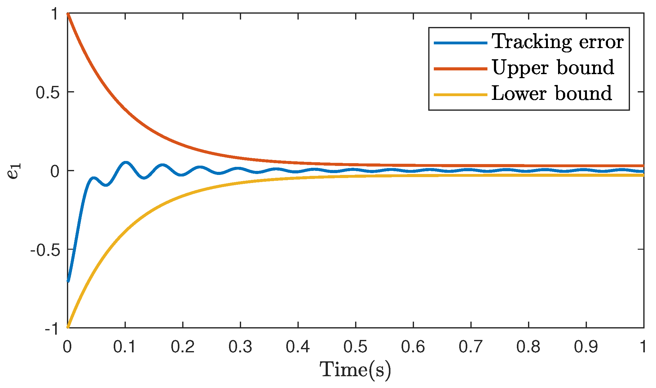
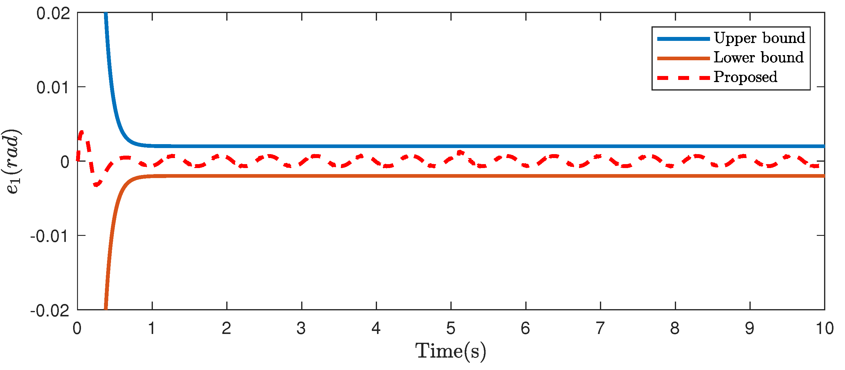
3.3. Controller Design with Prescribed Tracking Performance

The primary control objective is to design a control law that ensures the output tracking error, i.e., ${ϵ}_1=x_1-x_{1d}$, satisfies the prescribed tracking performances including convergence rate, overshoot, and steady-state error under both smooth and abruptly changing reference trajectories.

The desired performance function is defined by

$$\rho \left(t\right)=({\rho }_0-{\rho }_{\infty })e^{-\varphi t}+{\rho }_{\infty }$$

(34)

where $\varphi >0$ signifies the convergence rate, ${\rho }_0>0$ and ${\rho }_{\infty }>0$ are determined as

$$\underset{t\to 0}{lim}\rho \left(t\right)={\rho }_0;\underset{t\to \infty }{lim}\rho \left(t\right)={\rho }_{\infty };\mathrm{and}{\rho }_0>{\rho }_{\infty }$$

(35)

Remark 4.

The function (34) is strictly positive monotonically decreasing and bounded. This function converges to a small value defined by ${\rho }_{\infty }$ which can be regarded to be the steady-state error, whereas ${\rho }_0$ can be thought as the initial error and ϕ designates the convergence rate of the error.

The design control algorithm must guarantee that the output tracking error $e_1$ satisfies the inequality, i.e., prescribed tracking performance, presented as follows:

$$-\underline{\upsilon }\rho \left(t\right)<e_1<\overline{\upsilon }\rho \left(t\right),\forall t\ge 0$$

(36)

where $\underline{\upsilon }$ and $\overline{\upsilon }$ are the positive constants selected by designers. To do so, the initial tracking error must satisfy $e_1\left(0\right)>-\underline{\upsilon }\rho \left(0\right)$ and $e_1\left(0\right)<\overline{\upsilon }\rho \left(0\right)$. The figurative illustration of the prescribed tracking performance control is depicted in Figure 4.

The above condition can be transformed into

$${ϵ}_1=\rho \left(t\right)S\left(z_1\right)$$

(37)

where $S\left(z_1\right)$ is a smooth and monotonically increasing function that is mathematically represented as

$$S\left(z_1\right)=\frac{\overline{\upsilon }{e}^{z_1}-\underline{\upsilon }{e}^{-z_1}}{e^{z_1}+e^{-z_1}}$$

(38)

From the definition of the function $S\left(z_1\right)$, some interesting features of it can be listed as follows:

(1)

$-\underline{\upsilon }<S\left(z_1\right)<\overline{\upsilon }$

(2)

$\underset{z_1\to +\infty }{lim}S\left(z_1\right)=\overline{\upsilon }$ and $\underset{z_1\to -\infty }{lim}S\left(z_1\right)=\underline{\upsilon }$

From (37) and (38), the conversion error $z_1$ of the actual tracking error $e_1$ can be expressed by

$$z_1=\frac{1}{2}log\frac{\lambda +\underline{\upsilon }}{\overline{\upsilon }-\lambda }$$

(39)

where $\lambda ={ϵ}_1/\rho \left(t\right)$ and $\log (•)$ is the natural logarithm operator of •.

Remark 5.

The prescribed tracking performance (36) is equivalent to the bounded tracking of the conversion error $z_1$. It means that when $z_1$ is bounded, the prescribed performance (36) is always satisfied.

Taking time derivative of (39) yields

$${\dot{z}}_1=\frac{1}{2}\left(\frac{1}{\lambda +\underline{\upsilon }}+\frac{1}{\overline{\upsilon }-\lambda }\right)\left(\frac{{\dot{e}}_1}{\rho }-\frac{e_1\dot{\rho }}{{\rho }^2}\right)$$

(40)

Considering the system dynamics (4), one obtains

$${\dot{z}}_1=\zeta \left(x_2-{\dot{x}}_{1d}-\frac{e_1\dot{\rho }}{\rho }\right)$$

(41)

where $\zeta =\frac{1}{2\rho }\left(\frac{1}{\overline{\upsilon }-\lambda }+\frac{1}{\lambda +\underline{\upsilon }}\right)$.

To applying CF approach, the tracking error and compensated tracking error signal for the first step are designed as

$$\begin{array}{cc}\hfill & e_1=z_1\hfill \\ \hfill & v_1=e_1-{\xi }_1\hfill \end{array}$$

(42)

where the dynamic of ${\xi }_1$ is given by

$${\dot{\xi }}_1=-k_1{\xi }_1+\zeta \left(x_{2c}-{\alpha }_1\right)+\zeta {\xi }_2$$

(43)

with ${\xi }_1\left(0\right)=0$ and $x_{2c}$ is the filtered signal of ${\alpha }_1$ determined by

$$T_f{\dot{x}}_{2c}+x_{2c}={\alpha }_1$$

where the filter initial conditions are $x_{2c}\left(0\right)={\alpha }_1\left(0\right)$ and ${\dot{x}}_{2c}\left(0\right)=0$, and $T_f$ is time constant designed later.

A Lyapunov function is chosen as $V_1=1/2v_1^2$, taking time derivative of it then combining with (42) and, (43) we have

$$\begin{array}{cc}\hfill {\dot{V}}_1& =v_1{\dot{v}}_1\hfill \\ \hfill & =\zeta z_1\left(\zeta x_2-\zeta {\dot{x}}_{1d}-\zeta \frac{{\epsilon }_1\dot{\rho }}{\rho }+k_1{\xi }_1-\zeta x_{2c}+\zeta {\alpha }_1-\zeta {\xi }_2\right)\hfill \end{array}$$

(44)

Define $e_2=x_2-x_{2c}$ and $v_2=e_2-{\xi }_2$ as an auxiliary tracking error and compensated tracking error for the second step, respectively. The virtual control law ${\alpha }_1$ is chosen as

$${\alpha }_1={\dot{x}}_{1d}+\frac{{ϵ}_1\dot{\rho }}{\rho }-\frac{1}{\zeta }{k}_1{e}_1$$

(45)

Substituting (45) into (44) leads to

$${\dot{V}}_1=-k_1{v}_1^2+\zeta v_1{v}_2$$

(46)

The dynamic of ${\xi }_2$ is designed as

$${\dot{\xi }}_2=-k_2{\xi }_2+(x_{3c}-{\alpha }_2)+{\xi }_3$$

(47)

with ${\xi }_2\left(0\right)=0$ and $x_{3c}$ is the filtered signal of ${\alpha }_2$ determined by

$$T_f{\dot{x}}_{3c}+x_{3c}={\alpha }_2$$

where the filter initial conditions are $x_{3c}\left(0\right)={\alpha }_2\left(0\right)$ and ${\dot{x}}_{3c}\left(0\right)=0$.

A candidate Lyapunov function is chosen as

$$V_2=V_1+\frac{1}{2}{v}_2^2$$

(48)

Taking derivative of $V_2$ then combining with (4), (46) and (47), one obtains

$$\begin{array}{cc}\hfill {\dot{V}}_2& ={\dot{V}}_1+v_2{\dot{v}}_2\hfill \\ \hfill & =-k_1{v}_1^2+\zeta v_1{v}_2+v_2\left(f_2+\left(x_3-x_{3c}-{\xi }_3\right)+d_1-{\dot{x}}_{2c}+k_2{\xi }_2+{\alpha }_2\right)\hfill \end{array}$$

(49)

Hence, the virtual control ${\alpha }_2$ is designed as follows:

$${\alpha }_2=-f_2-d_1+{\dot{x}}_{2c}-\zeta v_1-k_2{e}_2$$

(50)

Since the terms $x_2$ and $d_1$ are immeasurable, their estimated value will be used, the virtual control ${\alpha }_2$ is reconstructed as

$${\alpha }_2=-{\widehat{f}}_2-{\widehat{x}}_{e1}+{\dot{x}}_{2c}-\zeta v_1-k_2({\widehat{x}}_2-x_{2c})$$

(51)

The derivative of $V_2$ is rewritten as

$$\begin{array}{cc}\hfill {\dot{V}}_2& =-k_1{v}_1^2+\zeta v_1{v}_2+v_2\left(f_2+v_3+d_1-{\dot{x}}_{2c}+k_2{\xi }_2+{\alpha }_2\right)\hfill \\ \hfill & =-k_1{v}_1^2-k_2{v}_2^2+v_2{v}_3+v_2{\tilde{f}}_2+v_2{\tilde{x}}_{e1}+k_2{v}_2{\tilde{x}}_2\hfill \end{array}$$

(52)

The tracking error of $x_3$ is given by

$$e_3=x_3-x_{3c}$$

(53)

The compensated tracking error is determined as

$$v_3=e_3-{\xi }_3$$

(54)

where the dynamic of ${\xi }_3$ is determined as

$${\dot{\xi }}_3=-k_3{\xi }_3$$

(55)

Define the Lyapunov function as

$$V_3=V_2+\frac{1}{2}{v}_3^2$$

(56)

Taking derivative of $V_3$, we have

$$\begin{array}{cc}\hfill {\dot{V}}_3& ={\dot{V}}_2+v_3{\dot{v}}_3\hfill \\ \hfill & =-k_1{v}_1^2-k_2{v}_2^2+v_2{v}_3+v_3\left(f_3+g_{3}u+d_2-{\dot{x}}_{3c}-{\dot{\xi }}_3\right)\hfill \end{array}$$

(57)

The actual control voltage applied to the system is designed as

$$u=\frac{1}{g_3}\left(-{\widehat{f}}_3-{\widehat{d}}_2+{\dot{x}}_{3c}-\left({\widehat{x}}_2-x_{2c}-{\xi }_2\right)-k_3{e}_3\right)$$

(58)

Substituting (58) and (55) into (57) yields

$$\begin{array}{c}\hfill {\dot{V}}_3=-k_1{v}_1^2-k_2{v}_2^2-k_3{v}_3^2+v_2{\tilde{f}}_2+v_2{\tilde{x}}_{e1}+k_2{v}_2{\tilde{x}}_2+v_3{\tilde{f}}_3+v_3{\tilde{x}}_{e2}-v_3{\tilde{x}}_2\end{array}$$

(59)

Theorem 3.

By employing control laws (45), (51), and (58) with regard to the CF approach with error compensation mechanisms (43), (47), (55), and ESMO (12), ESO (24), the closed-loop system output tracking capability satisfies the prescribed tracking performance defined in (36).

Proof of Theorem 3.

See Appendix A. □

4. Numerical Simulation and Discussion

4.1. Simulation Setup

The nominal system parameters of the studied EHS provided in

Table 1. Nominal system parameters of the studied EHS.

Parameter	Unit	Value	Parameter	Unit	Value
J	$\mathrm{kg}·{\mathrm{m}}^2$	0.2	$C_t$	${\mathrm{m}}^3·{\mathrm{s}}^{-1}·\mathrm{P}{\mathrm{a}}^{-1}$	$1\times {10}^{-12}$
B	$\mathrm{N}·\mathrm{m}·\mathrm{s}·\mathrm{ra}{\mathrm{d}}^{-1}$	90	$P_s$	$\mathrm{Pa}$	$1\times {10}^7$
$D_m$	${\mathrm{m}}^3·{\mathrm{rad}}^{-1}$	$5.8\times {10}^{-5}$	$A_f$	$\mathrm{N}·\mathrm{m}$	10
${\beta }_e$	$\mathrm{Pa}$ or $\mathrm{N}·{\mathrm{m}}^{-2}$	$7\times {10}^8$	$V_t$	${\mathrm{m}}^3$	$1.16\times {10}^{-4}$
$k_t$	${\mathrm{m}}^3·{\mathrm{s}}^{-1}·{\mathrm{V}}^{-1}·\mathrm{P}{\mathrm{a}}^{-1/\phantom{12}2}$	$1.1969\times {10}^{-8}$

are used to design the main control strategy and observers.

To demonstrate the effectiveness of the proposed control strategy, the following controllers are employed for comparison as:

(1)

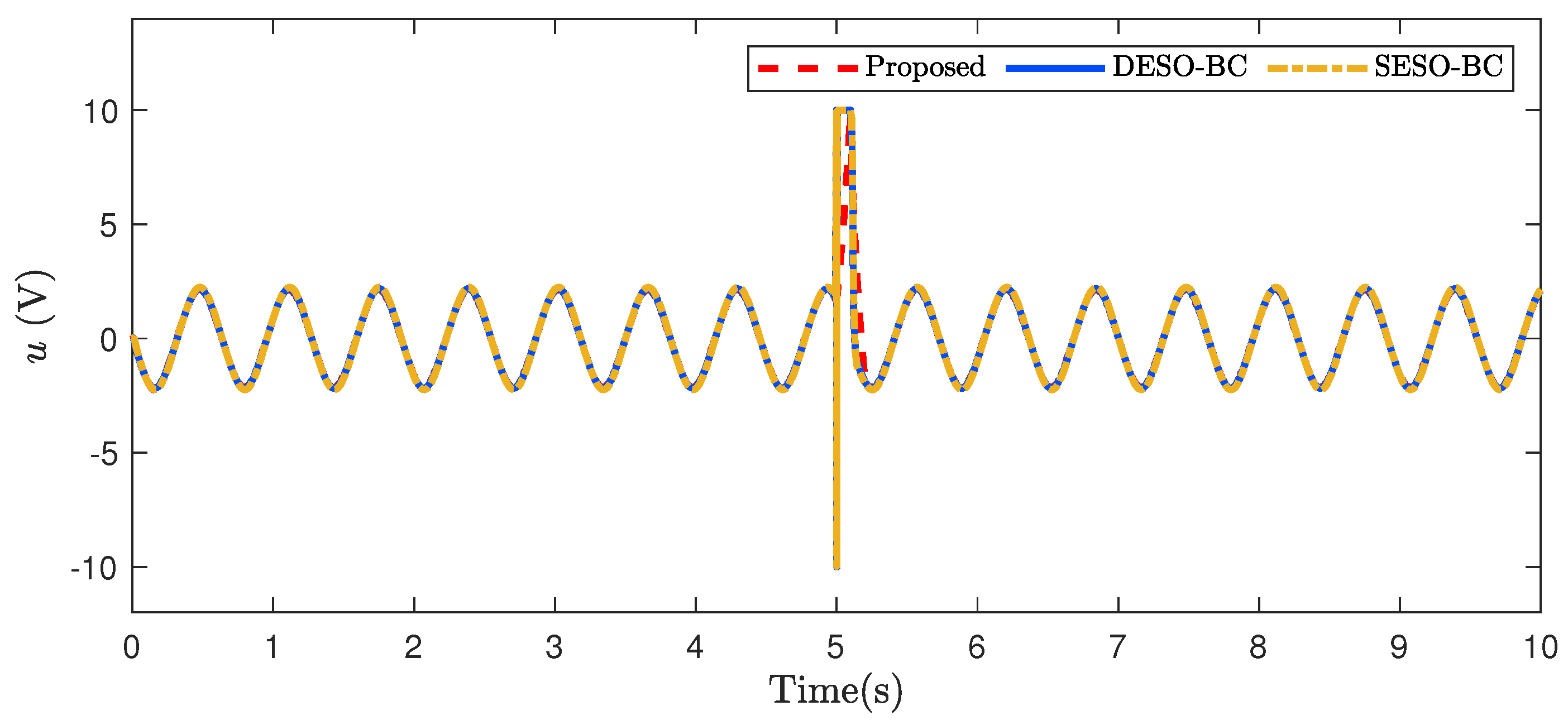
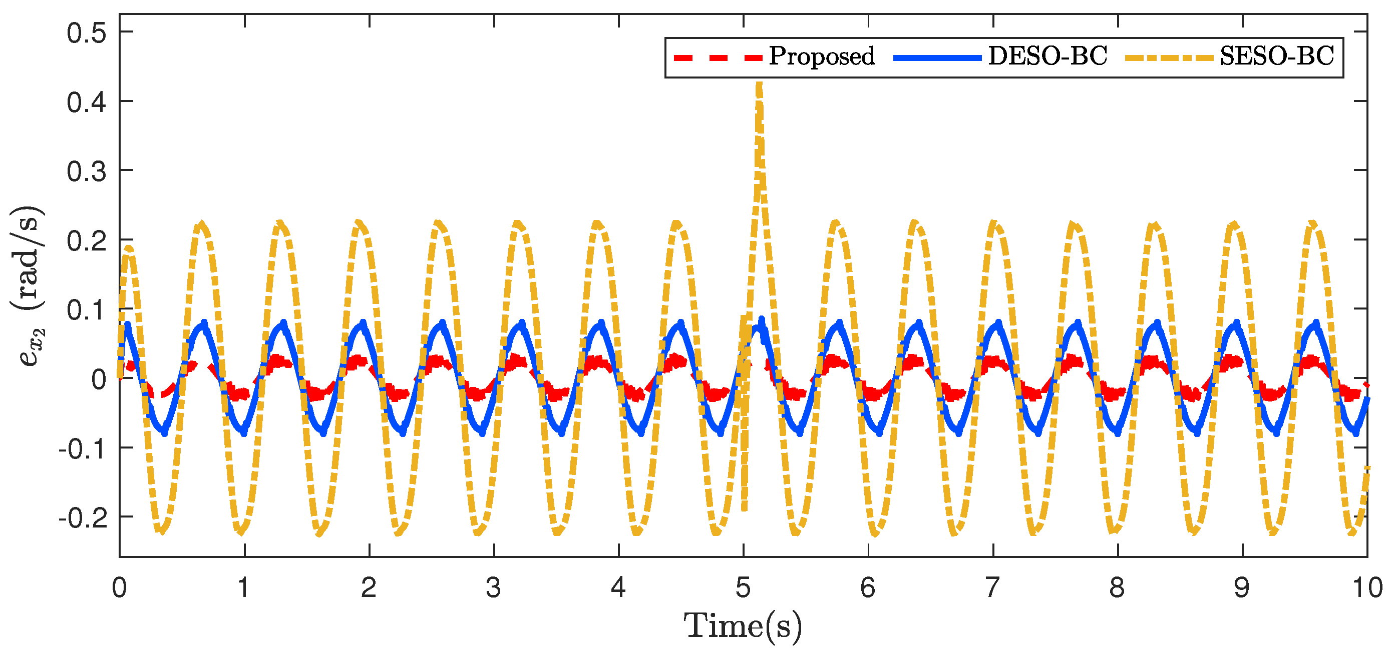
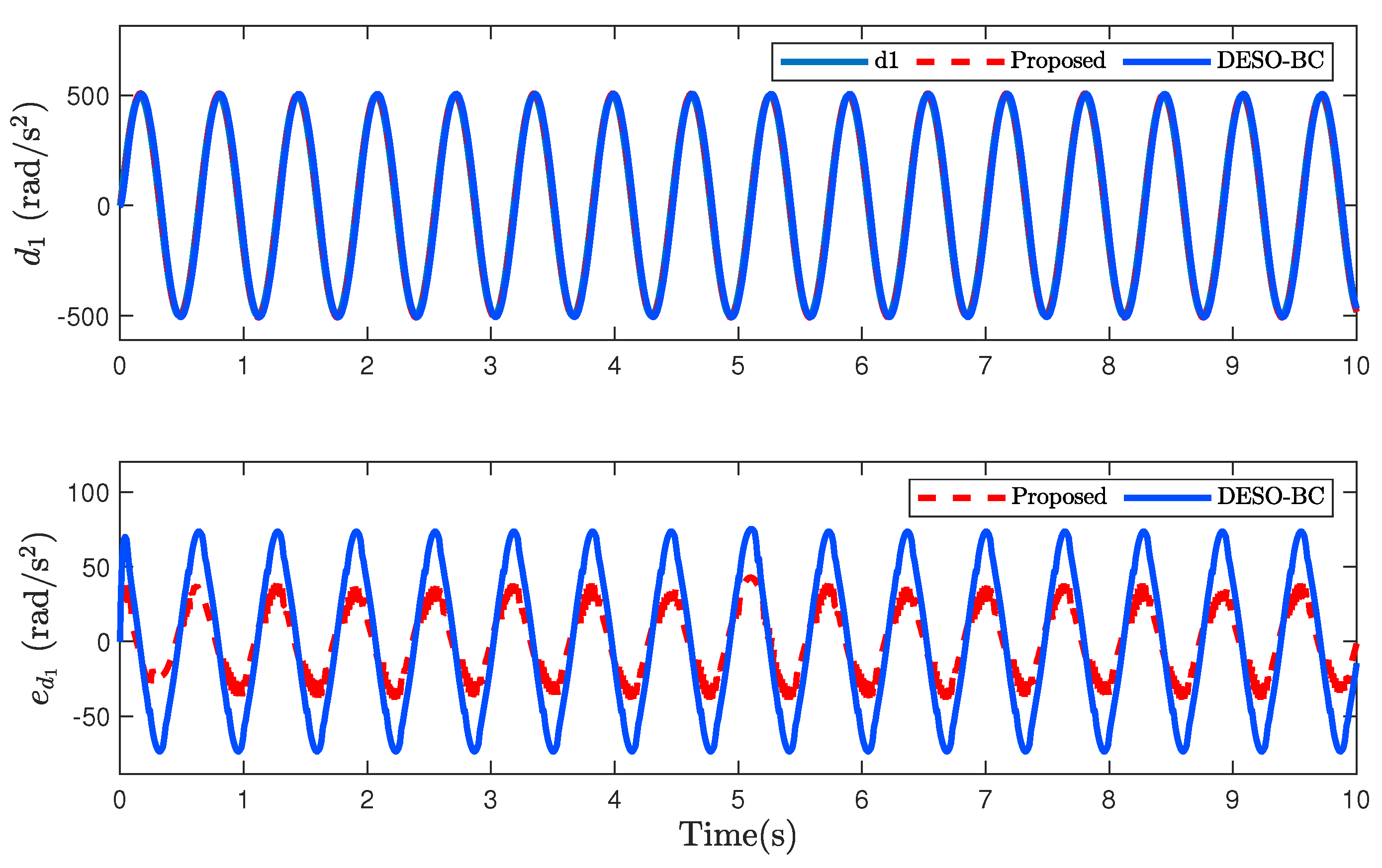
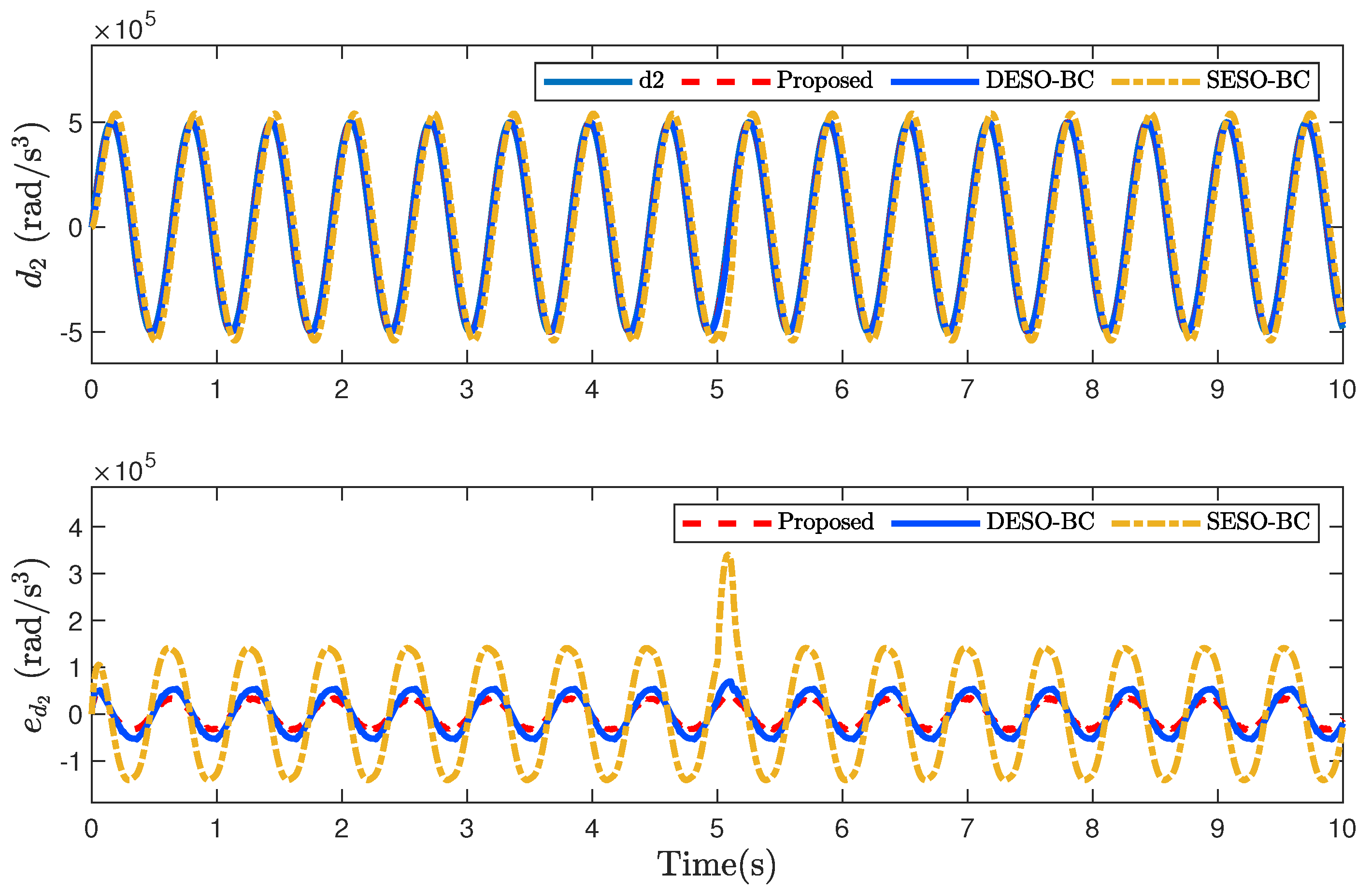
Proposed control strategy with controller gains as $k_1=350$, $k_2=250$, $k_3=150$. The bandwidths of the designed ESMO and ESO are chosen as ${\omega }_1=450$ and ${\omega }_2=450$, respectively. The time constant of filters is $T_f=0.001$. For the trajectory planner, its parameters are selected based on the system specifications as ${\ddot{x}}_{1d}^{+}=40$, ${\ddot{x}}_{1d}^{-}=-40$, ${\dot{x}}_{1d}^{+}=30$, ${\dot{x}}_{1d}^{-}=-30$, $C_{tp}={10}^5$, and $T=0.001$.

(2)

DESO-BC (Dual Extended State Observer-based Command Filtered Backstepping Controller): Without the integration of PPC, the control structure and controller parameters are chosen as same as the proposed controller. The two ESOs [52] are designed to simultaneously estimate the angular velocity and both lumped mismatched and matched uncertainties, and their bandwidths are picked as ${\omega }_1=450$ and ${\omega }_2=450$.

(3)

SESO-BC (Single Extended State Observer-based Command Filtered Backstepping Controller): The output feedback controller is constructed based on command filtered backstepping control (CF-BSC) framework, whose control architecture and controller gains are designed equivalent to the DESO-BC controller. In this control scheme, an ESO [44] is established to estimate immeasurable angular velocity, load pressure, and lumped matched uncertainty with the bandwidth of the ESO is $\omega =450$.

To examine the robustness of the three control approaches, the time-varying lumped mismatched and matched disturbances $d_1\left(t\right)$ and $d_2\left(t\right)$ are purposely inserted into the control system as

$$\begin{array}{cc}\hfill & d_1\left(t\right)=500\sin (\pi t/2)(\mathrm{rad}/{\mathrm{s}}^2)\hfill \\ \hfill & d_2\left(t\right)=5\times {10}^5\sin (\pi t/2)(\mathrm{rad}/{\mathrm{s}}^3)\hfill \end{array}$$

(60)

Performance indexes in the steady-state regime including the maximum, average, and standard deviation of the tracking errors [44] are used to measure the tracking qualifications of the above controllers. These terms are given by:

(1)

Maximal absolute tracking error

$$M_e=\underset{i=1,\dots ,N}{max}\left\{\left|{ϵ}_1\left(i\right)\right|\right\}$$

(61)

where ${ϵ}_1$ is the output tracking error and N denotes the number of samples.

(2)

Average tracking error

$${\mu }_e=\frac{1}{N}\sum _{i=1}^N\left|{ϵ}_1\left(i\right)\right|$$

(62)

(3)

Standard deviation of the tracking errors

$${\sigma }_e=\sqrt{\frac{1}{N}\sum _{i=1}^N{\left(\left|{ϵ}_1\left(i\right)\right|-{\mu }_e\right)}^2}$$

(63)

4.2. Case Study 1: Non-Smooth Reference Trajectory

Firstly, the three controllers are tested with the reference trajectory (in radian unit) which has the following form

$$x_{1d}\left(t\right)=\left\{\begin{array}{ccc}0,\hfill & \mathrm{if}& t<5\mathrm{s}\\ \pi /\phantom{\pi 8,}8,\hfill & \mathrm{if}& t\ge 5\mathrm{s}\end{array}\right.$$

(64)

The tracking performances of all controllers are illustrated in Figure 5. To clearly demonstrate the tracking capabilities of all controllers in the steady-state regime, two zoom-in figures in the top-left region (from the 1st second to 3rd second) and bottom-left region (from the 7th second to 9th second) of Figure 5 are given. As shown, the proposed control strategy possesses the smallest tracking error during these periods. Meanwhile, due to the lack of the mismatched disturbance compensation mechanism, the SESO-BC controller performs the worst with the largest tracking error. In addition, regarding the transient performances of all controllers, it can be seen from the sub-figure (from the 4.8th second to the 5.5th second) in the bottom right corner of this figure that although the proposed control method exhibits the longest transient time compared to the DESO-BC and SESO-BC controllers, the smallest overshoot is achieved by the recommended controller.

Moreover, the original reference trajectory is smoothened by the designed nonlinear filter-based trajectory planner (32) and (33), hence, the recommended approach guarantees the prescribed tracking performance as depicted in Figure 6 even when the desired trajectory changes abruptly and under the influences of the lumped mismatched and matched disturbances on the mechanical part and hydraulic dynamic. The predefined time-varying tracking performance is given by $\rho \left(t\right)=(\pi /4-0.002)e^{-10t}+0.002$, $\underline{\upsilon }=1$, and $\overline{\upsilon }=1$. It should be emphasized that only the tracking-error curve of the proposed controller produced by the deviations between the system output and customized reference trajectory is given for fair comparison since the remaining controllers completely cannot fulfill the prescribed performance in the case of step desired trajectory.

The performance indexes of all controllers in the steady-state are given in

Table 2. Performance indexes of all controllers in the case of step reference trajectory in the steady-state regime.

Controller	${\mathit{M}}_{\mathit{e}}$ (rad)	${\mathit{\mu }}_{\mathit{e}}$ (rad)	${\mathit{\sigma }}_{\mathit{e}}$ (rad)
Proposed	$7.5795\times {10}^{-4}$	$4.7642\times {10}^{-4}$	$2.0903\times {10}^{-4}$
DESO-BC	$23.0193\times {10}^{-4}$	$15.3353\times {10}^{-4}$	$7.0569\times {10}^{-4}$
SESO-BC	$57.6372\times {10}^{-4}$	$38.8567\times {10}^{-4}$	$17.4823\times {10}^{-4}$

. It should be noted that the recommended control approach outperforms the remaining controllers in terms of all performance indexes. Specifically, the DESO-BC and SESO-BC controllers violate the output tracking error constraint with the maximal absolute tracking errors being $23.0193\times {10}^{-4}$ (rad) and $57.6372\times {10}^{-4}$ (rad), respectively. Meanwhile, this index attained by the suggested controller is only $7.5795\times {10}^{-4}$ (rad). The better results are obtained by the suggested controller in terms of the remainder indexes. It indicates the effectiveness of the recommended control framework in the disturbance attenuation ability and tracking capability.

The control actions generated by all controllers are demonstrated in Figure 7. It can be seen from this figure that due to the influences of disturbances on system dynamics, the non-zero control actions are always generated to compensate for their effects to maintain the HRA at the desired position. Furthermore, it should be mentioned that when the reference trajectory suddenly varies at the 5th second, because of the lack of the trajectory planner, the SESO-BC controller and DESO-BC controller must produce much higher control efforts to track the step reference trajectory. On the contrary, since the filtered reference trajectory is smooth, a remarkably less control endeavor is required to ensure the predefined tracking performance. The results indicate that the trajectory planner plays an important role in reducing the tracking overshoot and the control effort and achieving the prescribed tracking qualification. Additionally, adopting a trajectory planner can be considered as an effective way to avoid the critical input saturation problem which naturally exists in real applications.

The estimation performances of angular velocity and both lumped unmatched and matched disturbances are presented in Figure 8, Figure 9 and Figure 10, respectively. As shown in Figure 8 and Figure 9, with a similar bandwidth, the constructed ESMO can estimate the velocity and lumped mismatched uncertainties more accurately compared to the well-known ESO, hence, better disturbance rejection capability is attained by the proposed control approach. Although the SESO-BC possesses the cost-effectiveness by employing position sensor only, due to the nonexistence of mismatched disturbance estimation and compensation mechanism, the SESO-BC control approach exhibits the worst estimation performances of immeasurable angular velocity and lumped matched disturbance. Therefore, the overall tracking ability of SESO-BC controller is considerably deteriorated compared to the remaining control approaches.

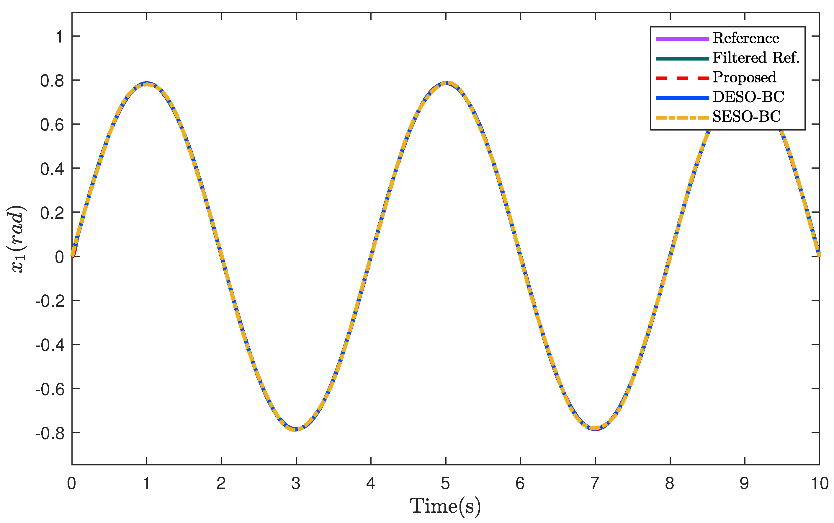
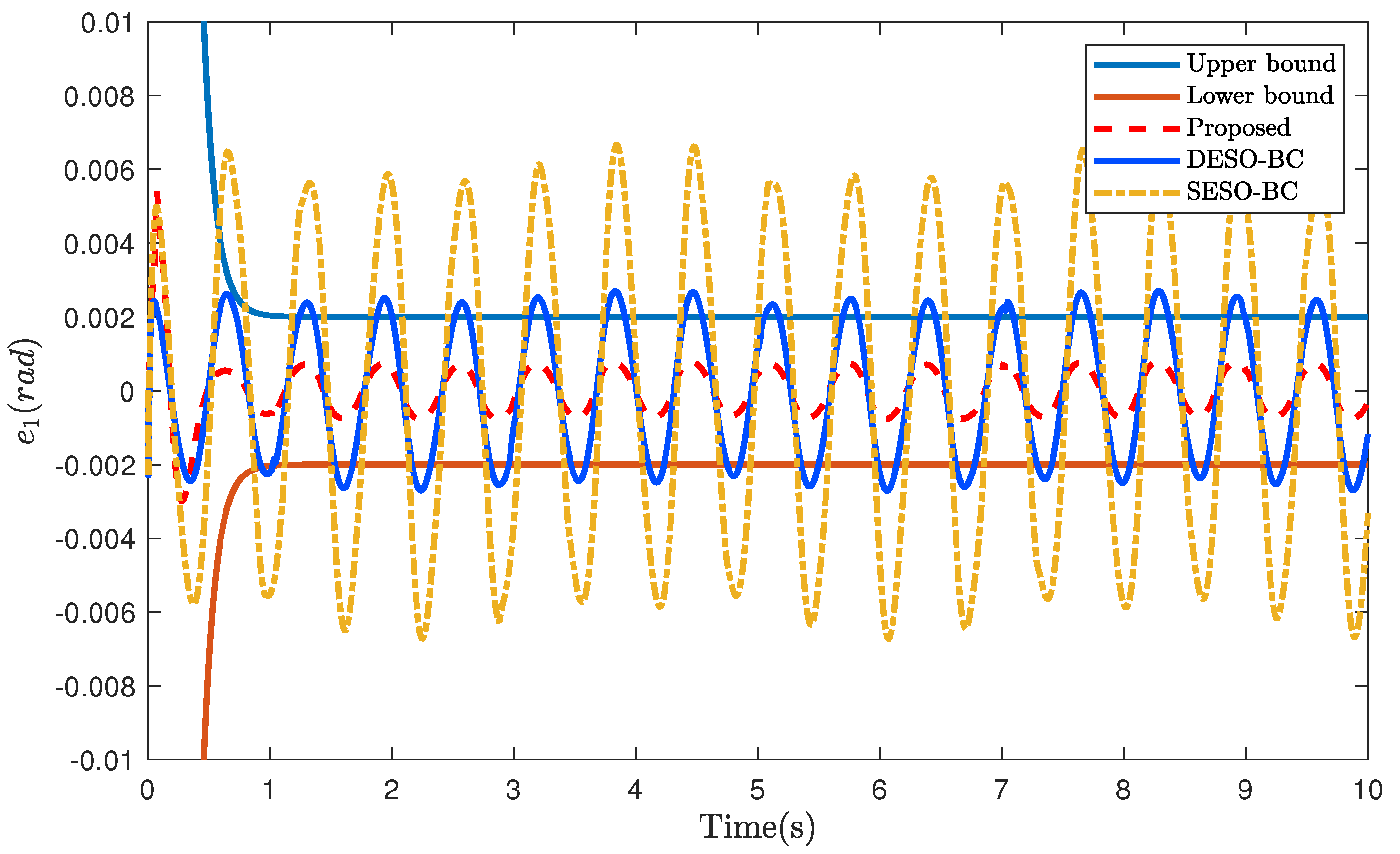
4.3. Case Study 2: Smooth Reference Trajectory

To further examine the effectiveness of the proposed control method, a sinusoidal reference trajectory is employed as $x_{1d}\left(t\right)=\frac{\pi }{4}\sin (\pi t/2)$ (rad). The time-varying prescribed performance function is kept as same as in the above case study. As shown in Figure 11, by virtue of disturbance compensations, all control approaches can track the reference trajectory consistently in spite of the effects of disturbances on the system dynamics. Nonetheless, the DESO-BC and SESO-BC controllers violate the predefined output tracking error constraints as illustrated in Figure 12. Meanwhile, the proposed controller with the PPC mechanism is still able to guarantee the smallest tracking error and satisfy these constraints. It is worth noting that the mismatched and matched disturbances on the control system are estimated more exactly by the combination of the ESMO and ESO and then effectively suppressed by the proposed method, consequently.

The tracking performance indexes of all controllers are provided in

Table 3. Performance indexes of all controllers in the case of the smooth reference trajectory.

Controller	${\mathit{M}}_{\mathit{e}}$ (rad)	${\mathit{\mu }}_{\mathit{e}}$ (rad)	${\mathit{\sigma }}_{\mathit{e}}$ (rad)
Proposed	$7.7322\times {10}^{-4}$	$5.0029\times {10}^{-4}$	$2.2030\times {10}^{-4}$
DESO-BC	$27.1048\times {10}^{-4}$	$16.4598\times {10}^{-4}$	$7.7958\times {10}^{-4}$
SESO-BC	$67.3774\times {10}^{-4}$	$39.7416\times {10}^{-4}$	$18.6279\times {10}^{-4}$

. Similar to the step reference trajectory case study, the suggested control strategy performs better in terms of all performance indexes with smaller values of the maximal absolute tracking error, average tracking error, and standard deviation compared to the remainder control approaches. The results indicate tracking ability and robustness of the proposed method in the presence of disturbances and the nonexistence of velocity measurement mechanism.

Through the two case studies, it can be observed that the proposed control method can be considered as a valuable solution to achieve the predefined performance for tracking control of the EHSs subject to parameter deviations, modeling errors, and unknown external disturbances. In this control scheme, the trajectory planner can be separately designed to ensure that the filtered trajectory is feasible since it takes the kinematic constraints into account. Based on that the input saturation problem is actively avoided and the high-accuracy tracking performance can be achieved. In terms of estimation qualification, compared to the well-known ESO design which is widely adopted in the literature, the ESMO exhibits a higher estimation accuracy. Besides, the PPC is skillfully integrated into the CF-BSC control framework to guarantee that the system output is able to track the desired trajectory with the prescribed convergence rate, overshoot, and steady-state error. However, the predefined performance should be carefully selected to avoid the singularity problem which may cause unexpected issues and should be sufficiently considered in real applications.

5. Conclusions

In this paper, a novel active disturbance rejection control framework was proposed to achieve a high-accuracy prescribed tracking performance for EHSs without velocity measurement mechanism in the presence of both lumped mismatched and matched disturbances caused by parameter deviations, modeling errors, and unknown external loads. To precisely approximate the angular velocity and these disturbances, dual observers, i.e., an ESMO and an ESO, were established. In addition, a trajectory planner considering the kinematics constraints of the EHSs inherited from [19] with minor alterations was constructed to customize the original step reference trajectory, which ensures that the modified reference trajectory always commences at the origin, tracks the original in finite-time, and is sufficiently smooth. Moreover, the integration of the PPC into the CF-BSC based on the designed dual observers and trajectory planner guaranteed that the “explosion of complexity” of the traditional backstepping was effectively avoided and the predefined tracking performances were attained. The stability of the observers and closed-loop control system was rigorously proven by Lyapunov theory. The numerical simulation results showed that the recommended control framework ensures the smallest tracking errors in comparison with other CF-BSC approaches based on well-known ESO design in both cases of the smooth and non-smooth reference trajectories. Parametric uncertainties and time-varying constraints on kinematics and dynamics of the EHS will be deliberately considered in future works.

References

1. Ding, R.; Zhang, J.; Xu, B.; Cheng, M. Programmable hydraulic control technique in construction machinery: Status, challenges and countermeasures. Autom. Constr. 2018, 95, 172–192. [Google Scholar] [CrossRef]
2. Sun, C.; Fang, J.; Wei, J.; Hu, B. Nonlinear Motion Control of a Hydraulic Press Based on an Extended Disturbance Observer. IEEE Access 2018, 6, 18502–18510. [Google Scholar] [CrossRef]
3. Yang, X.; Deng, W.; Yao, J. Neural Adaptive Dynamic Surface Asymptotic Tracking Control of Hydraulic Manipulators with Guaranteed Transient Performance. IEEE Trans. Neural Netw. Learn. Syst. 2022, 2022, 1–11. [Google Scholar] [CrossRef] [PubMed]
4. Yang, H.; Xu, Y.; Chen, Z.; Wang, W.; Aung, N.Z.; Li, S. Cavitation suppression in the nozzle-flapper valves of the aircraft hydraulic system using triangular nozzle exits. Aerosp. Sci. Technol. 2021, 112, 106598. [Google Scholar] [CrossRef]
5. Xu, Z.; Qi, G.; Liu, Q.; Yao, J. ESO-based adaptive full state constraint control of uncertain systems and its application to hydraulic servo systems. Mech. Syst. Signal Process. 2022, 167, 108560. [Google Scholar] [CrossRef]
6. Nguyen, M.H.; Dao, H.V.; Ahn, K.K. Active Disturbance Rejection Control for Position Tracking of Electro-Hydraulic Servo Systems under Modeling Uncertainty and External Load. Actuators 2021, 10, 20. [Google Scholar] [CrossRef]
7. Nguyen, M.H.; Dao, H.V.; Ahn, K.K. Adaptive Robust Position Control of Electro-Hydraulic Servo Systems with Large Uncertainties and Disturbances. Appl. Sci. 2022, 12, 794. [Google Scholar] [CrossRef]
8. Mintsa, H.A.; Venugopal, R.; Kenne, J.-P.; Belleau, C. Feedback Linearization-Based Position Control of an Electrohydraulic Servo System with Supply Pressure Uncertainty. IEEE Trans. Control. Syst. Technol. 2012, 20, 1092–1099. [Google Scholar] [CrossRef]
9. Phan, V.D.; Vo, C.P.; Dao, H.V.; Ahn, K.K. Actuator Fault-Tolerant Control for an Electro-Hydraulic Actuator Using Time Delay Estimation and Feedback Linearization. IEEE Access 2021, 9, 107111–107123. [Google Scholar] [CrossRef]
10. Feng, H.; Song, Q.; Ma, S.; Ma, W.; Yin, C.; Cao, D.; Yu, H. A new adaptive sliding mode controller based on the RBF neural network for an electro-hydraulic servo system. ISA Trans. 2022. [Google Scholar] [CrossRef]
11. Zou, Q. Extended state observer-based finite time control of electro-hydraulic system via sliding mode technique. Asian J. Control 2021, 2021, 1–17. [Google Scholar] [CrossRef]
12. Yang, X.; Deng, W.; Yao, J. Disturbance-observer-based adaptive command filtered control for uncertain nonlinear systems. ISA Trans. 2022. [Google Scholar] [CrossRef] [PubMed]
13. Li, C.; Lyu, L.; Helian, B.; Chen, Z.; Yao, B. Precision Motion Control of an Independent Metering Hydraulic System with Nonlinear Flow Modeling and Compensation. IEEE Trans. Ind. Electron. 2022, 69, 7088–7098. [Google Scholar] [CrossRef]
14. Yang, X.; Ge, Y.; Deng, W.; Yao, J. Adaptive dynamic surface tracking control for uncertain full-state constrained nonlinear systems with disturbance compensation. J. Frankl. Inst. 2022, 359, 2424–2444. [Google Scholar] [CrossRef]
15. Yuan, M.; Chen, Z.; Yao, B.; Hu, J. An Improved Online Trajectory Planner with Stability-Guaranteed Critical Test Curve Algorithm for Generalized Parametric Constraints. IEEE/ASME Trans. Mechatr. 2018, 23, 2459–2469. [Google Scholar] [CrossRef]
16. Kim, J.; Croft, E.A. Online near time-optimal trajectory planning for industrial robots. Robot.-Comput.-Integr. Manuf. 2019, 58, 158–171. [Google Scholar] [CrossRef]
17. Luo, X.; Li, S.; Liu, S.; Liu, G. An optimal trajectory planning method for path tracking of industrial robots. Robotica 2019, 37, 502–520. [Google Scholar] [CrossRef]
18. Lan, J.; Xie, Y.; Liu, G.; Cao, M. A Multi-Objective Trajectory Planning Method for Collaborative Robot. Electronics 2020, 9, 859. [Google Scholar] [CrossRef]
19. Gerelli, O.; Bianco, C.G.L. Nonlinear Variable Structure Filter for the Online Trajectory Scaling. IEEE Trans. Ind. Electron. 2009, 56, 3921–3930. [Google Scholar] [CrossRef]
20. Swaroop, D.; Hedrick, J.K.; Yip, P.P.; Gerdes, J.C. Dynamic surface control for a class of nonlinear systems. IEEE Trans. Autom. Control. 2000, 45, 1893–1899. [Google Scholar] [CrossRef] [Green Version]
21. Guo, Q.; Li, X.; Jiang, D. Full-State Error Constraints Based Dynamic Surface Control of Electro-Hydraulic System. IEEE Access 2018, 6, 53092–53101. [Google Scholar] [CrossRef]
22. Guo, Q.; Shi, G.; Wang, D. Adaptive Composite Fuzzy Dynamic Surface Control for Electro-Hydraulic-System, with Variable-Supply-Pressure. Asian J. Control. 2020, 22, 521–535. [Google Scholar] [CrossRef]
23. Liu, S.; Hao, R.; Zhao, D.; Tian, Z. Adaptive Dynamic Surface Control for Active Suspension with Electro-Hydraulic Actuator Parameter Uncertainty and External Disturbance. IEEE Access 2020, 8, 156645–156653. [Google Scholar] [CrossRef]
24. Zhang, X.; Shi, G. Dual extended state observer-based adaptive dynamic surface control for a hydraulic manipulator with actuator dynamics. Mech. Mach. Theory 2022, 169, 104647. [Google Scholar] [CrossRef]
25. Farrell, J.A.; Polycarpou, M.; Sharma, M.; Dong, W. Command Filtered Backstepping. IEEE Trans. Autom. Control. 2009, 54, 1391–1395. [Google Scholar] [CrossRef]
26. Xie, H.; Tang, Y.; Shen, G.; Li, X.; Bai, D.; Sa, Y. Command filtered adaptive backstepping control for high-accuracy motion tracking of hydraulic systems with extended state observer. Proc. Inst. Mech. Eng. Part J. Syst. Control. Eng. 2022, 236, 654–668. [Google Scholar] [CrossRef]
27. Hao, R.; Wang, H.; Liu, S.; Yang, M.; Tian, Z. Multi-objective command filtered adaptive control for nonlinear hydraulic active suspension systems. Nonlinear Dyn. 2021, 105, 1559–1579. [Google Scholar] [CrossRef]
28. Ren, H.; Deng, G.; Hou, B.; Wang, S.; Zhou, G. Finite-Time Command Filtered Backstepping Algorithm-Based Pitch Angle Tracking Control for Wind Turbine Hydraulic Pitch Systems. IEEE Access 2019, 7, 135514–135524. [Google Scholar] [CrossRef]
29. Kanchanaharuthai, A.; Mujjalinvimut, E. Fixed-time command-filtered backstepping control design for hydraulic turbine regulating systems. Renew. Energy 2022, 184, 1091–1103. [Google Scholar] [CrossRef]
30. Wang, S.; Ren, X.; Na, J.; Zeng, T. Extended-State-Observer-Based Funnel Control for Nonlinear Servomechanisms with Prescribed Tracking Performance. IEEE Trans. Autom. Sci. Eng. 2017, 14, 98–108. [Google Scholar] [CrossRef]
31. Guo, G.; Li, D. Adaptive Sliding Mode Control of Vehicular Platoons with Prescribed Tracking Performance. IEEE Trans. Veh. Technol. 2019, 68, 7511–7520. [Google Scholar] [CrossRef]
32. Wang, M.; Yang, A. Dynamic Learning From Adaptive Neural Control of Robot Manipulators with Prescribed Performance. IEEE Trans. Syst. Man Cybern. Syst. 2017, 47, 2244–2255. [Google Scholar] [CrossRef]
33. Zhang, R.; Xu, B.; Zhao, W. Finite-time prescribed performance control of MEMS gyroscopes. Nonlinear Dyn. 2020, 101, 2223–2234. [Google Scholar] [CrossRef]
34. Ho, C.M.; Tran, D.T.; Nguyen, C.H.; Ahn, K.K. Adaptive Neural Command Filtered Control for Pneumatic Active Suspension with Prescribed Performance and Input Saturation. IEEE Access 2021, 9, 56855–56868. [Google Scholar] [CrossRef]
35. Xu, Z.; Liu, Q.; Yao, J. Adaptive prescribed performance control for hydraulic system with disturbance compensation. Int. Adapt. Control. Signal Process. 2021, 35, 1544–1561. [Google Scholar] [CrossRef]
36. Xu, Z.; Wang, Y.; Shen, H.; Liu, Q.; Yao, J. Funnel function-based asymptotic output feedback control of hydraulic systems with prescribed performance. IET Control Theory Appl. 2021, 15, 2271–2285. [Google Scholar] [CrossRef]
37. Guo, Q.; Zhang, Y.; Celler, B.G.; Su, S.W. Neural Adaptive Backstepping Control of a Robotic Manipulator with Prescribed Performance Constraint. IEEE Trans. Neural Netw. Learn. Syst. 2019, 30, 3572–3583. [Google Scholar] [CrossRef]
38. Guo, Q.; Liu, Y.; Jiang, D.; Wang, Q.; Xiong, W.; Liu, J.; Li, X. Prescribed Performance Constraint Regulation of Electrohydraulic Control Based on Backstepping with Dynamic Surface. Appl. Sci. 2018, 8, 76. [Google Scholar] [CrossRef] [Green Version]
39. Huang, H.; He, W.; Li, J.; Xu, B.; Yang, C.; Zhang, W. Disturbance Observer-Based Fault-Tolerant Control for Robotic Systems with Guaranteed Prescribed Performance. IEEE Trans. Cybern. 2022, 52, 772–783. [Google Scholar] [CrossRef]
40. Yang, Y.; Li, Y.; Liu, X.; Huang, D. Adaptive neural network control for a hydraulic knee exoskeleton with valve deadband and output constraint based on nonlinear disturbance observer. Neurocomputing 2022, 473, 14–23. [Google Scholar] [CrossRef]
41. Won, D.; Kim, W.; Shin, D.; Chung, C.C. High-Gain Disturbance Observer-Based Backstepping Control with Output Tracking Error Constraint for Electro-Hydraulic Systems. IEEE Trans. Control. Syst. Technol. 2015, 23, 787–795. [Google Scholar] [CrossRef]
42. Yao, Z.; Liang, X.; Zhao, Q.; Yao, J. Adaptive disturbance observer-based control of hydraulic systems with asymptotic stability. Appl. Math. Model. 2022, 105, 226–242. [Google Scholar] [CrossRef]
43. Han, J. From PID to Active Disturbance Rejection Control. IEEE Trans. Ind. Electron. 2009, 56, 900–906. [Google Scholar] [CrossRef]
44. Yao, J.; Jiao, Z.; Ma, D. Extended-State-Observer-Based Output Feedback Nonlinear Robust Control of Hydraulic Systems with Backstepping. IEEE Trans. Ind. Electron. 2014, 61, 6285–6293. [Google Scholar] [CrossRef]
45. Luo, C.; Yao, J.; Gu, J. Extended-state-observer-based output feedback adaptive control of hydraulic system with continuous friction compensation. J. Frankl. Inst. 2019, 356, 8414–8437. [Google Scholar] [CrossRef]
46. Zhang, J.; Shi, P.; Lin, W. Extended sliding mode observer based control for Markovian jump linear systems with disturbances. Automatica 2016, 70, 140–147. [Google Scholar] [CrossRef]
47. Woldegiorgis, A.T.; Ge, X.; Li, S.; Hassan, M. Extended Sliding Mode Disturbance Observer-Based Sensorless Control of IPMSM for Medium and High-Speed Range Considering Railway Application. IEEE Access 2019, 7, 175302–175312. [Google Scholar] [CrossRef]
48. Liu, J.; Vazquez, S.; Wu, L.; Marquez, A.; Gao, H.; Franquelo, L.G. Extended State Observer-Based Sliding-Mode Control for Three-Phase Power Converters. IEEE Trans. Ind. Electron. 2017, 64, 22–31. [Google Scholar] [CrossRef] [Green Version]
49. Ke, D.; Wang, F.; He, L.; Li, Z. Predictive Current Control for PMSM Systems Using Extended Sliding Mode Observer with Hurwitz-Based Power Reaching Law. IEEE Trans. Power Electron. 2021, 36, 7223–7232. [Google Scholar] [CrossRef]
50. Yu, J.; Sun, Y.; Lin, W.; Li, Z. Fault-tolerant control for descriptor stochastic systems with extended sliding mode observer approach. IET Control Theory Appl. 2017, 11, 1079–1087. [Google Scholar] [CrossRef]
51. Dao, H.V.; Ahn, K.K. Extended Sliding Mode Observer-Based Admittance Control for Hydraulic Robots. IEEE Robot. Autom. Lett. 2022, 7, 3992–3999. [Google Scholar] [CrossRef]
52. Yao, J.; Deng, W. Active Disturbance Rejection Adaptive Control of Hydraulic Servo Systems. IEEE Trans. Ind. Electron. 2017, 64, 8023–8032. [Google Scholar] [CrossRef]
53. Merritt, H.E. Hydraulic Control Systems; J. Wiley: Hoboken, NJ, USA, 1967. [Google Scholar]
54. Deng, W.; Yao, J.; Wang, Y.; Yang, X.; Chen, J. Output feedback backstepping control of hydraulic actuators with valve dynamics compensation. Mech. Syst. Signal Process. 2021, 158, 107769. [Google Scholar] [CrossRef]
Figure 1. The studied electro-hydraulic system configuration. (a) The architecture of the EHS control system; (b) The hydraulic circuit of the considered EHS.
Applsci 12 06034 g001
Figure 2. The proposed control scheme.
Applsci 12 06034 g002
Figure 3. The structure of the nonlinear filter-based trajectory planner.
Applsci 12 06034 g003
Figure 4. An example of the prescribed time-varying tracking performance with ρ 0 = 1 , ρ = 0.03 , υ ¯ = 1 , υ ̲ = 1 , and ϕ = 10 .
Applsci 12 06034 g004
Figure 5. Tracking performances of all controllers in case of step reference trajectory.
Applsci 12 06034 g005
Figure 6. Tracking performance of the suggested controller in case of step reference trajectory.
Applsci 12 06034 g006
Figure 7. Control actions of all control approaches in case of step reference trajectory.
Applsci 12 06034 g007
Figure 8. Angular velocity estimation performances of all control approaches in case of step reference trajectory.
Applsci 12 06034 g008
Figure 9. Lumped mismatched uncertainty estimation performances of all control approaches in case of step reference trajectory.
Applsci 12 06034 g009
Figure 10. Lumped matched uncertainty estimation performances of all control approaches in case of step reference trajectory.
Applsci 12 06034 g010
Figure 11. Tracking performances of all controllers in case of sinusoidal reference trajectory.
Applsci 12 06034 g011
Figure 12. Tracking errors of all controllers in case of sinusoidal reference trajectory.
Applsci 12 06034 g012