Defect Recognition and Morphology Operation in Binary Images Using Line-Scanning-Based Induction Thermography

Abstract

Active infrared thermography is an attractive and highly reliable technique used for the non-destructive evaluation of test objects. In this paper, defect detection on the subsurface of the STS304 metal specimen was performed by applying the line-scanning method to induction thermography. In general, the infrared camera and the specimen are fixed in induction thermography, but the line-scanning method can excite a uniform heat source because relative movement occurs. After that, the local heating area due to Joule’s heating effect was removed, and filtering was applied for the 1st de-noising. Threshold-value-based binarization processing using the Otsu algorithm was performed for clear defect object recognition. After performing the 2nd de-noising, automatic defect recognition was performed using a boundary tracking algorithm. As a result, the conditions due to the parameters of the scanning line for the thermal image were determined.

1. Introduction

Non-destructive testing (NDT) is the performance of an inspection without destroying an object [1]. As a representative example, when using steel materials, such as bridges, railways, structures, and pipes, to join metals together, most are welded, and various inspection techniques are used to inspect the soundness of the welded area without physically affecting these metal joints [2]. In other words, NDT measures changes in the properties and characteristics of applied energy due to the presence of defects by excitation with physical energy (sunlight, heat, radiation, ultrasound, and electricity) without changing the originality and function of the material [3,4,5]. It means an inspection to determine the presence or absence of defects by measuring through equipment.

There are numerous metal materials that are widely used in industrial fields, and stainless steel (STS) is typically used [6,7]. STS contains more than 12% chromium and is not easily rusted, so it is a material used in various fields such as industrial parts, automobile parts, medical devices, and aerospace fields. However, due to various causes (fatigue damage, manufacturing defects, corrosion, etc.), defects occur on the surface or inside, which can lead to serious problems due to weak durability. Therefore, many NDT techniques are used to perform on-site inspections. An inspection for on-site maintenance requires promptness, safety, and reliability. Recently, infrared thermography (IRT) that meets these conditions is emerging as an advanced technology [8].

IRT is a technology that has developed rapidly in recent years and utilizes IR camera microsystem technology that integrates an IR detector, electronic technology, and computer technology [9,10,11]. IRT analysis is currently being applied to industry and R&D in various fields such as NDT inspection, condition monitoring and diagnosis, predictive maintenance, energy saving in the process and construction fields, and the detection of gas components.

Among NDT inspection techniques, IRT is mainly used to detect defects, discontinuities, delaminations, and welding defects inside objects [2]. IRT is a technology that analyzes and acquires a thermal response signal using a non-contact-method-based thermal imager. After providing a heat source to the object to be inspected with an external thermal excitation source, the IR camera detects radiant energy belonging to the IR range of the electromagnetic spectrum. Based on this principle, it is possible to detect internal abnormalities [12,13,14]. NDT techniques for discontinuous points existing inside an inspection object are very diverse.

Table 1. Summary of representative classifications in NDT techniques.

Reference Citation	Method Used	Target Material	Sensor Used	Calculation Method	Performance Metric	Limitations
[15]	Capacitive Imaging	CFRP	Coplanar capacitive sensor	Serial intensity	Contrast comparative	Local detection of defect,
[16]				Intensity analysis	Qualitative Evaluation	Defect detection on surface or thin layers
[17]	Pulsed active thermography	Buried anti-personnel mines	FLIR T 650 SC thermal camera	Circular Hough transformation	Accuracy	Reduced detectability of binarized images due to low resolution
[18]	Feature extraction	Fabric defects	-	Feature extraction, Machine learning	Accuracy, Precision	Low accuracy of surface defects compared to time calculation
[19]	Ultrasonic Testing	CFRP	Phased array transducer	Phased array (PA)	Quantitative Evaluation	Requires a lot of data to improve accuracy
[20]	Inductive Thermography	Steel	IR camera	Image segmentation	Precision, Recall	Reduced detectability due to noise
[21]	Vibrothermography	ASTM E399-05 compact tension specimen	SC3000 IR Camera	Heat capacity by frictional heating	High sensitivity and accuracy inspection for micro-cracks	Inspection of localized surface cracks

presents various NDT techniques for examining the discontinuous points of an inspection object.

For all NDT techniques, an appropriate technique should be selected according to the type and defect of the inspection object. The STS304 plate applied in this study has circular defects of various aspect ratios on the back side, so an inspection technique that can inspect non-contact or large areas and acquire high-level quantitative data is required. The capacitive imaging (CI) technique is advantageous for detecting local defects present in thin layers or surfaces, so it is advantageous for detecting composite materials such as CFRP or GFRP. Ultrasonic testing (UT) can acquire quantitative data of defects but is performed with local detection and contact. Vibrothermography (VT) is suitable for tensile specimens in which cracks are present and there is a potential for defect growth due to frictional vibrations.

Various image processing techniques are used to improve the detectability of the 2D thermal images acquired with an infrared camera or to detect defects automatically. Recently, machine learning is used, but a lot of data accumulation is required. In addition, noise may be generated by non-uniform heat sources when optical or electromagnetic techniques are used, and noise can be minimized in the binarized image compared to the study in [20].

Active IRT technology can be broadly classified into three types: optical, electromagnetic, and mechanical. The optical method uses a halogen lamp or a flash lamp as an external heat source to perform inspection [2]. It has the advantage of having a periodic heat source in the form of a sine wave or providing instantaneous pulse energy to the object to be inspected and being able to inspect a wide area. However, it has a limitation in that noise is generated in the 2D thermal image due to non-uniform heat source excitation [22].

The mechanical method measures the frictional heat of the microcracks in an object to be inspected with an infrared camera through ultrasonic excitation [21,23]. When the probe is in direct contact with an object to transmit ultrasound, there is a risk that microcracks may grow or break. Since heat must be generated by friction, it can be applied only to crack-type defects. In addition, general infrared cameras have a low resolution, which makes quantitative analysis difficult, so a high-performance camera is required.

The electromagnetic method is a technique of inducing an electric current in an object to be inspected after forming a magnetic field around it by flowing an electric current through a coil [24]. This technique enables uniform heat source excitation and the inspection of various types of defects. However, this is only possible for magnetic materials, and in the case of the static mode, the inspection object and coil are measured together by the infrared camera, which may affect the detectability [25,26]. Therefore, in this paper, in order to overcome the limitations of the electromagnetic method, a moving mode in which the relative motion of the specimen and the infrared camera occurs was utilized, and a process for acquiring sequence images was performed.

In this paper, the detection of subsurface defects in the STS304 specimen was performed using the electromagnetic induction thermography technique. Induction thermography, also called eddy current thermography (ECT), is a technique of inducing electromagnetic waves to inspect objects using an excitation coil. Due to the inherent problems previously described for the other techniques and in order to overcome the limitations of the electromagnetic method, a new method was devised. In this paper we employed a moving mode in which the relative motion of the specimen and the IR camera occurred, and a process for acquiring sequence images was performed.

The remainder of the paper is composed as follows. In Section 2, the numerical theory of induction thermography and the principle of LSM are explained. In Section 3, the schematic diagram of the STS304 specimen with circular defects on the back side that was used in this study and the configuration diagram of the induction thermography devices are described. In addition, the image processing of the 2D thermal data acquired from the experiment are described. Section 4 presents the experimental data on which image processing was performed, and a comparative analysis is performed by citing data obtained from the LIT in the references. Finally, Section 5 concludes the paper.

2. Theory

2.1. Mathematical Theory

When a high-frequency alternating current flows through the induction coil, an eddy current is induced in the surrounding metal (conductor). The penetration depth of the eddy current is closely related to the properties of the metal and the excitation frequency, and the penetration depth equation for this is as follows [27,28,29]:

$$\mathsf{\delta }=\frac{1}{\sqrt{\mathsf{\pi }\mathsf{\sigma }\mathsf{\mu }\mathrm{f}}}$$

(1)

where $\mathsf{\delta }$ is the penetration depth, $\mathsf{\sigma }$ is the electrical conductivity, $\mathsf{\mu }$ is permeability, and $\mathrm{f}$ is the excitation frequency. The penetration depth of eddy currents has a characteristic inversely proportional to the electrical conductivity, magnetic permeability, and excitation frequency.

If the eddy current passes through the discontinuity after induced in the metal, the density of the current changes, as shown in Figure 1. In the region where the eddy current density is increased, a high level of Joule’s heating occurs, and the equation for this is as follows:

$${\mathrm{q}}_{\mathrm{s}}={\left|\mathrm{J}\right|}^2/\mathsf{\sigma }$$

(2)

where ${\mathrm{q}}_{\mathrm{s}}$ is the intensity of the heat power and $\mathrm{J}$ is the density of the current. In the case of induction thermography, the effect on $\mathsf{\sigma }$ is negligible because the change with respect to temperature is relatively small, so it can be regarded as a constant.

The heat generated by the eddy current propagates inside the metal specimen, and the equation for this is as follows [30]:

$${\mathsf{\rho }\mathrm{c}}_{\mathrm{p}}\frac{\partial \mathrm{T}}{\partial \mathrm{t}}+{\mathsf{\rho }\mathrm{c}}_{\mathrm{p}}\mathrm{u}·\nabla \mathrm{T}=\nabla ·\left(\mathrm{k}\nabla \mathrm{T}\right)+{\mathrm{q}}_{\mathrm{s}}$$

(3)

where $\mathsf{\rho }$ is the density, ${\mathrm{c}}_{\mathrm{p}}$ is the specific heat, $\mathrm{T}$ is the temperature, $\mathrm{t}$ is the time, $\mathrm{k}$ is the heat transfer coefficient, and $\mathrm{u}$ is the dynamic speed of the metal.

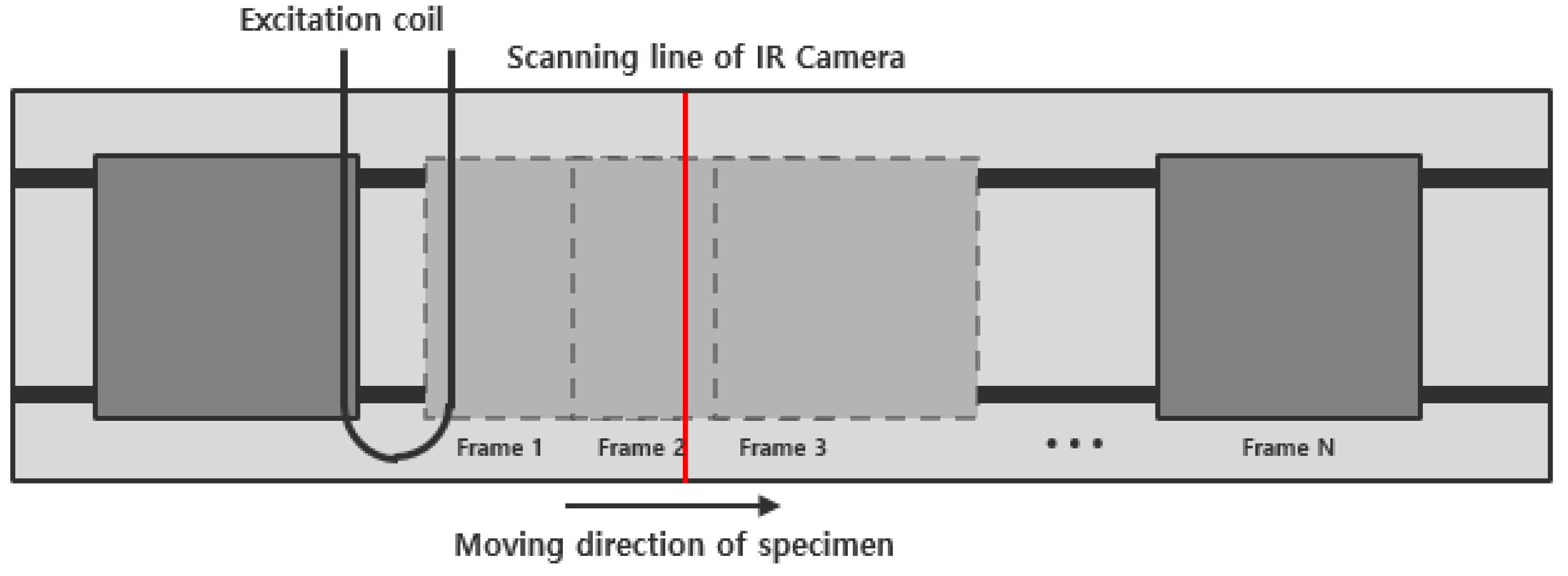
2.2. Line-Scanning Method

In general, induction thermography is performed in a static mode where relative motion does not occur between the specimen and the IR camera. If the experiment is performed in a static mode, the shape of the coil is measured as it is in the 2D thermal image acquired with an IR camera, which may become an obstacle to defect detection. Therefore, to solve this problem, the device was designed so that movement occurs between the specimen and the IR camera. Figure 2 shows the principle of the line-scanning technique [31]. The specimen moves along the sliding guide rail, and the image is acquired by setting the scanning line in the FLIR software dedicated to the IR camera [32,33].

By applying LSM to induction thermography, it is possible to provide a uniform heat source to the specimen. In the case of lock-in infrared thermography (LIT) or pulsed infrared thermography (PT), which are widely used among active infrared thermography techniques, a lamp is used to provide a heat source. This provides a non-uniform heat source to the surface of the specimen, causing a lot of noise. For this reason, the LSM has the advantage of significantly improving the detectability by providing a uniform heat source and generating relatively little noise [34,35].

3. Experimental Setup

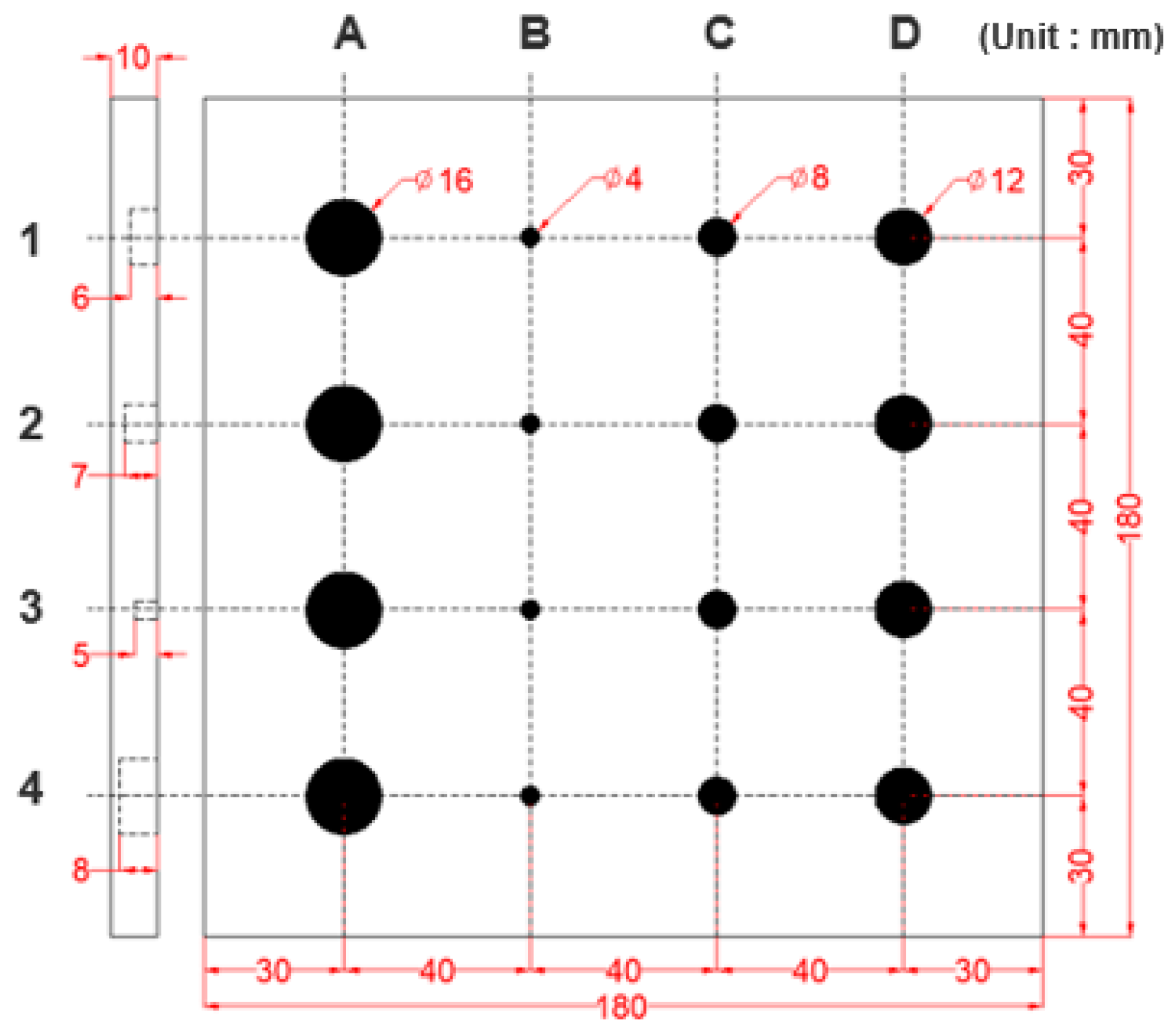
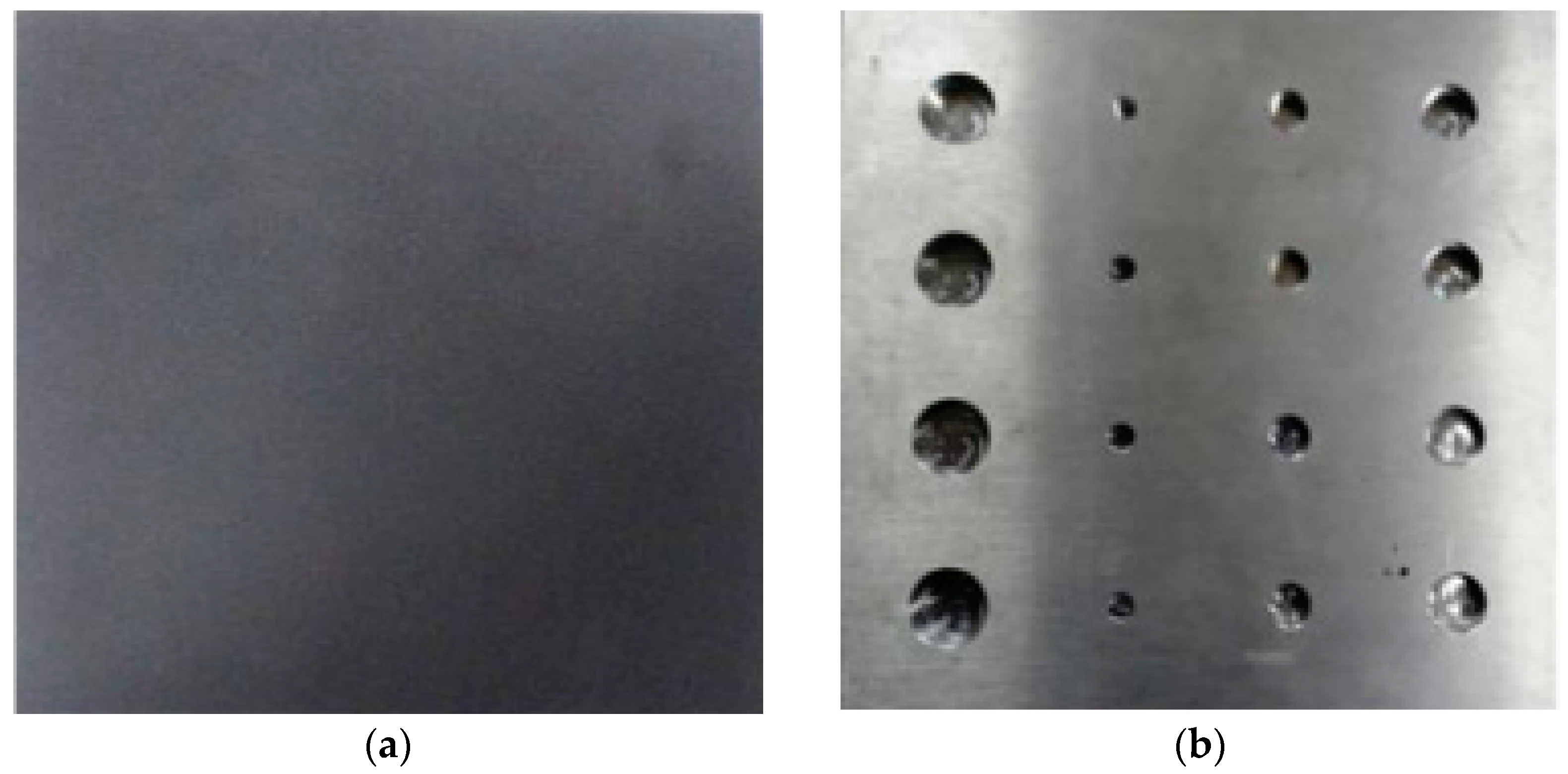
3.1. STS304 Reference Specimen

The specimen used in the induction thermography experiment was the STS304 reference specimen provided by the Korea Research Institute of Standards and Science (KRISS) in Korea. On the backside, there are artificial defects of various sizes and diameters. As shown in Figure 3, the diameter is the same horizontally and the depth is the same vertically. It is square in shape and has a thickness of 10 mm and dimensions of 180 $\times$ 180 mm. There are a total of 16 circular defects, and each defect is indexed with a unique symbol. The defects on the column axis are indexed as 1, 2, 3, and 4, and the defects on each row axis are indexed as A, B, C, and D. For example, the deepest defect with the largest diameter is indexed as ‘A4′. The surface of the specimen was coated with Krylon’s black paint in order to maintain an emissivity of 0.95 or more. Figure 4 shows the front and back sides of the specimen, and

Table 2. The material properties of the STS304 specimen.

Thermal Conductivity (k)	16.2 W/m·K
Electrical Conductivity	106 Siemens/m
Density	8000 kg/m3
Heat Capacity	500 J/kg·K
Initial Temperature	23 °C

shows the physical properties of STS304.

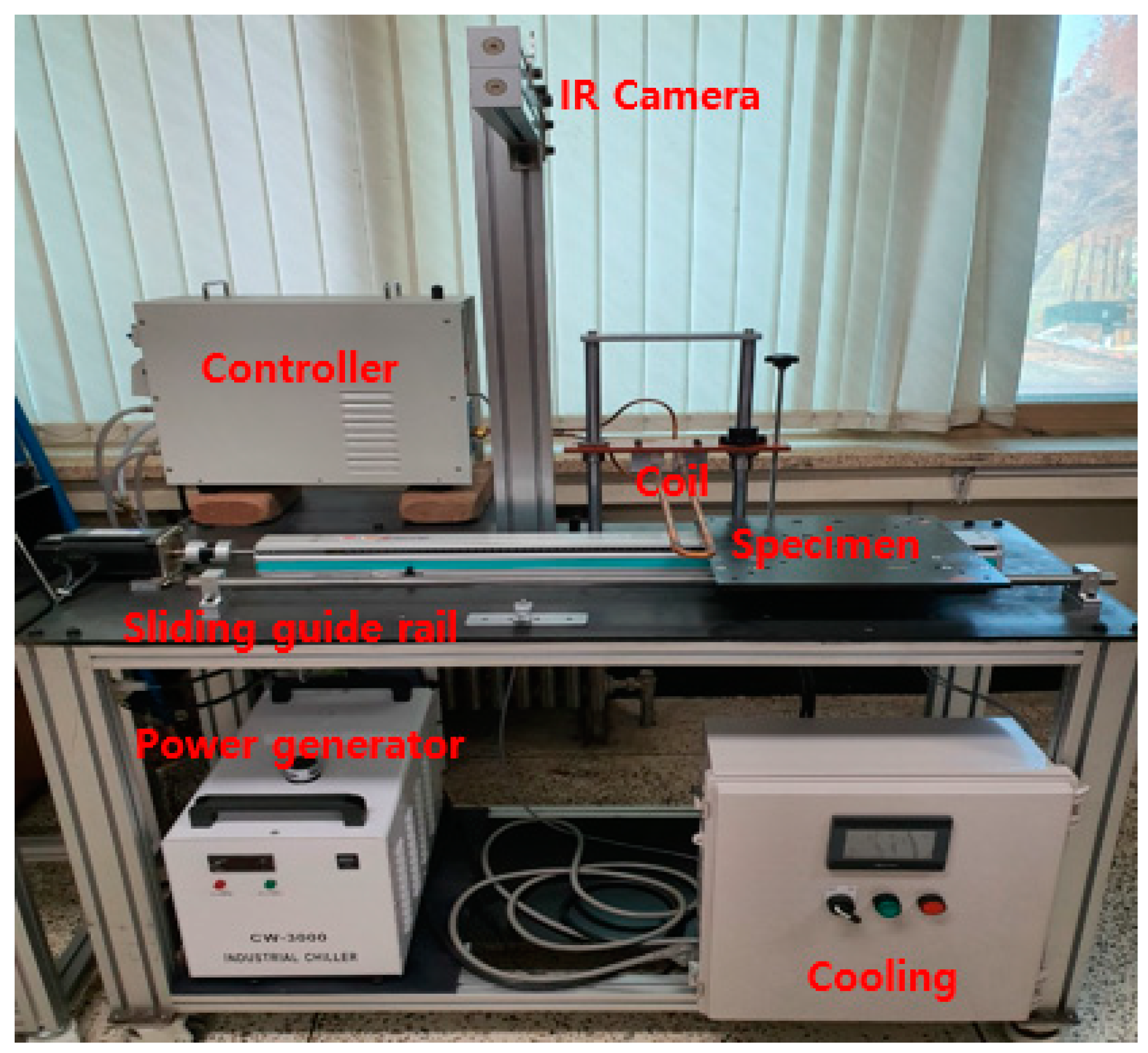
3.2. LSM Configuration

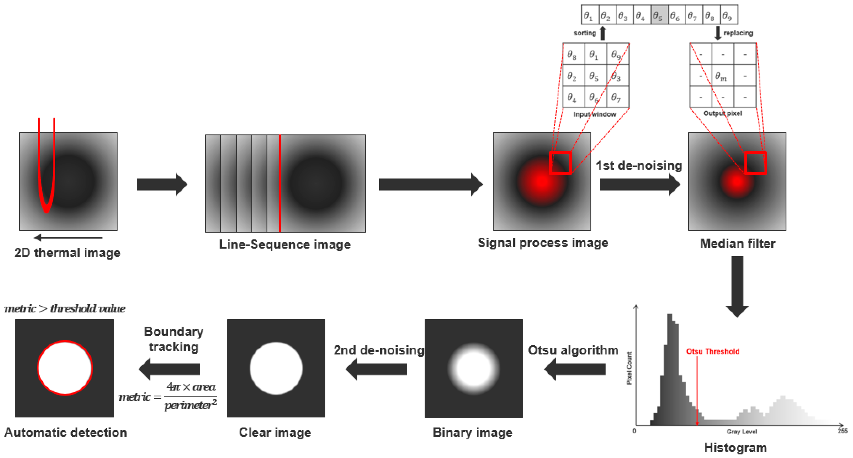
In this study, an experiment was performed in which the LSM was applied to induction thermography, and Figure 5 shows the experimental configuration. The material of the excitation coil for heating the specimen was copper and was manufactured in a ‘U’ type. For the measurement of the surface of the specimen, where heat is generated due to the induction coil, a long-wavelength FLIR SC645 model (un-cooled type, 640 $\times$ 480 pixels, 7.5~13 $\mathsf{\mu }\mathrm{m}$) IR camera was used. The IR camera was placed vertically at a distance of 600 mm from the specimen. The maximum output of the power supply was 15 kW. The excitation current was set to 135 A, the frequency of the alternating current was set at 40 kHz, and the speed was set to 5 mm/s, 10 mm/s, 15 mm/s, and 20 mm/s. As the speed of the specimen moving along the slide guide was slow, the amount of heat source supplied to the specimen increased, which is a very important factor because it determines the thermal contrast of the 2D thermal image. The image frame rate and lift-off were set to 50 Hz and 2 mm, respectively, where lift-off means the distance between the specimen and the copper coil. The cooling device in Figure 6 played a role in cooling the high temperature of the copper coil while the current was excited, and the excitation current was controlled by a controller and a power generator. The images acquired with the IR camera were post-processed through a PC.

3.3. Image Process

Figure 7 shows the image processing flow of the 2D thermal image acquired by applying LSM to the induction thermography in this study. The detailed process for each step was as follows:

Step 1:

In order to provide a uniform heat source to the surface of the specimen, a 2D thermal image was acquired by applying LSM to induction thermography.

Step 2:

After calculating the total frame for the 2D scanning image, the thermal image for a specific frame was extracted. In general, the scanning line selected the starting point for the visual identification of the specimen as the infrared camera monitored the moving specimen. After that, a sequence image for a specific frame was acquired based on the scanning line, and the image was cropped using the crop function to analyze the area of the specimen in the entire image.

Step 3:

Filtering (mean, median, Gaussian, and NLmeans) was applied to the cropped raw image for the 1st de-noising, and the SNR of the ROI was calculated for a comparative analysis of detectability.

Step 4:

In order to classify clear defect objects in the image, binarization was performed using the Otsu algorithm, and the 2nd de-noising was performed.

Step 5:

Using the boundary tracking function, the automatic defect recognition in the image was performed based on the threshold value through the roundness equation, and the error rate was analyzed for reliability verification.

4. Results and Discussion

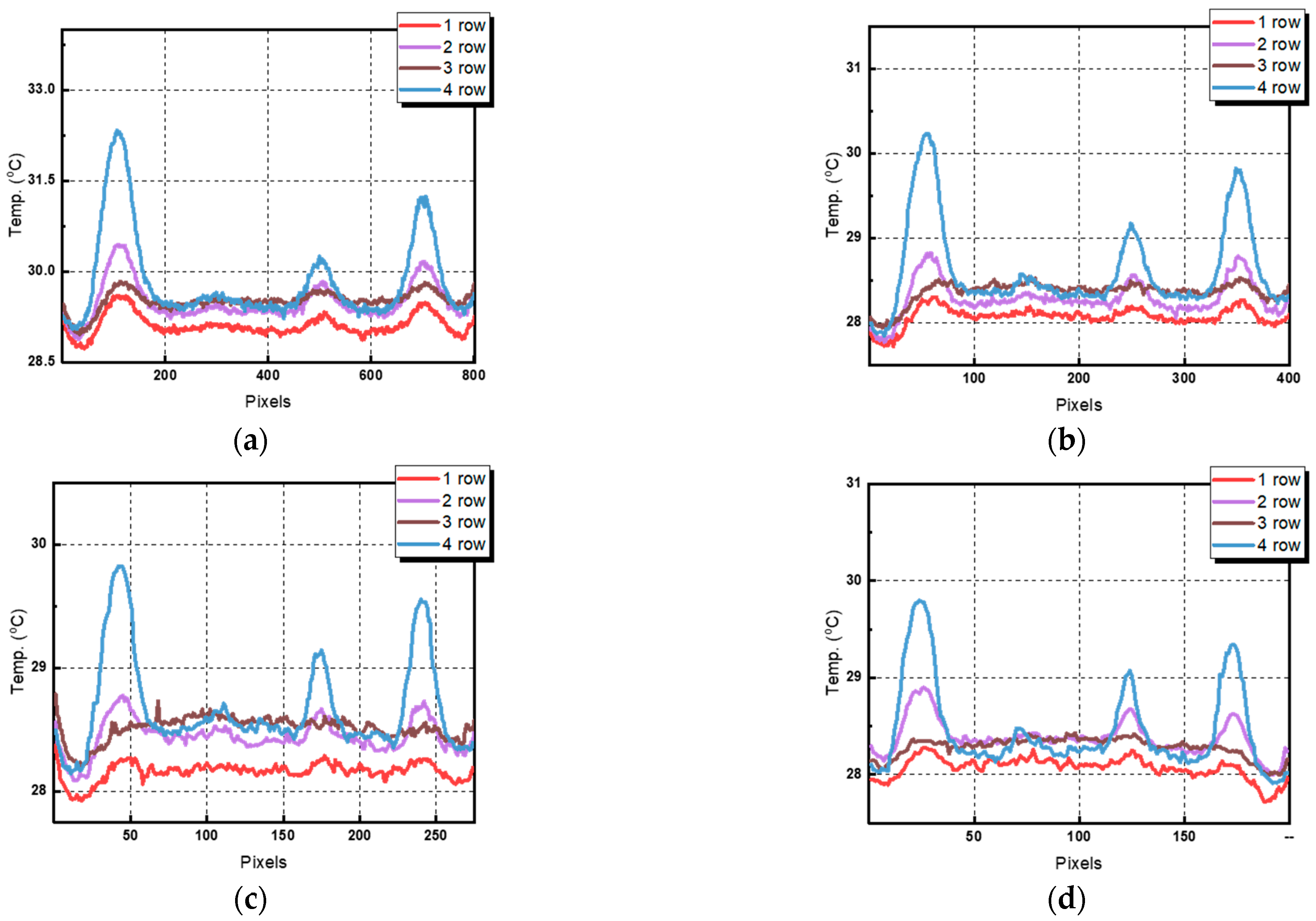
4.1. Two-Dimensional Thermal Image

Heat was provided to the surface of the specimen with an excitation coil, and a 2D thermal image, measured with an IR camera, was acquired. The images for total frames were loaded into MATLAB software using LSM. After acquiring a sequence image based on the scanning line, only the image area of the specimen was cropped using the ‘crop’ function. If the crop was not performed, even coils appeared in the image and became an obstacle to image processing.

As the moving speed of the specimen was slower, the amount of heat source supplied increased, and it can be seen in Figure 8a that the temperature was relatively high. When there was a large supply of a heat source, the temperature of the whole specimen improved. Therefore, the thermal profile of each row was analyzed to compare the thermal contrast between the defective area and the sound area, as shown in Figure 9.

The slower the moving speed of the specimen, the greater the input amount of the heat source supplied to the surface. This increased the overall temperature of the specimen. However, as the input amount of the heat source increased, the thermal contrast between the defective area and the sound area did not increase. Therefore, the process of determining the optimal thermal contrast (a high thermal contrast between the defective area and the sound area means that the detectability is improved) was performed. Two ROIs of 5 $\times$ 5 pixels (one at the center of the defective area and another in the adjacent sound area) were set for the defective area and the sound area. The thermal contrast equation is as follows [36]:

$$\Delta \mathrm{c}={\mathrm{DROI}}_{\mathrm{mean}}-{\mathrm{SROI}}_{\mathrm{mean}}$$

(4)

where ${\mathrm{DROI}}_{\mathrm{mean}}$ and ${\mathrm{SROI}}_{\mathrm{mean}}$ mean the average temperatures of the defective area and sound area, respectively.

Table 3. The value of the thermal contrast between the defective area and sound area.

Moving Speed	Thermal Contrast
5 mm/s	2.41 °C
10 mm/s	1.52 °C
15 mm/s	1.04 °C
20 mm/s	0.89 °C

shows the average thermal contrast values for the four defects in the four rows for each moving speed. It can be seen that the largest thermal contrast occurred at 5 mm/s. Although it was not linearly proportional, it can be considered that the slower the moving speed, the greater the amount of heat supplied so that the thermal contrast is larger.

4.2. Filtering for 1st De-Noising

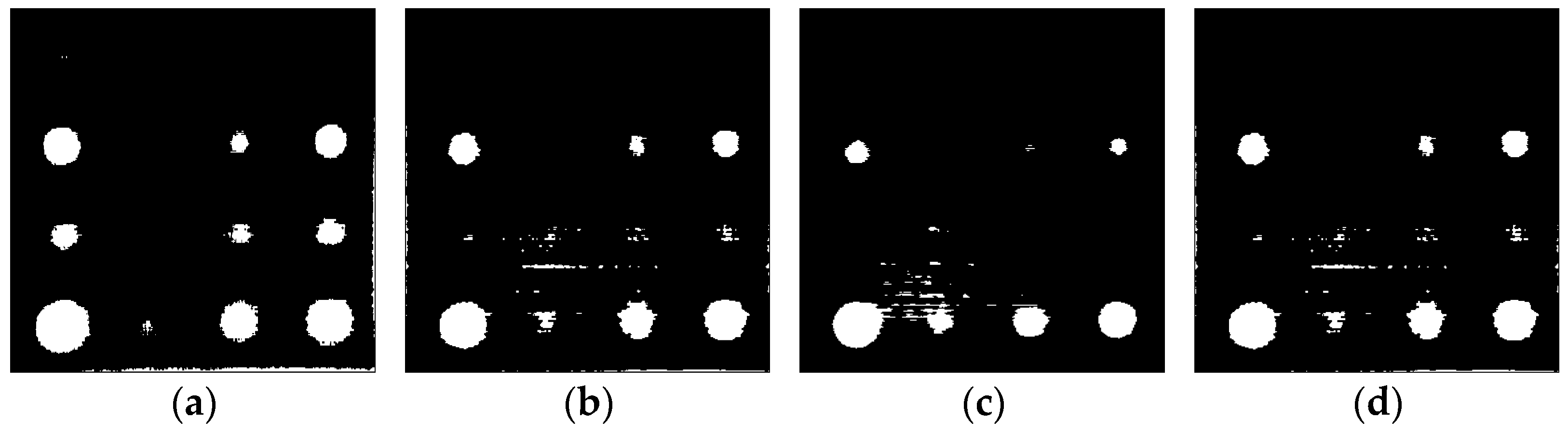
After analyzing the optimal thermal contrast in the 2D image for each moving speed, a process was performed to improve the detectability. For the 1st de-noising, four types of filtering were applied to the image [37,38,39]. Figure 10 shows the non-filtered raw image and the filtered image for 5 mm/s, where the thermal contrast was the largest.

To compare and analyze the detectability of each filtered image, the signal-to-noise ratio (SNR) was calculated. The SNR is defined as the ratio between the signal area and the background noise, where the signal area is defined as a defective part and the noise area is defined as a sound area. The selected ROI area was a defect whose index signature was A4. The SNR equation is as follows [40]:

$$\mathrm{SNR}=20{\log }_{10}\left(\frac{\left|{\mathrm{DROI}}_{\mathrm{mean}}-{\mathrm{SROI}}_{\mathrm{mean}}\right|}{\mathsf{\sigma }}\right)$$

(5)

where ${\mathrm{DROI}}_{\mathrm{mean}}$ and ${\mathrm{SROI}}_{\mathrm{mean}}$ are the arithmetic means of all the pixels in defective area and sound area, respectively, and $\mathsf{\sigma }$ is the standard deviation of all the pixels the sound area.

Table 4. The value of the SNR for each filtering image.

Filter Type	SNR
	5 mm/s	10 mm/s	15 mm/s	20 mm/s
Raw (non-filtering)	38.5549	35.4555	25.8822	27.1765
Median	54.6857	39.0084	29.1514	33.3562
Mean	50.9123	38.6698	37.7273	39.4107
Gaussian	33.6764	36.1395	32.6425	33.4680
NLmeans	35.7586	36.2160	34.7896	13.4450

shows the SNR values for all filtered images for each moving speed. Overall, the SNR values were improved in the filtered images compared to the raw image (non-filtering). In addition, based on the 5 mm/s image with the highest SNR improvement, it can be seen that the SNR of LIT was significantly improved after the 1st de-noising presented in [18] was applied. For 5 mm/s and 10 mm/s, median filtering effectively improved the detectability, and for 15 mm/s and 20 mm/s, mean filtering, effectively improved the detectability. Moreover, median filtering and mean filtering can be applied faster than Gaussian filtering and NLmeans filtering because their calculation methods are simple. In fact, although the performance of each PC was different, they were possible to calculate within seconds. After that, binarization was performed by applying the Otsu algorithm to the filtered images selected at each moving speed.

4.3. Binary Process

There are many techniques for analyzing images. Among them, the simplest and easiest method is to binarize an image using a threshold value. It is used in many preprocessing steps in image processing, such as separating the background from objects in an image, extracting only pixels with a brightness value above a certain level, or simplifying all the information in an image. The Otsu algorithm is the most representative method for calculating the threshold of an image [20,41,42].

The Otsu algorithm is a method of calculating the optimal threshold for classifying images into two classes using a histogram based on gray scale [43]. In order to classify the image into two classes, an appropriate threshold value, k (where, 0 < k < L − 1), must be calculated. Based on the threshold value, k, in the binarized image, [0, k] is classified as ‘class 1’, and [k + 1, L − 1] is ‘class 2’. Through this process, a binarized image can be obtained. In general, converting a 2D thermal image into a binarized image can clearly characterize the signature of the defect.

In order to classify the two binarized images, it is necessary to calculate the optimal threshold. When there is an M $\times$ N size image having L intensity levels, such as [0, 1, 2, …, L − 1], pixels having intensity values within are classified as class 1, and intensity values within are classified as class 2. The probability that a pixel is classified into ‘class 1’ and ‘class 2’ is as follows:

$${\mathrm{P}}_1\left(\mathrm{k}\right)={\displaystyle \sum }_{\mathrm{i}=0}^{\mathrm{k}}{\mathrm{P}}_{\mathrm{i}}$$

(6)

$${\mathrm{P}}_2\left(\mathrm{k}\right)=1-{\mathrm{P}}_1\left(\mathrm{k}\right)$$

(7)

The average intensity values of the pixels classified into classes 1 and 2 are as follows:

$${\mathrm{m}}_1\left(\mathrm{k}\right)=\frac{1}{{\mathrm{P}}_1\left(\mathrm{k}\right)}{\displaystyle \sum }_{\mathrm{i}=0}^{\mathrm{k}}{\mathrm{iP}}_{\mathrm{i}}$$

(8)

The average intensity values up to the k level among all images are as follows:

$${\mathrm{m}}_{\mathrm{G}}={\mathrm{P}}_1{\mathrm{m}}_1+{\mathrm{P}}_2{\mathrm{m}}_2$$

(9)

To calculate the optimal threshold, the Otsu algorithm must apply the concept of between-class variance, as follows [44]:

$${\mathsf{\sigma }}_{\mathrm{b}}^2=\frac{{\left({\mathrm{m}}_{\mathrm{G}}{\mathrm{P}}_1-\mathrm{m}\right)}^2}{{\mathrm{P}}_1\left(1-{\mathrm{P}}_1\right)}$$

(10)

Calculating the optimal k value is a simple principle, but it can be calculated only by substituting all k values in the intensity range [0, L − 1]. The k value was calculated using MATLAB software, and the principle of the Otsu algorithm is to classify the binarization based on the k value obtained in this way. The Otsu algorithm was applied for the binarization of the image with the highest SNR improvement at each speed, as shown in Figure 11.

In Figure 11, all defects in row 1 were not detected. For this reason, although there was a thermal contrast with the sound area, as shown in Figure 9, it could be seen as a result of the relatively small diameter and shallow depth of the defect.

In the binarized image, even if filtering is applied, it can be confirmed that noise is present. In addition, heat was generated locally due to Joule’s effect on the edge of the image, and it was classified as a light and dark value, similar to a defect. In this case, noise was removed through a morphological operation, and a process of homogenizing defect boundaries was performed for automatic object recognition.

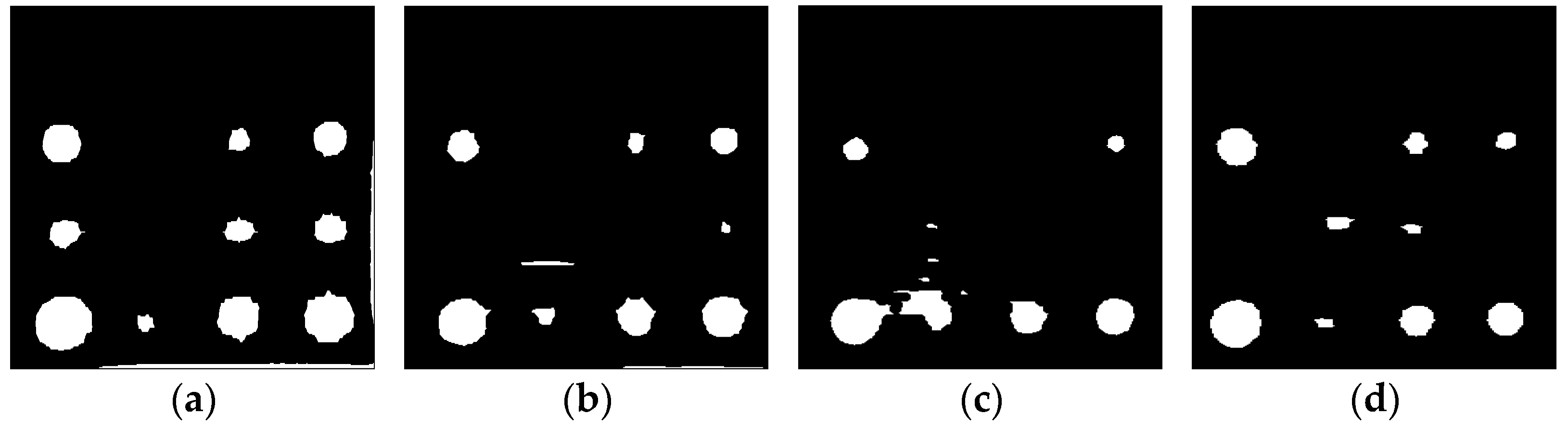
4.4. Morphology for 2nd De-Noising

Morphology is an extensive processing imaging technique that processes images according to the shape of an object. In the morphology operation, each pixel of the image is affected by the values of other nearby pixels, and the size and shape of the neighboring pixels are directly selected to generate a morphology operation sensitive to the specific shape of the image to be input.

The morphological operations performed in this study are as follows: The noise was removed by using the ‘bwareaopen’ function. The object border was homogenized using the disk shape input function of the ‘strel’ function, and the ‘imfill’ function was used to fill the empty spaces of gaps in the object’s pixels. Figure 12 shows the image on which the morphological operation has been performed.

Qualitatively, the most defective object was detected in the 5 mm/s binary image. For this reason, the slower the speed, the more heat that is supplied to the specimen, resulting in a large thermal contrast between the sound area and defective area. Therefore, automatic object recognition was only performed using images of 5 mm/s.

4.5. Automatic Defect Recognition

After the 2nd de-noising was performed, the roundness metric was utilized for automated defect detection. The area and perimeter of each defect were calculated, and the roundness metric equation is as follows [45]:

$$\mathrm{metric}=\frac{4\mathsf{\pi }\times \mathrm{area}}{{\mathrm{perimeter}}^2}$$

(11)

The roundness metric means that the closer to 1, the closer to a circular shape, and it is calculated as the ratio of the object’s perimeter to its area. The threshold value set in this study was 0.75, and defects were recognized based on the threshold value. In addition, if an object was lower than the threshold and it was not recognized as a defect, it was set so that it could be determined by ‘EdgeDetection’. Figure 13 shows the automated defect detection images of the induction thermography performed in this study and the amplitude and phase images acquired using the optical infrared thermography in [24].

A total of 10 defects were detected due to the threshold. All defects in row 1 failed to be detected, and this was because the thermal profile in row 1 in Figure 9 had a relatively small change rate. In addition, it can be confirmed that the effect of Joule’s heating generated on the edge of the STS304 specimen was detected with ‘EdgeDetection’.

Finally, after the 2nd de-noising was performed, the root-mean-square error (RMSE) was calculated to compare the detectability with the LIT technique, and the equation is as follows [46]:

$$\mathrm{RMSE}\left({\mathsf{\theta }}_1,{\mathsf{\theta }}_2\right)=\sqrt{\frac{{{\displaystyle \sum }}_{\mathrm{i}=1}^{\mathrm{n}}{({\mathsf{\theta }}_{1,\mathrm{i}}-{\mathsf{\theta }}_{2,\mathrm{i}})}^2}{\mathrm{n}}}$$

(12)

where ${\mathsf{\theta }}_1$ is real value, ${\mathsf{\theta }}_2$ is estimated value, and n is number of areas. The roundness metric is a dimensionless unit, and the RMSE was calculated as a percentage.

Table 5. Detectability comparative analysis of optical and electromagnetic methods.

Hole	Optical [24]		Electromagnetic
	Amplitude (0.02 Hz)	Phase (0.01 Hz)
A1	-	88	-
A2	87	86	90
A3	81	88	75
A4	86	88	87
B1	-	-	-
B2	-	-	-
B3	-	-	-
B4	-	-	85
C1	-	80	-
C2	81	82	81
C3	79	-	-
C4	83	84	83
D1	-	81	-
D2	88	84	89
D3	92	86	81
D4	92	89	82
RMSE	23.657	23.638	24.565

shows the RMSE values compared with the results of the LIT study conducted in [24].

It can be seen that the defect detectability is slightly inferior to that of the optical technique. The electromagnetic technique has an advantage in that the SNR is relatively significantly improved after filtering is applied because there is little noise due to the uniformity of the heat source. Therefore, when image processing is performed in real time rather than in the form of an image, the electromagnetic technique can be considered suitable.

5. Conclusions and Future Works

In this paper, automatic object recognition research was performed using LSM-based induction thermography. A 2D thermal image was acquired based on the scanning line, and filtering was applied for the 1st de-noising. Based on the SNR value of the raw image (non-filtering) in Table 4, 5 mm/s improved by 41.83%, 10 mm/s improved by 10.02%, 15 mm/s improved by 45.76%, and 20 mm/s improved by 45.01%. After that, for clear defect detection, binarization was performed using the Otsu algorithm, and the 2nd de-noising was performed through a morphological operation. For automatic object recognition, defect detection was performed using the boundary tracking algorithm, and the area generated under the influence of Joule’s heating was completely separated and detected.

After de-noising was performed, a comparative analysis of the detectability of the optical and electromagnetic methods was performed. The efficiency for automatic defect detection was relatively superior to the electromagnetic method, and it is considered to be a suitable technique through real-time image processing in the future. In addition, an important point in defect detection is to establish a mechanism that can be verified using the probability of detection (POD) method with reliability.

References

1. Maldague, X.P. Nondestructive Testing Handbook. Infrared and Thermal Testing; American Society for Nondestructive Testing: Arlingate Lane, OA, USA, 2001; Volume 3. [Google Scholar]
2. Maldague, X.P. Introduction to NDT by Active Infrared Thermography. Mater. Eval. 2002, 60, 1060–1073. [Google Scholar]
3. Choi, M.Y.; Kang, K.S.; Park, J.H.; Kim, W.T.; Kim, K.S. Quantitative determination of a subsurface defect of reference specimen by lock-in infrared thermography. NDT E Int. 2008, 41, 119–124. [Google Scholar] [CrossRef]
4. Chung, Y.J.; Lee, S.J.; Kim, W.T. Latest Advances in Common signal Processing of Pulsed Thermography for Enhanced Detectability: A Review. Appl. Sci. 2021, 11, 12168. [Google Scholar] [CrossRef]
5. Shull, P.J. Nondestructive Evaluation: Theory, Techniques, and Applications; CRC Press: New York, NY, USA, 2002. [Google Scholar]
6. Roberts, M.; Wang, K.; Guzas, E.; Lockhart, P.; Tucker, W. Induction infrared thermography for non-destructive evaluation of alloy sensitization. AIP Conf. Proc. 2019, 2102, 120006. [Google Scholar]
7. Haneef, T.; Lahiri, B.B.; Bagavathiappan, S.; Mukhopadhyay, C.K.; Philip, J.; Rao, B.P.C.; Jayakumar, T. Study of the tensile behavior of AISI type 316 stainless steel using acoustic emission and infrared thermography techniques. J. Mater. Res. Technol. 2015, 4, 241–253. [Google Scholar] [CrossRef] [Green Version]
8. Rodríguez-Martín, M.; Lagüela, S.; González-Aguilera, D.; Martinez, J. Prediction of depth model for cracks in steel using infrared thermography. Infrared Phys. Technol. 2015, 71, 492–500. [Google Scholar] [CrossRef]
9. Bagavathiappan, S.; Lahiri, B.B.; Saravanan, T.; Philip, J.; Jayakumar, T. Infrared thermography for condition monitoring—A review. Infrared Phys. Technol. 2013, 60, 35–55. [Google Scholar] [CrossRef]
10. Usamentiaga, R.; Venegas, P.; Guerediaga, J.; Vega, L.; Molleda, J.; Bulnes, F.G. Infrared thermography for temperature measurement and non-destructive testing. Sensors 2014, 14, 12305–12348. [Google Scholar] [CrossRef] [Green Version]
11. Holland, S.D.; Reusser, R.S. Material evaluation by infrared thermography. Annu. Rev. Mater. Res. 2016, 46, 287–303. [Google Scholar] [CrossRef]
12. Ciampa, F.; Mahmoodi, P.; Pinto, F.; Meo, M. Recent advances in active infrared thermography for non-destructive testing of aerospace components. Sensors 2018, 18, 609. [Google Scholar] [CrossRef] [Green Version]
13. Osornio-Rios, R.A.; Antonino-Daviu, J.A.; de Jesus Romero-Troncoso, R. Recent industrial applications of infrared thermography: A review. IEEE Trans. Ind. Inform. 2018, 15, 615–625. [Google Scholar] [CrossRef]
14. Qu, Z.; Jiang, P.; Zhang, W. Development and application of infrared thermography non-destructive testing techniques. Sensors 2020, 20, 3851. [Google Scholar] [CrossRef] [PubMed]
15. Morozov, M.; Jackson, W.; Pierce, S. Capacitive imaging of impact damage in composite material. Compos. Part B 2017, 113, 65–71. [Google Scholar] [CrossRef] [Green Version]
16. Yin, X.; Hutchins, D. Non-destructive evaluation of composite materials using a capacitive imaging technique. Compos. Part B 2012, 43, 1282–1292. [Google Scholar] [CrossRef]
17. Kılınç, M.; Gözde, H. Detection of buried anti-personnel mines in thermal images by circular hough transformation supported active thermography method. J. Fac. Eng. Archit. Gazi Univ. 2020, 35, 697–707. [Google Scholar]
18. Sec¸kin, A.; Sec¸kin, M. Detection of fabric defects with intertwined frame vector feature extraction. Alex. Eng. J. 2022, 61, 2887–2898. [Google Scholar] [CrossRef]
19. Caminero, M.; García-Moreno, I.; Rodríguez, G.; Chacón, J. Internal damage evaluation of composite structures using phased array ultrasonic technique: Impact damage assessment in CFRP and 3D printed reinforced composites. Compos. Part B 2019, 165, 131–142. [Google Scholar] [CrossRef]
20. Gao, B.; Li, X.; Woo, W.; Tian, G. Physics-Based Image Segmentation Using First Order Statistical Properties and Genetic Algorithm for Inductive Thermography Imaging. IEEE Trans. Image Process. 2018, 27, 2160–2175. [Google Scholar] [CrossRef]
21. Mabrouki, F.; Thomas, M.; Genest, M.; Fahr, A. Frictional heating model for efficient use of vibrothermography. NDT E Int. 2009, 42, 345–352. [Google Scholar] [CrossRef]
22. Hedayatrasa, S.; Poelman, G.; Segers, J.; Van Paepegem, W.; Kersemans, M. Performance of frequency and/or phase modulated excitation waveforms for optical infrared thermography of CFRPs through thermal wave radar: A simulation study. Compos. Struct. 2019, 225, 111177. [Google Scholar] [CrossRef]
23. Renshaw, J.; Chen, J.C.; Holland, S.D.; Thompson, R.B. The sources of heat generation in vibrothermography. NDT E Int. 2011, 44, 736–739. [Google Scholar] [CrossRef] [Green Version]
24. Lee, S.J.; Chung, Y.J.; Ranjit, S.; Kim, W.T. Automated Defect Detection Using Threshold Value Classification Based on Thermographic Inspection. Appl. Sci. 2021, 11, 7870. [Google Scholar] [CrossRef]
25. Li, X.; Gao, B.; Woo, W.L.; Tian, G.Y.; Qiu, X.; Gu, L. Quantitative Surface Crack Evaluation Based on Eddy Current Pulsed Thermography. IEEE Sens. J. 2017, 17, 412–421. [Google Scholar] [CrossRef]
26. Shi, Z.; Xu, X.; Ma, J.; Zhen, D.; Zhang, H. Quantitative Detection of Cracks in Steel Using Eddy Current Pulsed Thermography. Sensors 2018, 18, 1070. [Google Scholar] [CrossRef] [PubMed] [Green Version]
27. Oswald-Tranta, B. Induction thermography for surface crack detection and depth determination. Appl. Sci. 2018, 8, 257. [Google Scholar] [CrossRef] [Green Version]
28. Yang, R.; He, Y.; Gao, B.; Tian, G.Y.; Peng, J. Lateral heat conduction based eddy current thermography for detection of parallel cracks and rail tread oblique cracks. Measurement 2015, 66, 54–61. [Google Scholar] [CrossRef]
29. Abidin, I.Z.; Tian, G.Y.; Wilson, J.; Yang, S.; Almond, D. Quantitative evaluation of angular defects by pulsed eddy current thermography. NDT E Int. 2010, 43, 537–546. [Google Scholar] [CrossRef]
30. Chen, Y.; Xu, Z.; Wu, J.; He, S.; Roskosz, M.; Xia, H.; Kang, Y. A Scanning Induction Thermography System for Thread Defects of Drill Pipes. IEEE Trans. Instrum. Meas. 2021, 71, 3502509. [Google Scholar] [CrossRef]
31. He, M.; Zhang, L.; Li, J.; Zheng, W. Methods for suppression of the effect of uneven surface emissivity of material in the moving mode of eddy current thermography. Appl. Therm. Eng. 2017, 118, 612–620. [Google Scholar] [CrossRef]
32. He, M.; Zhang, L.; Zheng, W.; Feng, W. Crack detection based on a moving mode of eddy current thermography method. Measurement 2017, 109, 119–129. [Google Scholar] [CrossRef]
33. He, M.; Zheng, W.; Li, W.; Zhang, Y. Research on temperature distribution law around crack using the moving mode of eddy current thermography. Infrared Phys. Technol. 2019, 102, 102993. [Google Scholar] [CrossRef]
34. Zhang, X.; Peng, J.; He, K.; Gao, X. Nondestructive inspection of holes with distinct spacing in plate using the moving mode of Induction Thermography. Infrared Phys. Technol. 2022, 122, 104045. [Google Scholar] [CrossRef]
35. Tuschl, C.; Oswald-Tranta, B.; Eck, S. Inductive thermography as non-destructive testing for railway rails. Appl. Sci. 2021, 11, 1003. [Google Scholar] [CrossRef]
36. Ranjit, S.; Kim, W.T. Non-destructive testing and evaluation of materials using active thermography and enhancement of signal to noise ratio through data fusion. Infrared Phys. Technol. 2018, 94, 78–84. [Google Scholar]
37. Tabatabaei, N. Matched-filter thermography. Appl. Sci. 2018, 8, 581. [Google Scholar] [CrossRef] [Green Version]
38. Akram, M.W.; Li, G.; Jin, Y.; Chen, X.; Zhu, C.; Zhao, X.; Aleem, M.; Ahmad, A. Improved outdoor thermography and processing of infrared images for defect detection in PV modules. Sol. Energy 2019, 190, 549–560. [Google Scholar] [CrossRef]
39. Forero-Ramírez, J.C.; Restrepo-Girón, A.D.; Nope-Rodríguez, S.E. Detection of internal defects in carbon fiber reinforced plastic slabs using background thermal compensation by filtering and support vector machines. J. Nondestruct. Eval. 2019, 38, 33. [Google Scholar] [CrossRef]
40. Venegas, P.; Perán, J.; Usamentiaga, R.; de Ocáriz, I.S. Projected thermal diffusivity analysis for thermographic nondestructive inspections. Int. J. Therm. Sci. 2018, 124, 251–262. [Google Scholar] [CrossRef]
41. Dong, X.Y. Review of otsu segmentation algorithm. Adv. Mater. Res. 2014, 989, 1959–1961. [Google Scholar] [CrossRef]
42. Manda, M.P.; Kim, H.S. A fast image thresholding algorithm for infrared images based on histogram approximation and circuit theory. Algorithms 2020, 13, 207. [Google Scholar] [CrossRef]
43. Yang, X.; Shen, X.; Long, J.; Chen, H. An improved median-based Otsu image thresholding algorithm. AASRI Procedia 2012, 3, 468–473. [Google Scholar] [CrossRef]
44. Dong, Y.X. An Improved Otsu Image Segmentation Algorithm. Adv. Mater. Res. 2014, 989, 3751–3754. [Google Scholar] [CrossRef]
45. Takashimizu, Y.; Iiyoshi, M. New parameter of roundness R: Circularity corrected by aspect ratio. Prog. Earth Planet. Sci. 2016, 3, 2. [Google Scholar] [CrossRef] [Green Version]
46. Chung, Y.J.; Ranjit, S.; Lee, S.J.; Kim, W.T. Thermographic inspection of internal defects in steel structures: Analysis of signal processing techniques in pulsed thermography. Sensors 2020, 20, 6015. [Google Scholar] [CrossRef] [PubMed]
Figure 1. The principle of induction thermography.
Applsci 12 06006 g001
Figure 2. The principle of the line-scanning method.
Applsci 12 06006 g002
Figure 3. Schematic illustration of the STS304 plate providing depth and diameter dimensions of each defect.
Applsci 12 06006 g003
Figure 4. Pictures of the specimen used in the study: (a) front side coated with black paint and (b) back side with flat-bottomed holes.
Applsci 12 06006 g004
Figure 5. Experimental configuration of induction thermography.
Applsci 12 06006 g005
Figure 6. Actual experimental devices of induction thermography.
Applsci 12 06006 g006
Figure 7. Flowchart of the overall research process of this study.
Applsci 12 06006 g007
Figure 8. Temperature images from the induction thermography based on LSM: (a) 5 mm/s, (b) 10 mm/s, (c) 15 mm/s, and (d) 20 mm/s.
Applsci 12 06006 g008aApplsci 12 06006 g008b
Figure 9. Thermal profile graphs of rows for each moving speed: (a) 5 mm/s, (b) 10 mm/s, (c) 15 mm/s, and (d) 20 mm/s.
Applsci 12 06006 g009
Figure 10. Image with filtering based on raw image: (a) raw image, (b) median filtering, (c) mean filtering, (d) Gaussian filtering, and (e) NLmeans filtering.
Applsci 12 06006 g010
Figure 11. Binary image with the Otsu algorithm applied: (a) 5 mm/s, (b) 10 mm/s, (c) 15 mm/s, and (d) 20 mm/s.
Applsci 12 06006 g011
Figure 12. Binary image with morphology operation applied: (a) 5 mm/s, (b) 10 mm/s, (c) 15 mm/s, and (d) 20 mm/s.
Applsci 12 06006 g012
Figure 13. Automatic defect detection of binarized images using boundary tracking algorithm, (a) object recognition and edge detection of 5 mm/s, (b) amplitude image, and (c) phase image.
Applsci 12 06006 g013