Passenger Volumes and Dwell Times for Commuter Trains: A Case Study Using Automatic Passenger Count Data in Stockholm

Abstract

This study investigates the relationship between passenger volumes and the frequency and size of dwell times for commuter trains. We use data collected by automatic passenger count systems in Stockholm and show that dwell times often take longer than scheduled. To understand the effect of passenger volumes on delays, we use the frequencies of delays for different passenger volumes and delay sizes. We find that these frequencies differ significantly from a frequency distribution independent of passenger volumes, indicating that passenger volumes have an effect on the frequency of dwell time delays. Neglecting passenger volumes underestimates the frequency of delays in most cases, especially for smaller delays. Although the frequency of dwell time delays increases as passenger volumes increase, the same is not necessarily true for their size. The relationship between passenger volumes and delay sizes is thus non-linear, and it depends on scheduled dwell times. We conclude that small increases in dwell times can result in sharp increases in on-time performance but that only increasing dwell times is not sufficient. Measures to speed up the boarding and alighting process are also necessary.

1. Introduction

The increasing popularity and frequency of trains result in a growing pressure to make optimal use of available capacity and result in better timetable planning practices [1,2]. One of the performance indicators of the efficiency of a railway system is the punctuality of trains [3,4]. Punctuality, along with other indicators such as travel time reliability and travel time predictability, is an important factor for passenger satisfaction [5,6]. The importance of these aspects is also reflected in the value of time. The authors of [7] state that in some cases, passengers tend to value a reduction in travel time variability higher compared to the travel time for the same journey. This statement is reflected in [8], who found the estimated value of travel time reliability to be 1.13 times that of in-vehicle time for train travel. Improving punctuality and travel time reliability can thus help with improving the attractiveness of railways as a mode of transport. The two main processes which influence punctuality in the context of rail travel are run and dwell times. It is the latter of these that is under consideration in the study presented here.

1.1. Dwell Time Delays

Dwell times refer to the time a passenger train is stationary at a station, and the duration is based on the difference between the arrival and departure times [9]. Although dwell time delays are relatively small in isolation, these delays are relevant to this study since they can accumulate to a large portion of delay times for an entire journey [4,10] and can have a similar impact on rail capacity as the maximum running speeds of trains [11]. In terms of quantifying dwell time delays, several indicators have been proposed in the past. The authors of [5], for example, mention the probability of a train arriving with a delay of more than three or nine minutes at the final station. Other studies mention the use of the average size of delays and the standard deviation of arrival times, thus highlighting the central tendency and variance. With regard to the variance in arrival times, the difference between the 90th or 80th percentile and the 50th percentile of the measured arrival times is mentioned in the literature as well [6,12]. Examples specific to dwell times are the use of the mean and standard deviation [13] and the ratio between the mean and 95th percentile of the observed dwell times [10]. Focussing on the duration of dwell times alone is, however, not sufficient to understand the dynamics which lay ground to the rise of dwell time delays, as the dwell process is complicated, and multiple factors interact. In broad terms, dwell times consist of a fixed and a dynamic time element [14]. The fixed time element is defined by the technical elements, such as the time it takes to open and close the doors, and the dynamic element is defined by the time it takes for the passenger exchange to be completed [15]. For an extensive review on how passengers influence dwell times, we refer to [16].

1.2. Collecting Passenger Flow Data

To study the relation between dwell time delays and passenger flows, it is necessary to collect data on passenger volumes, which can be collected in different ways. A commonly used method is the use of manual observations, where observers record the number of boarding and alighting passengers and the dwell time duration [13,17,18,19]. Technological advancements in recent years have opened up other, more automated, data collection methods. An example of such a technological advancement is an automatic passenger count system. Automatic passenger count systems are onboard systems that record the number of boarding and alighting passengers. In addition to registering the number of passengers, such systems record actual dwell times on a more detailed level compared to signalling data. An example of the use of automatic passenger count to study dwell times for trains can be found in [20], which made use of several years of automatic passenger count data from Stockholm to study the influence of passengers on dwell times. Another example is in [21], which divided dwell times into different elements in an attempt to develop a dwell time scheduling model. Their study showed how the speed of boarding and alighting passengers changes during the dwelling process and the importance of the boarding and alighting process on the length of dwell times.

1.3. Dwell Time Delays and Passenger Volumes

Several studies have identified the effect of passenger volumes and movement rates on dwell times. Studying the boarding and alighting movement rate of passengers on Dutch railway stations, Wiggenraad [22] found that boarding and alighting times are typically around one second per passenger when passengers move in a cluster. Individual, or non-clustered, movement rates are slightly higher, taking more than four seconds. The authors of [18] present a linear relationship between dwell times and passenger flows, where dwell time increases as passenger flows increase. The authors of [20] found that dwell times can increase by up to 0.3 s for every additional boarding and 0.4 s for every additional alighting passenger. They [23] also found the dominant factor for passenger service times to be the volumes of boarding and alighting passengers, which increase service time by around 0.8 and 0.9 s per additional passenger, respectively.

The majority of existing dwell time or passenger service time models assume a constant rate for boarding and alighting over the whole passenger service time [23], which is not necessarily the case. The authors of [11], for example, found that boarding and alighting rates are not constant across a group of passengers. A later study indicated that passenger movement rates first increase and then decrease during the boarding and alighting process [1]. Similar findings are reported by [21], also showing that the speed of boarding and alighting passengers changes during the dwelling process.

1.4. This Study

Although the dynamic elements of dwell times have been acknowledged and have been the subject of previous research, dwell times are typically scheduled based on generalized assumptions [10] and in a static way. As a result of this, actual dwell times exceed planned times regularly [24], thus raising the question of how we can schedule dwell times more appropriately. One aspect that is relevant to understand is whether the frequency of the different delay sizes changes under different passenger volumes. Although previous studies have indicated a linear relationship between the volume of passengers and dwell times, this is potentially not reflected in the frequency of delay sizes. This study aims to provide an insight into how the volume of passengers influences the frequency of different delay sizes. We try to answer the following questions:

(1)

Does the frequency of delays change as a result of passenger volumes?

(2)

At which point do frequencies change significantly and how strong is this effect?

(3)

What can be done in terms of policy measures for dwell times to reduce dwell time delays?

To answer these questions, we made use of automatic passenger count data collected on commuter trains in Stockholm at multiple stations. To understand how passenger volumes relate to the frequency size dwell time delays, we performed Chi-square goodness of fit tests to compare the frequency distribution of different delay sizes under several passenger volumes to an unconditional distribution of dwell time delays. We then performed post hoc tests to understand the changes in the frequency of dwell time delays. The remainder of this paper is structured as follows: Section 2 provides an overview of the data used in this study, Section 3 describes the method, Section 4 describes our findings, and Section 5 provides a discussion and future study directions.

2. Data

2.1. Case Study Description

In this study, we make use of data from commuter trains in Stockholm, Sweden. The network is schematically illustrated in Figure 1. The commuter train network in Stockholm consists of a main artery with branches going both in north- and southbound directions. The network has a total length of 241 km and includes 53 stations [25]. Most stops are served at regular intervals of 15 min, with higher frequencies during rush hours and lower frequencies for stations in the peripheral areas. Trains in Stockholm are composed of either six or twelve carriages, and each carriage is equipped with two doors on each side and has a length of 18 m. Each car has a seating capacity for 62 passengers and an additional capacity for 71 standing passengers. The technical time, i.e., the static element of the dwell time, for trains in Stockholm is 25 s. The stopping patterns are similar for most trains, with a small number of rapid trains only stopping at larger stations. Scheduled dwell times in the studied network are typically 42 s long. Longer dwell times are scheduled for stations where activities other than passenger exchange take place such as crew changes [20] or to allow for the recovery of delays.

2.2. Automatic Passenger Counting System Data

Approximately every seventh commuter train vehicle in Stockholm is equipped with an automatic passenger counting (APC) system. Boarding and alighting passengers are counted at the doors of the carriages equipped with an APC system. To detect passengers moving through the door, the system makes use of photocells which are located at floor level on the train doors. To distinguish between boarding and alighting passengers, the system consists of two cells that enable the system to detect the direction of movement. There is no minimum height requirement of an object for it to be detected due to the placement of the photocells, all movement through the doors is thus collected. The counts from the APC system are then aggregated for the entire train and are corrected based on historical passenger counts when necessary. Using this historical data ensures the accuracy of the data even at high passenger volumes. The data we obtained from the APC system contain two pieces of relevant information: the timestamps and dwell times with a resolution of seconds, and the number of boarding and alighting passengers aggregated over a train. In total, we have about 1,370,000 unique station stops in Stockholm with information on passenger volumes aggregated on a train level and dwell times on a magnitude of seconds covering 2013–2016. Although the APC data are somewhat dated, both the planning principles and rolling stock characteristics during the period for which we have data are similar to the situation as it is currently.

2.3. Train Movements from Signalling Data

In addition to the APC data, we make use of signalling data. These data contain the scheduled and actual train movements in the period 2013–2016, for which we also have APC data, which have been collected by the Swedish Transport Administration. We have about 9,700,000 data entries from the signalling data with the dwell times truncated to a time resolution of minutes (not seconds). Figure 2 schematically illustrates the location where the arrival and departure times are collected. A train is registered when passing the signal prior to the station, signal 1, and the signal after the station, signal 2. Using the dwell times from the signalling data is not practical however, as it is truncated into minutes, and dwell times are scheduled on a magnitude of seconds. However, the signalling data still hold valuable information, namely the scheduled arrival and departure times, which are not present in the APC data.

2.4. Data Handling

Data handling consisted of cleaning the data and combining both aforementioned data sets into one data set holding information on both scheduled and actual dwell times, as well as information on passenger volumes. To accurately use the APC data, we calculated the average number of passengers boarding and alighting during each observation. This step is necessary since the trains in Stockholm are sometimes composed of multiple carriages, and the number of carriages equipped with an APC system per train varies because of this. By taking the average as opposed to the sum of the passenger counts, we avoid extreme values which are a result of multiple cars equipped with the APC system that are present on a single train. The dwell times are the same across these multiple sensors and are thus not affected in this step.

Several steps were then taken to merge both APC and signalling data. This was required because the APC data only cover the actual dwell times and not the scheduled dwell times. To identify dwell times that took longer than intended, we thus first combined the scheduled dwell time from the signalling data with the appropriate APC observation. This was a complex process because the APC data do not contain information about the train ID, which could have been used as an explicit criterion. Instead, we defined criteria to match observations on both data sets based on the present station and the origin and destination of the trains in both data sets. To make sure that we only made one match between the sets, rather than multiple feasible combinations, we used the one that was closest in time, based on the two sets of timestamps, and required that the difference between these timestamps was no more than 60 s. Once this happened, we had about 719,769 observations where we were confident about the match. The origin and destination stations of each journey were excluded here, as they fall out of the scope of this study.

Once the APC and signalling data were combined, we applied a correction for early arriving trains across the data before we could calculate dwell time delays. Trains arriving early will have longer dwell times than scheduled, as early departures are prohibited. This difference between the actual and scheduled dwell times is, however, not a delay, as trains must wait longer than scheduled to depart on time. Correcting for early arrivals is a critical step since a substantial portion of trains arrive early, and omitting this step results in an overestimation of the number of delayed trains.

The final step consisted of selecting the stations of interest and splitting the data set into two groups. Scheduled dwell times in the studied network are typically 42 s long. Longer dwell times are scheduled for stations where activities other than passenger exchange take place, such as crew changes [20]. The scheduled dwell time for some peripheral stations depends on scheduled interactions with other trains. To avoid including those stops, we excluded these peripheral stations as well as the stops where additional activities take place. After this step, we were left with 686,403 matched observations with information on station stops with a scheduled dwell time of both 42 and 120 s. These data were split into two groups since the latter group of stations is characterized by substantially higher passenger volumes. Viewing both types of stops as equal would result in a distorted image of the influence of passenger volumes on delays, especially at higher passenger volumes. Splitting the data did not affect the total number of observations.

3. Method

To study how the frequency of delays changes under different passenger volumes, we perform a Chi-square goodness of fit test. Using intervals for the delay size rather than a binary approach not only shows the frequency of delays but also the most common delay sizes. We limit ourselves to delays ranging between 1 and 120 s. This range is based on the most frequent delay sizes found in our data. In addition to this, we include situations where there is no delay. We then perform a Chi-square goodness of fit test between the frequency distribution under different passenger volumes and the unconditional frequency distribution based on the distribution of delays when not taking passenger volumes into account. When performing a Chi-square goodness of fit, the expected frequencies should at least be five. In order to fulfil this criterion, we grouped our data based on delay sizes and passenger volumes prior to the statistical test. Passenger volumes were grouped into intervals of ten passengers, and delay sizes into intervals of fifteen seconds.

A drawback of using a Chi-square goodness of fit test is that it only confirms the existence of any differences in the frequency distribution and does not provide insights into the nature of these differences. We, therefore, perform several post hoc tests to understand the influence of passenger volumes on the frequency of dwell time delays when statistically significant results are found. The post hoc tests consist of performing a visual graphical analysis of the frequency distributions, a pairwise post hoc comparison using the Bonferroni correction as suggested by [27], and computing Cohen’s W to determine the effect sizes.

The visual graphical analysis is performed to understand the nature of any differences in the frequency distribution that were found to be statistically significant. Visual graphical analysis is an explorative technique that can aid in the analysis and interpretation of the data by visually representing the information [28,29,30,31]. This technique is commonly used in railway research to, for example, visualize the on-time performance of train lines by plotting delay profiles [32,33]. Pairwise comparisons are made between the observed and expected values for each delay size at different passenger volumes individually. A Bonferroni correction, which adjusts the critical value for the alpha by dividing the critical p value by the number of tests, is performed to control for a potential familywise error rate for multiple comparisons, as suggested by [34]. We then compute Cohen’s W effect sizes. Effect sizes are important here since we run the risk of a large sample size fallacy where small, irrelevant effects show up to be statistically significant as a result of the number of observations in our sample size [35]. The effect size, denoted at Cohen’s W, is based on the difference between observed and expected proportions. Here, we consider the observed and expected proportion for the dwell time delay sizes under different passenger volumes. Effect sizes are categorized based on the values provided by [36], where effects are said to be small (W = 0.1), medium (W = 0.3), or large (W = 0.5).

4. Results

4.1. Overview of the Data

Table 1. Overview of the data.

	Scheduled Dwell Time 42 s	Scheduled Dwell Time 120 s
Number of observations *	632,310	42,568
Range of passenger volumes *	0; 40	1; 70
Median passenger volume	5	27
(Q1; Q3) passenger volume	2; 10	7; 43
Median dwell time deviation	10 s	5 s
(Q1; Q3) dwell time deviation	3 s; 22 s	−7 s; 13 s

* Limited to the observations which meet the criteria for chi-square tests.

shows an overview of both groups within the data set. The first group of stations, those with a scheduled dwell time of 42 s, account for 94% of observations within our data. Stops at these stations are characterized by a low average number of passengers boarding and alighting, with the median volume of boarding and alighting passengers being five passengers, compared to 27 passengers for stations with a scheduled dwell of 120 s. A similar pattern is found when looking at the frequencies of passenger volumes, as shown in Figure 3. Although low passenger volumes are most common in both cases, higher passenger volumes are found to be more common for stations with a scheduled dwell time of 120 s, as shown in Figure 3b.

Table 1 also shows the median value for the dwell time deviation, referring to the difference between the scheduled and actual dwell times, which is greater than zero in both cases. This indicates that the actual dwell times exceed the scheduled time on a regular basis. The interquartile range is similar for both types of stations, 19 and 20 s. However, the median, first, and third quartile values are lower for stations with a scheduled dwell time of 120 s, and the first quartile is found to be a negative value here. This indicates that a small number of trains arriving with a delay are sometimes able to make up time while at the station by using less dwell time than scheduled. The time which trains are able to recover is rather small, however. Delay recovery is not common for stations with scheduled dwell times of 42 s, where all values for the dwell time deviation are greater than zero.

4.2. Chi-Square Goodness of Fit Results

The results of the chi-square goodness of fit tests are presented in

Table 2. Chi-square goodness of fit test results. Significant results indicated with an *, significance level p < 0.05.

	Scheduled Dwell Time 42 s		Scheduled Dwell Time 120 s
	Chi-Square	p Value	Chi-Square	p Value
0 to 10 passengers	2515	0.000 *	221	0.000 *
11 to 20 passengers	2963	0.000 *	27	0.001 *
21 to 30 passengers	4272	0.000 *	69	0.000 *
31 to 40 passengers	3122	0.000 *	33	0.000 *
41 to 50 passengers			34	0.000 *
51 to 60 passengers			12	0.134
61 to 70 passengers			23	0.003 *

. The frequency of delays under different passenger volumes was statistically significantly (p < 0.05) different from the unconditional frequency distribution for stations with a scheduled dwell time of 42 s. For stations with a scheduled dwell time of 120 s, all groups of passenger volumes are statistically significantly (p < 0.05) different from the unconditional distribution except for when passenger volumes are between 51 and 60 passengers. The statistically significant results indicate that the volume of boarding and alighting passengers affects the frequency distribution of different delay sizes, meaning that an increase in passengers leads to an increase in dwell time delays.

4.3. Visual Graphical Analyses

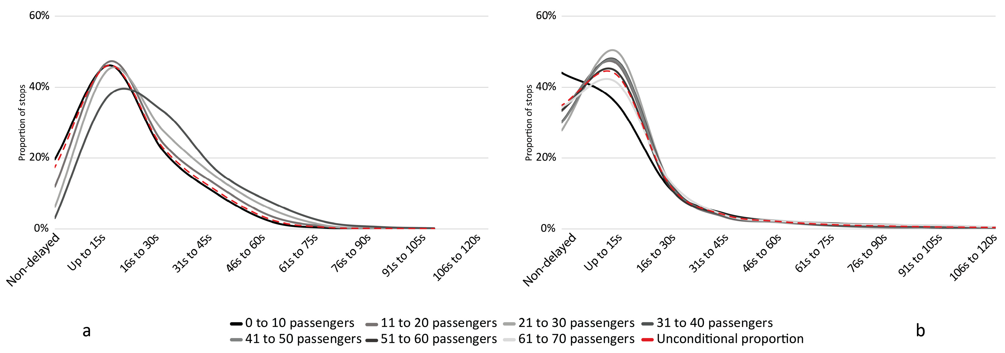
To understand whether the delay frequencies increase or decrease, we plot the proportion of dwell time delays for different passenger volumes for both types of stations under consideration. The results of this are presented in Figure 4. Figure 4a shows the frequency of delays for stations with a scheduled dwell time of 42 s. Two trends can be identified here. When the volume of boarding and alighting passengers exceeds 10 passengers, the frequency of delays starts to increase and differs from the unconditional frequency distribution. The second trend is visible for volumes exceeding 21 boarding and alighting passengers. When this happens, delays larger than 15 s become more frequent. An increase in the volume of boarding and alighting passengers thus leads to an increase in both the frequency and size of dwell time delays at these stations.

A different pattern is visible for stations with a scheduled dwell time of 120 s, as shown in Figure 4b. Stops with 10 or fewer passengers result in a far greater proportion of non-delayed stops compared to the expected proportion of delays and the other groups of passenger volumes. Once passenger volumes start to exceed 10 boarding and alighting passengers, delays of up to 15 s become more prominent. Larger delays, however, follow the expected proportion of delays more closely compared to stops with a scheduled dwell time of 42 s. Although an increase in the volume of boarding and alighting passengers leads to an increase in the frequency of dwell time delays, it does not lead to an increase in the size of delays at stations with a longer scheduled dwell time.

4.4. Pairwise Comparisons

The results of the pairwise comparisons are shown in

Table 3. Pairwise comparison for stations with a scheduled dwell time of 42 s. Significant results are indicated with an *; significance level with Bonferroni correction p < 0.006 (0.05/8 = 0.006).

Passengers	Non-Delayed	Up to 15 s	16–30 s	31–45 s	46 –60 s	61–75 s	76–90 s	91–105 s
0 to 10	0.000 *	0.557	0.000 *	0.000 *	0.000 *	0.000 *	0.000 *	0.010
11 to 20	0.000 *	0.000 *	0.000 *	0.000 *	0.000 *	0.000 *	0.000 *	0.001 *
21 to 30	0.000 *	0.005 *	0.000 *	0.000 *	0.000 *	0.000 *	0.000 *	0.030
31 to 40	0.000 *	0.000 *	0.000 *	0.000 *	0.000 *	0.000 *	0.000 *	0.001 *
41 to 50
51 to 60
61 to 70

and

Table 4. Pairwise comparison for stations with a scheduled dwell time of 120 s. Significant results are indicated with an *; significance level with Bonferroni correction p < 0.006 (0.05/9 = 0.006).

Passengers	Non-Delayed	Up to 15 s	16–30 s	31–45 s	46–60 s	61–75 s	76–90 s	91–105 s	105–120 s
0 to 10	0.000 *	0.000 *	0.006	0.043	0.983	0.122	0.008	0.000 *	0.148
11 to 20	0.057	0.001 *	0.878	0.052	0.408	0.082	0.005 *	0.373	0.454
21 to 30	0.000 *	0.000 *	0.076	0.312	0.288	0.542	0.384	0.883	0.825
31 to 40	0.000 *	0.000 *	0.093	0.250	0.613	0.310	0.811	0.204	0.545
41 to 50	0.000 *	0.000 *	0.857	0.605	0.450	0.065	0.004 *	0.102	0.456
51 to 60	0.138	0.430	0.281	0.503	0.780	0.050	0.060	0.206	0.287
61 to 70	0.689	0.083	0.055	0.986	0.585	0.203	0.048	0.002 *	0.259

for stations with a scheduled dwell time of 42 and 120 s, respectively. All but one of the observed differences are statistically significant for delays of up to 90 s. Although the delay frequencies seem to follow the unconditional distribution when delays become larger than 90 s in Figure 4a, the pairwise comparison shows this is not always the case, as we still find statistically significant differences. Passenger volumes thus also affect the frequency of these larger delays.

For stations with a scheduled dwell time of 120 s, as shown in Table 4, delays of up to 15 s are found to be statistically significantly different from the unconditional frequency distribution up to a total volume of 50 boarding and alighting passengers. Larger delays, however, do not differ significantly from the unconditional frequency distribution, which is in line with the tails in Figure 4b. This further indicates that although the frequency of dwell time delays increases for stations with a scheduled dwell time of 120 s, the delay size is more or less stable across different volumes of boarding and alighting passengers.

4.5. Cohen’s W Effect Sizes

The effect sizes for the observed differences are illustrated in Figure 5. For stations with a scheduled dwell time of 42 s, as shown in Figure 5a, the effect sizes are non-significant across all delay sizes when 10 or fewer boarding and alighting passengers are present. Passenger volumes have a stronger effect on larger dwell time delays, up to delays of 90 s. Differences in the frequencies of such delays can thus be attributed to an increase in the volume of boarding and alighting passengers. Although the pairwise comparisons show that the frequency of delays exceeding 90 s differs significantly from the unconditional frequencies, the effect sizes here are mostly non-significant. Although there is a statistically significant difference, the actual effect of passengers on these larger delays is negligible.

For stations where the scheduled dwell time is 120 s, as shown in Figure 5b, the effect sizes are non-significant for delays greater than 15 s across all volumes of boarding and alighting passengers. There is thus a negligible amount of passengers on delays larger than 15 s. The significant differences found for the pairwise comparison, as shown in Table 4, for the other combinations of passenger volumes and delay sizes thus only have a statistical significance. This further indicates that an increase in the volume of boarding and alighting passengers leads to an increase for the frequency of dwell time delays but not to a substantial increase in the size of these delays.

5. Discussion and Conclusions

The study we present here focuses on the relationship between the volume of passengers and the frequency of different delay sizes. Several previous studies have highlighted that as passenger volumes increase, the passenger exchange time increases as well. Most of those studies indicated a linear relationship where an additional passenger leads to an additional unit of time needed to complete the passenger exchange. However, using multiple years of automatic passenger count data, our analysis shows that although the frequency of dwell time delays increases as passenger volumes increase, the size does not necessarily increase along with it. We also find differences in this trend for the frequencies of delays that are dependent on the scheduled dwell time.

Chi-squared goodness of fit tests revealed statistically significant differences in the frequency distribution of dwell time delay sizes under different volumes of passengers and the unconditional frequency for dwell time delays for both types of stations. Visually analysing the frequencies shows that if passenger volumes are not accounted for, dwell time delays will be routinely underestimated in most cases when passengers are present. Post hoc pairwise comparisons show that the difference between the unconditional and conditional frequencies is statistically significant across the board when dwell times are set at 42 s. Looking at the effect sizes, we find that statistically significant effects exist when passenger volumes start to exceed 10 boarding and alighting passengers. Although pairwise comparisons show statistically significant differences in the tail of the frequency distribution, these effect sizes are found to be negligible. These larger delays are influenced less by the volume of boarding and alighting passengers. When stations have longer scheduled dwell times of 120 s, pairwise comparisons show that significant differences occur only for delays of less than 15 s. The visual graphical analysis shows that when the volume of boarding passengers is low, less than 10 in our case, there are fewer delayed stops. Once passenger volumes start to increase, the frequency of delays starts to increase. The visual analysis also revealed that the frequency distributions start to converge once delays exceed 15 s, which is in line with the results from the pairwise comparisons.

Several things can be mentioned in terms of what this means for dwell times. First, the initial increase in passengers leads to an increase in the frequency of small delays in both types of stations considered. It is, however, not until passenger volumes increase further that the size of the dwell time delays increases as well. Based on our data, this threshold seems to be around 20 boarding and alighting passengers. This value is, however, case specific. For stations that have longer scheduled dwell times, this being 120 s in our case, we only find an increase in the frequency (not size) of smaller delays. Small extensions to dwell time can thus go a long way in terms of reducing the frequencies of delays.

Even at stations with longer scheduled dwell times, delays of 15 s or less are still common, and the frequency of such delays increases with larger passenger volumes. Extending dwell times alone seems insufficient for reducing dwell time delays, as these smaller delays still occur. This leads us to the second observation: speeding up the boarding and alighting process, such as through measures on platforms, can be beneficial for overall punctuality. Although one cannot expect measures aimed at speeding up this process to yield large improvements in boarding and alighting times, our findings here suggest that even small improvements can go a long way.

The findings presented here point in several directions in terms of future studies. Our findings highlight the differences between stations, in our case based on scheduled dwell times with regard to dwell time delay characteristics. Future studies can focus on determining a more detailed metric to characterize stations. An increased understanding in terms of how the type of station influences dwell times can help when faced with the choice as to where we should extend the dwell times. In line with this, our study uses data originating from Stockholm, and it is thus not possible to state whether our findings can be generalized for the entirety of Sweden or in an international context. Future studies should therefore focus on applying a similar method as conducted here to data originating from different geographical areas. Doing so allows for a comparison of the results and a deeper understanding of the effect of context-specific aspects such as the geographical location on the effects that passengers have on dwell times. In terms of data availability, we also see room for future studies. While this study was limited to data aggregated on a train level, future studies could include data on a door-by-door level to ensure that the effects of passengers at different doors, as well as the critical door, can be investigated. Such detailed data provide an important step in further understanding dwell times. Finally, we limit ourselves to the impact of passenger volumes on dwell times, excluding stations with a high likelihood of train interactions and crew changes. This does not mean that such instances are not relevant, however. It can be beneficial to study dwell times at such stations in the future, as this is relevant in understanding dwell time delays in general.

References

- Harris, N.; Graham, D.J.; Anderson, R.J.; Li, H. The Impact of Urban Rail Boarding and Alighting Factors. In Proceedings of the Transportation Research Board 93rd Annual Meeting, Washington, DC, USA, 12–16 January 2014; p. 13. [Google Scholar]
- Vieira, A.P.; Christofoletti, L.M.; Vilela, P.R.S. Analyzing Railway Capacity Using a Planning Tool. In Proceedings of the 2018 Joint Rail Conference, Pittsburgh, PA, USA, 18–20 April 2018; p. V001T04A004. [Google Scholar] [CrossRef]
- Jovanović, P.; Kecman, P.; Bojović, N.; Mandić, D. Optimal allocation of buffer times to increase train schedule robustness. Eur. J. Oper. Res. 2017, 256, 44–54. [Google Scholar] [CrossRef]
- Palmqvist, C.-W. Delays and Timetabling for Passenger Trains. Ph.D. Thesis, Faculty of Engineering, Technology and Society, Transport and Roads, Lund University, Lund, Sweden, 2019. Available online: http://portal.research.lu.se/ws/files/70626078/Carl_William_Palmqvist_web.pdf (accessed on 29 April 2020).
- van Loon, R.; Rietveld, P.; Brons, M. Travel-time reliability impacts on railway passenger demand: A revealed preference analysis. J. Transp. Geogr. 2011, 19, 917–925. [Google Scholar] [CrossRef]
- Brons, M.R.E.; Rietveld, P. Rail Mode, Access Mode and Station Choice: The Impact of Travel Time Unreliability; Research Report for the Project TRANSUMO BTK; VU University: Amsterdam, The Netherlands, 2008. [Google Scholar]
- Bates, J.; Polak, J.; Jones, P.; Cook, A. The valuation of reliability for personal travel. Transp. Res. Part E Logist. Transp. Rev. 2001, 37, 191–229. [Google Scholar] [CrossRef]
- Jiang, S.; Persson, C.; Brundell-Freij, K. Evaluation of travel time reliability using ‘revealed preference’ data & Bayesian posterior analysis. In Proceedings of the 8th International Conference on Railway Operations Modelling and Analysis (ICROMA), Norrköping, Sweden, 17–20 June 2019; p. 10. [Google Scholar]
- Li, D.; Goverde, R.M.P.; Daamen, W.; He, H. Train dwell time distributions at short stop stations. In Proceedings of the 17th International IEEE Conference on Intelligent Transportation Systems (ITSC), Qingdao, China, 8–11 October 2014; pp. 2410–2415. [Google Scholar] [CrossRef]
- Christoforou, Z.; Chandakas, E.; Kaparias, I. Investigating the Impact of Dwell Time on the Reliability of Urban Light Rail Operations. Urban Rail Transit 2020, 6, 116–131. [Google Scholar] [CrossRef]
- Harris, N.G. Train boarding and alighting rates at high passenger loads. J. Adv. Transp. 2005, 40, 249–263. [Google Scholar] [CrossRef]
- Brons, M.; Rietveld, P. Betrouwbaarheid en Klanttevredenheid in de Ov-Keten: Een Statische Analyse; Vrije Universiteit Amsterdam: Amsterdam, The Netherlands, 2007. [Google Scholar]
- Gysin, K. An Investigation of the Influences on Train Dwell Time. Master’s Thesis, Swiss Federal Institute of Technology, ETH, Zurich, Switzerland, 2018. [Google Scholar]
- Seriani, S.; Fernandez, R.; Luangboriboon, N.; Fujiyama, T. Exploring the Effect of Boarding and Alighting Ratio on Passengers’ Behaviour at Metro Stations by Laboratory Experiments. J. Adv. Transp. 2019, 2019, 6530897. [Google Scholar] [CrossRef]
- Goverde, R.M.P. Punctuality of Railway Operations and Timetable Stability Analysis; Netherlands TRAIL Research School: Delft, The Netherlands, 2005. [Google Scholar]
- Kuipers, R.A.; Palmqvist, C.-W.; Olsson, N.O.E.; Hiselius, L.W. The passenger’s influence on dwell times at station platforms: A literature review. Transp. Rev. 2021, 41, 721–741. [Google Scholar] [CrossRef]
- Harris, N.G.; de Simone, F.; Condry, B. A Comprehensive Analysis of Passenger Alighting and Boarding Rates. Urban Rail Transit 2022, 8, 67–98. [Google Scholar] [CrossRef]
- Antognoli, M.A.; Girolami, F.; Ricci, S.; Rizzetto, L. Effect of passengers’ flows on regularity of metro services: Case studies of Rome lines A and B. Int. J. Transp. Dev. Integr. 2018, 2, 1–10. [Google Scholar] [CrossRef]
- Puong, A. Dwell Time Model and Analysis for the MBTA Red Line. Mass. Inst. Technol. Res. Memo. 2000. Available online: http://citeseerx.ist.psu.edu/viewdoc/download?doi=10.1.1.583.7667&rep=rep1&type=pdf (accessed on 28 April 2020).
- Palmqvist, C.W.; Tomii, N.; Ochiai, Y. Explaining dwell time delays with passenger counts for some commuter trains in Stockholm and Tokyo. J. Rail Transp. Plan. Manag. 2020, 14, 100189. [Google Scholar] [CrossRef]
- Buchmueller, S.; Weidmann, U.; Nash, A. Development of a dwell time calculation model for timetable planning. WIT Trans. Built Environ. 2008, 103, 525–534. [Google Scholar] [CrossRef]
- Wiggenraad, P.B.L. Alighting and Boarding Times of Passengers at Dutch Railway Stations; Netherlands TRAIL Research School: Delft, The Netherlands, 2001; pp. 1–21. [Google Scholar]
- Lee, J.; Yoo, S.; Kim, H.; Chung, Y. The spatial and temporal variation in passenger service rate and its impact on train dwell time: A time-series clustering approach using dynamic time warping. Int. J. Sustain. Transp. 2018, 12, 725–736. [Google Scholar] [CrossRef]
- Hansen, I.A. Railway Network Timetabling and Dynamic Traffic Management. Int. J. Civ. Eng. 2010, 8, 14. [Google Scholar]
- Storstockholms Lokaltrafik. Fakta om SL och länet 2016. Stockholm, Sweden, Yearly Report. 2016. Available online: https://www.sll.se/globalassets/2.-kollektivtrafik/fakta-om-sl-och-lanet/sl_och_lanet_2016.pdf (accessed on 28 February 2021).
- Olsson, N.; Halse, A.H.; Hegglund, P.M.; Killi, M.; van der Kooij, R.; Landmark, A.; Seim, A.; Sørensen, A.Ø.; Økland, A.; Østli, V. Punktlighet i Jernbanen—Hvert Sekund Teller; SINTEF Akademisk Forlag: Oslo, Norway, 2015. [Google Scholar]
- MacDonald, P.L.; Gardner, R.C. Type I Error Rate Comparisons of Post Hoc Procedures for I j Chi-Square Tables. Educ. Psychol. Meas. 2000, 60, 735–754. [Google Scholar] [CrossRef]
- Brown, C.G.; McGuire, D.B.; Beck, S.L.; Peterson, D.E.; Mooney, K.H. Visual Graphical Analysis: A Technique to Investigate Symptom Trajectories Over Time. Nurs. Res. 2007, 56, 195–201. [Google Scholar] [CrossRef]
- Keim, D.A.; Mansmann, F.; Schneidewind, J.; Ziegler, H. Challenges in Visual Data Analysis. In Proceedings of the Tenth International Conference on Information Visualisation (IV’06), London, UK, 5–7 July 2006; pp. 9–16. [Google Scholar] [CrossRef]
- Landmark, A.D.; Seim, A.A.; Olsson, N. Visualisation of Train Punctuality—Illustrations and Cases. Transp. Res. Procedia 2017, 27, 1227–1234. [Google Scholar] [CrossRef]
- Wainer, H.; Thissen, D. Graphical Data Analysis. Annu. Rev. Psychol. 1981, 32, 191–241. [Google Scholar] [CrossRef]
- van Oort, N.; Sparing, D.; Brands, T.; Goverde, R.M.P. Data driven improvements in public transport: The Dutch example. Public Transp. 2015, 7, 369–389. [Google Scholar] [CrossRef]
- van Oort, N.; van Nes, R. Line Length versus Operational Reliability: Network Design Dilemma in Urban Public Transportation. Transp. Res. Rec. 2009, 2112, 104–110. [Google Scholar] [CrossRef]
- McDonald, J.H. The Handbook of Biological Statistics. 2014. Available online: http://www.biostathandbook.com/ (accessed on 25 May 2022).
- Lantz, B. The large sample size fallacy. Scand. J. Caring Sci. 2013, 27, 487–492. [Google Scholar] [CrossRef] [PubMed]
- Cohen, J. Statistical Power Analysis for the Behavioral Sciences, 2nd ed.; Erlbaum Associates: Hillsdale, NJ, USA, 1988. [Google Scholar]