Focus on Point: Parallel Multiscale Feature Aggregation for Lane Key Points Detection

Abstract

Lane detection, as a basic environmental perception task, plays a significant role in the safety of automatic driving. Modern lane detection methods have obtained a better performance in most scenarios, but many are unsatisfactory in various scenarios, with a weak appearance (e.g., serious vehicle occlusion, dark shadows, ambiguous markings, etc.), and have issues in simplifying model predictions and flexibly detecting lanes of a non-fixed structure and number. In this work, we abstracted the lane lines as a series of discrete key points and proposed a lane detection method of parallel multi-scale feature aggregation based on key points, FPLane. The main task of FPLane is to focus on the precise location of key points in the global lanes and aggregate the global detection results into the local geometric modeling of lane lines by using the idea of association embedding. Furthermore, this work proposes the parallel Multi-scale Feature Aggregation network (MFANet) in FPLane integrating the context information of multi-scale feature mappings to take full advantage of the prior information of adjacent positions. In addition, MFANet incorporates the Double-headed Attention Feature Fusion Up-sampling module, which can facilitate the network to accurately recognize and detect objects under extreme scale variation. Finally, our method is tested on Tusimple and CULane lane detection datasets; the results show that the proposed method outperforms the current mainstream methods: the accuracy and F1-score of the model are 96.82% and 75.6%, respectively, and the real-time detection efficiency of the model can maintain 28 ms.

1. Introduction

Fully automatic driving mainly includes three core modules: perception, decision making and control [1]. Among them, perception obtains the environmental information around vehicles comprehensively through various sensors and control modules, which is the basis of decision making and control. Lane detection, as a basic environmental perception task, determines the performance of the automatic driving system by its detection speed and accuracy. However, due to the influence of vehicle occlusion, road markings wear, dark–light environment at night and other factors, robustly and quickly detecting lanes is still facing great challenges in practical application.

Traditional lane detection methods highly rely on hand-crafted low-level features, including color, structure tensor, edges and ridge features [2,3,4]. These features are used to obtain lane direction information through Hough transform [5] or Random Sampling Consensus (RANSAC) [6], and then lanes are filtered and fitted out according to the prior information that lanes are parallel to each other and that the distance is fixed. Apart from that, other traditional methods [7,8,9] use mathematical geometric models to describe the geometric structure of lane curves, regarding the lane detection as parameter solutions of the model. Since the hand-crafted features and the strong priori of mathematical models are very sensitive to environmental changes, traditional methods have robustness problems, such as a low detection accuracy and weak generalization ability of models under complex and changeable real-world scenarios.

Deep-learning-based detection methods can achieve pixel-level detection with their powerful representation learning ability and massive data resources. Most lane detection methods [10,11,12,13,14,15] mark lane lines and background pixel points into individual categories by training a convolutional neural network, and predict the position and shape of objects pixel by pixel. The network structure of these methods mainly adopt the high-to-low and low-to-high series codec framework. The high-to-low encoder first generates a low-resolution feature map that includes high-level semantic information; then, the low-to-high decoder is used to recover the feature map to its original resolution, and, finally the pixel-level predictions are output. When the lanes are severely degraded or completely occluded, the series structure, like these methods, often ignores the geometric priori and relevance between lanes themselves, and struggles to extract effective discriminant representations, yielding an inferior detection accuracy.

In addition, some mark the location in the image where each row is most likely to contain part of the lane by a row-wise detection approach [16,17], and others use an anchor-based detection approach to optimize the geometry of the lane curve [18,19,20]. These methods do not focus on the structure of the model but generate a large number of parameterized predictions, which increases the computation costs of the model. Usually, they also require the post-processing (usually a heuristic) to shape parameterized predictions into geometric curves, which further hinders the detection efficiency of the algorithm. To avoid post-processing, the curve parameter prediction strategy is investigated [21,22]. They directly predict parametric equations to express the geometry of lanes, but the limitation is the inflexibility of equations, where only a fixed structure and fixed number of lanes can be detected.

In this work, we abstracted the lane lines with geometric characteristics as a series of discrete key points and proposed a lane detection method of parallel multi-scale feature aggregation based on key points, FPLane. It focuses on the precise location of key points in the global lane line, and the global detection results are aggregated into the local geometric modeling of lane lines by using the idea of association embedding. Moreover, the proposed parallel Multi-scale Feature Aggregation network (MFANet) in FPLane can integrate the context spatial information of multi-scale feature mappings. In addition, MFANet incorporates the newly designed Double-headed Attention Feature Fusion Up-sampling module (DAFU), which is able to facilitate the network to accurately recognize and detect objects under extreme scale variation.

Finally, the main contributions of this paper can be summarized as follows:

• Through abstracting the lane lines as a series of discrete key points, we propose a novel lane detection method based on key points, FPLane. Different from previous detection methods, the proposed method can accurately predict key points of lanes directly from input images or videos, which not only eliminates the need for an object detection box and complicated post-processing, but also reduces the influence of background pixels, thus simplifying the output of the model. Therefore, it is suitable for processing road scenes that include arbitrary numbers or any structures of lanes.
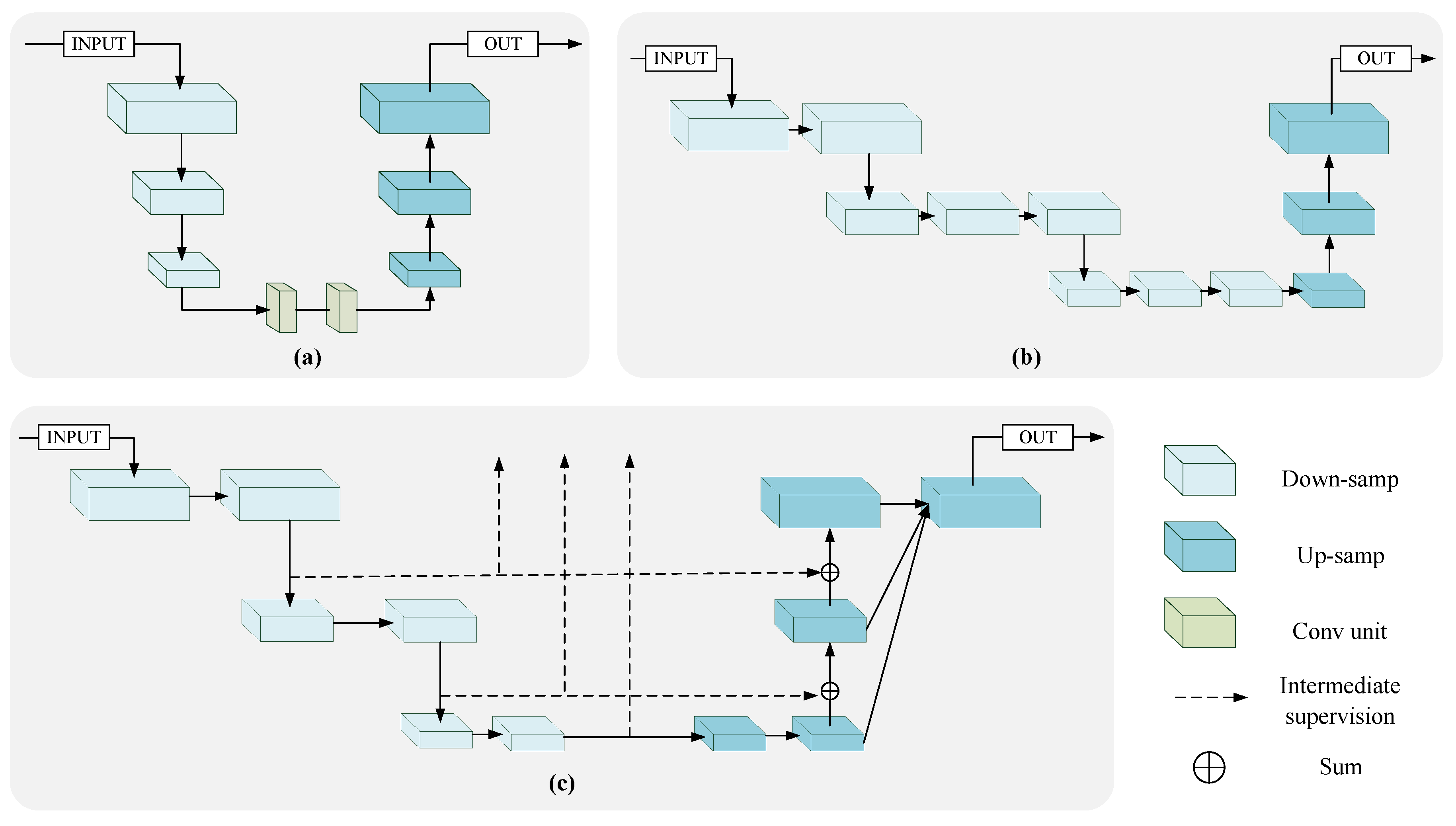
• We propose the parallel Multi-scale Feature Aggregation network to take full advantage of the prior information of adjacent lanes. MFANet can not only extract more discernible representations in complex scenarios with a weak appearance (e.g., vehicle occlusion, road degradation or weak light, etc.), but can also alleviate the information loss in the feature sampling to a certain extent.
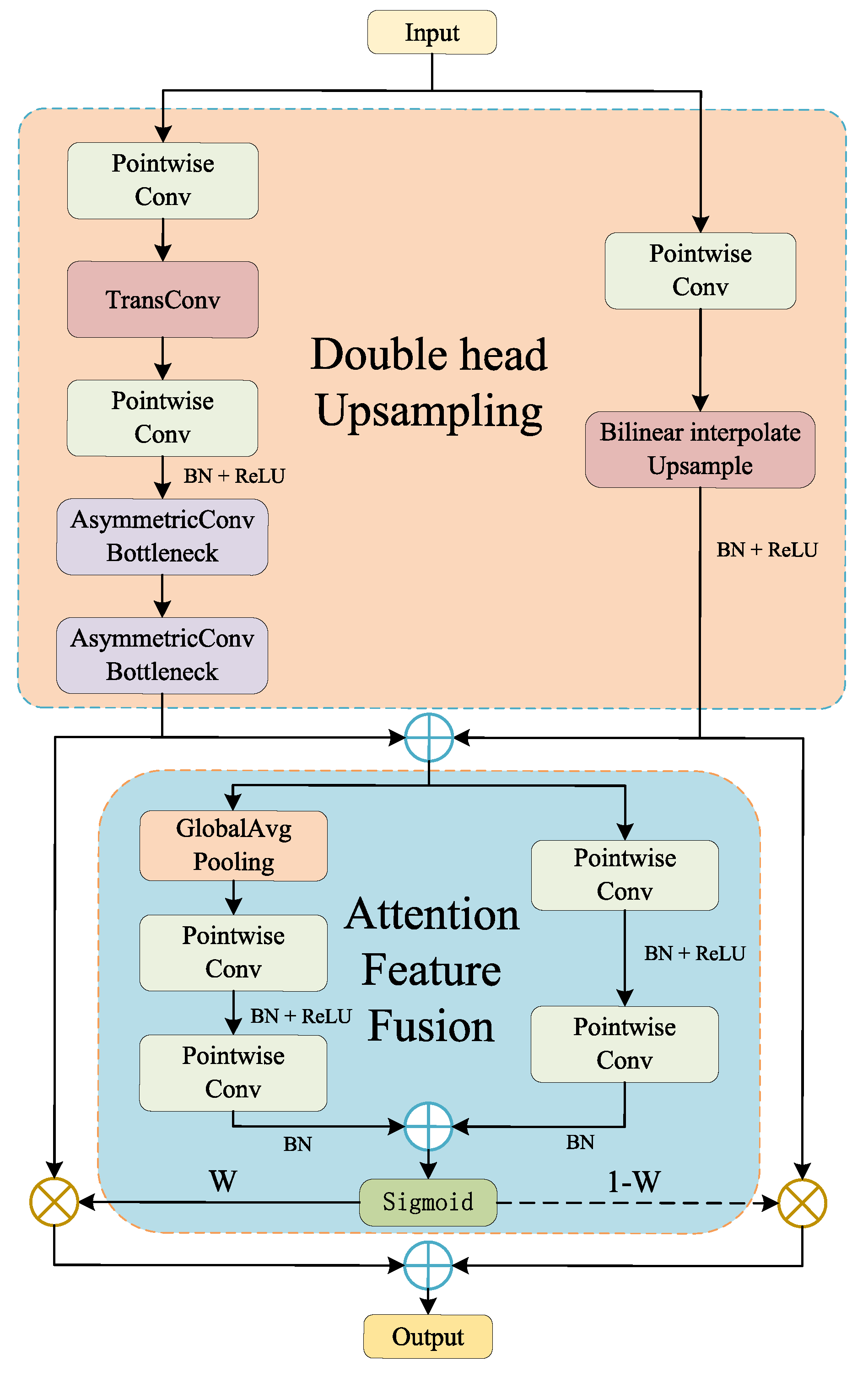
• We propose the Double-headed Attention Feature Fusion Up-sampling module and integrate it into MFANet. This module can precisely cast the sampled feature mapping to the higher resolution representation, and can effectively integrate the spatial information of depth features.

2. Related Work

2.1. Lane Detection

In the field of autonomous driving, lane detection is a significant research topic. In order to meet the requirements of practical application, the detection algorithm must not only have a powerful and fast detection performance, but must also have robustness to adapt to various environments. Refs. [2,3,4,5,6,7,8,9] achieved lane detection through various hand-crafted features and mathematical models, and performed well in simple and clear scenarios. However, when there are extreme road conditions, these algorithms show limitations.

At present, deep learning has become the dominant method in lane detection research. The detection methods based on deep learning can be grouped into two categories: segmentation-based methods and detection-based methods. Segmentation-based methods focus on networks: Ref. [13] proposes a spatial CNN, which passes information between adjacent rows or columns within feature mapping to improve the performance of CNN in detecting long thin shape structures. On the basis of [13], Ref. [11] proposed the recurrent feature-shift aggregator (RESA) to capture the spatial relations of pixels between rows and columns and enrich lane features. Ref. [14] divided lane detection into two stages and proposed a network architecture (LaneNet) that combines semantic segmentation and feature embedding. The network has a shared encoder and two decoders: one of the decoders performs a binary segmentation of lane pixels and background pixels, and the other classifies these lane pixel instances. Ref. [12] proposes a self-attention distillation detection method that forces shallow layers to learn a rich context feature extracted from deep layers, and obtains substantial improvement through self-learning. Ref. [10] predicts the existence and location of lane line markers in the image and groups together instances of lane pixels belonging to the same lane. Ref. [15] proposes a driving scene semantic segmentation method based on embedded loss (EL-GAN), in which, lane markers are segmented based on an input image generator, and segmentation results are judged by a shared weight discriminator.

Detection-based methods focus on outputs of networks. Based on the RPN of faster RCNN, Ref. [19] proposed a line proposal unit (LPU) to predict the horizontal offset of the fixed vertical axis of the proposed line. Ref. [18] proposed a detection model based on anchor points that uniformly sampled pixels of lane along the vertical axis, predicted the offset between sampling points and anchor lines to carry out intensive regression and, finally, applied non-maximum suppression (NMS) to eliminate overlapping predictions and select the lane pixels with the highest score. Ref. [23] defined the lane detection problem from the perspective of multi-key point estimation and association, and used bottom-up local geometric modeling to predict the global structure. Ref. [20] predicted the horizontal axis value of the fixed vertical axis of each lane line, as well as the starting point and end point of the curve, and modeled the shape of lanes based on these predicted values. Ref. [16] predicts a specific feature map and classifies the pixels of each row of the feature map to mark the most likely position of lanes in each row.

2.2. Network Architecture for Key Points Detection

Key points detection is mainly used in human pose estimation [24,25], and the positions of key points can be located by estimating the heatmap. For key points heatmap estimation, the backbone first decreases the input image resolution to facilitate feature extraction and convolution calculation, and then generates a feature heatmap with the same resolution as the input. The main body of the network is possibly augmented with an intermediate supervision and fusion strategy.

Representative network architectures include: (i) a U-shaped mirror symmetric framework. A stacked hourglass network [26] and its subsequent variants [25,27] adopt high-to-low and low-to-high mirror symmetric structures, which transmit information from various scales to deeper depths in order to help the whole model to integrate local and global features and to perform well in detecting centers or edge corners of objects; (ii) an asymmetrical framework with heavy high-to-low and light low-to-high. In [24,28], the high-to-low process is based on a large classification backbone network, such as ResNet or VGGNet, whereas the low-to-high process is simply composed of a few layers of bilinear up-sampling or transpose convolution; (iii) a high-to-low and low-to-high framework with an intermediate supervision or fusion strategy. Ref. [29] proposed a feature aggregation and a coarse-to-fine supervision strategy for multi-stage networks, which improved the results of some existing models to some extent. In the cascaded pyramid network [24], the features generated in the high-to-low process are gradually combined into the low-to-high process through convolutions. Ref. [28] proposed a deep network consisting of several parallel subnetworks, and these subnets conducted a repeated information exchange to eliminate the loss of spatial resolution in the sampling. Figure 1 depicts three representative network architectures mentioned above.

In this paper, we use a set of discrete key points to describe lane lines abstractly, which is similar to the task of human pose estimation. Due to thin and narrow characteristics of lane lines, the backbones with series structures tend to miss subtle details related to lane lines in challenging scenes (such as occlusion, markings wear, dark–light, etc.). To cope with that, this work designed a new network architecture centering on the requirements of this detection task. Although part of the work was inspired by [11,24,25,28,29], there were significant differences overall.

3. Methodology

Based on the above analysis, aiming at the problems of the present mainstream detection methods, such as the struggle to capture effective lane features in complex scenarios with a weak appearance, complicated model predictions and high computation costs, and being limited to fixed structures, this paper proposes a lane detection method of parallel multi-scale feature aggregation based on key points, FPLane. An overview of the method is shown in Figure 2. It takes the lane images obtained by vehicle sensors as the input, and outputs multiple groups of dense key points that represent the final prediction of lane geometry. FPLane mainly consists of three parts: MFANet, global key point detection and grouping key points with association embedding. The functions of each part are as follows.

3.1. Parallel Multi-Scale Feature Aggregation Network

The overall architecture of MFANet is illustrated in Figure 3. The framework consists of an encoder and a decoder, which are connected in parallel. By integrating the context spatial information of multiple-scale feature mappings in parallel, the network can effectively utilize prior information from other lanes to enrich spatial relations about lane lines, which is necessary for cases with conditions such as weak visible lane markings. In addition, MFANet incorporates DAFU, which combines the advantages of interpolation coarse up-sampling and transpose convolution fine up-sampling through the strategy of nonlinear feature fusion. It can cast the sampled feature mapping to the higher resolution representation precisely.

3.1.1. Encoder

The body of the encoder is based on the backbone of HRNet [28] (which was originally designed for human pose estimation), and it consists of four stages of multi-scale parallel subnets. In each stage, repeated multi-scale feature fusion is conducted between parallel subnets. The raw image will be compressed and fused through the encoder to generate abundant multi-scale feature information. As exhibited in Figure 3a, we designed convolution layers of different scales at the end of the backbone network to output these features, and these were progressively integrated into the following parallel decoder.

3.1.2. Decoder

The encoder aims to extract high-level information at a low resolution, whereas the decoder mainly restores the feature mapping to a high resolution through up-sampling. Although the interpolation up-sampling (bilinear interpolation, for instance) method has little information redundancy and a great mapping ability, it is easy to lose image details. Deconvolutional operations and stacking convolutional operations can obtain refined up-sampling results, but it is prone to producing an “uneven overlap” that is similar to a checkerboard pattern artifact. Motivated by the above observations, we advocate the idea of applying the nonlinear feature fusion to aggregate the contextual information from interpolated coarse-sampling and transposed convolution refinement sampling in order to alleviate the problems arising from scale variation in up-sampling. More specifically, we propose the Double-headed Attention Feature Fusion Up-sampling module, as depicted in Figure 4.

Through aggregating contextual information from the different receptive fields along the channel dimension [30], DAFU can precisely cast the down-sampled multi-scale feature mappings to the higher resolution representations and facilitate the network to recognize and detect objects under extreme scale variation. DAFU can be expressed as:

$$\begin{array}{cc}\hfill & D=M\left(T\left(x\right),B\left(x\right)\right)\hfill \\ \hfill & =T\left(x\right)\otimes \delta \left(T\left(x\right)\oplus B\left(x\right)\right)\hfill \\ \hfill & +B\left(x\right)\otimes \left(1-\delta \left(T\left(x\right)\oplus B\left(x\right)\right)\right)\hfill \end{array}$$

(1)

where $T(·)$ is transposed convolution or deconvolution, $B(·)$ is interpolation up-sampling, $M(·,·)$ represents attentional feature fusion, $\delta$ is a sigmoid function and x is the input feature mapping.

As shown Figure 3b, DAFU is the up-sampling module of the decoder, which conducts parallel up-sampling at multiple spatial scales. Assuming that the encoder produces S feature mappings, the decoding process is divided into $S-1$ stages. $X_j^K$ means the j-th feature mapping at the K-th decoding stage. For discussion convenience, we illustrate the first stage decoding as an example. The inputs of the first stage are S feature mappings $\left\{X_1^1,X_2^1,\cdots ,X_s^1\right\}$, and the outputs are feature mappings: $\left\{X_1^1,X_2^1,\cdots ,X_{s-1}^1\right\}$, which are also the inputs of the second stage. The lowest resolution features $X_S^1$ are first sampled by DAFU, and the higher scale feature $M_S^1$ is the output. $M_S^1$ is not only the input of the next stage of decoding, $X_{S-1}^2$, but also combines with the original higher scale feature $F_{S-1}^1$ to form the new fusion feature $X{{}_{S-1}^1}^{\prime }$ through the fusion bottleneck. Then, $X{{}_{S-1}^1}^{\prime }$ is also sampled by DAFU, and the output $M_{S-2}^1$ is both the input of the next stage, $X_{S-2}^2$, and combines with the higher scale feature $X_{S-2}^1$ to form $X{{}_{S-2}^1}^{\prime }$. It will finish until the output $M_1^1$ combines with the feature mapping $X_1^1$ to form $X{{}_1^1}^{\prime }$. The subsequent stages repeat the above steps; the whole procedure can be defined as follow:

$$\begin{array}{cc}\hfill & M_{j-1}^K=D\left(X_j^K,K\right),{}_{j=S-K+1,S-K,\dots ,1;}^{K=1,\dots ,S-1;}\hfill \end{array}$$

(2)

$$\begin{array}{cc}\hfill & X{{}_{j-1}^K}^{\prime }=F\left(X_{j-1}^K,M_{j-1}^K\right),{}_{j=S-K+1,S-K,\dots ,1;}^{K=1,\dots ,S-1;}\hfill \end{array}$$

(3)

$$\begin{array}{cc}\hfill & X_{j-1}^K,X_{j-1}^{K+1}=X{{}_{j-1}^K}^{\prime },M_{j-1}^K,{}_{j=S-K+1,S-K,\dots ,1;}^{K=1,\dots ,S-1;}\hfill \end{array}$$

(4)

In this part, the low-to-high multiscale features generated by the encoder are integrated into the low-to-high decoding process progressively, where the function $D(·,·)$ represents DAFU. The function $F(·,·)$ represents the fusion bottleneck of Figure 3. It is used to combine the feature mapping from adjacent scales with the original scale feature mapping along the channel dimension in the up-sampling process to form the new fusion feature. $M_{j-1}^K$ is the output by the up-sampling of $X_j^K$, and $X{{}_{j-1}^K}^{\prime }$ is the fusion feature generated by $X_{j-1}^K$ and $M_{j-1}^K$.

3.1.3. Analysis of Architecture

In the global perspective, the proposed network is a DCNN (deep convolutional neural network), which takes images or videos as the input, and conjectures lanes accurately by predicting multiple key points sets. The unique design of the framework not only makes full use of the feature extraction capability of the network, but also does not need to repeat the process of high-to-low and low-to-high several times for boosting the performance, which greatly reduces the amount of computation costs and information redundancy. In the local perspective, the network is the parallel connection structure of multiple spatial scales. The multi-scale fusion strategy can help the network integrate spatial information from each scale and enrich global features by other local clues under complex or challenging driving scenarios. In addition, the parallel connection could be regarded as an extended residual connection or skipping connection, which is helpful for coping with the information loss problem in the sampling process of the series structure to a certain extent.

3.2. Global Key Points Detection

For the global key point detection, the network predicts two sets of heatmaps. The first one models the probability space of all target key points, which expresses the probability of existence for each key point. The second predicts the location offset vectors of these key points. Based on them, we are able to locate the exact location of the key points to ensure the geometric accuracy of the final output lane curve. The size of each set of heatmaps is $H\times W$ , but the number of channels is different.

In the training data, each lane curve is annotated as an ordered key points set $l_m=\left\{k_i\right|i=1,2,\cdots ,n\}$, where $l_m$ means the m-th lane curve contains n key points, and $k_i$ is the $i-\mathrm{th}$ point. The network firstly outputs the probability heat map, whose resolution is the same as the input, and the pixel value expresses the probability that the point is predicted as the key point of the lane curve. The key points are considered as the positive sample in the detection task, and each key point of the curve $l_m$ has a ground-truth value, whereas other irrelevant background points are negative samples, as exhibited in Figure 5. As a result of the narrow and long property of lanes, the number of annotated lane points is far fewer than background points. We employed focal loss for the first heatmap, and added the balance factor $\alpha$ on the basis of focal loss to prevent the network bias from a large number of negative samples during training. Furthermore, the farther the pixel cells is from the key points, the faster they converge, which helps the network training to be more concentrated to the pixel cells close to the key points. The following shows the loss function:

$$\begin{array}{cc}\hfill & L_{kp}=\frac{1}{N_k}\left\{{}_{{\displaystyle \sum _{i=1}^{N_k}}\left(1-\alpha \right){\left(p_i\right)}^{\gamma }log\left(1-p_i\right)if{g}_i=0}^{{\displaystyle \sum _{i=1}^{N_k}}\alpha {\left(1-p_i\right)}^{\gamma }log\left(p_i\right)if{g}_i=1}\right.,\hfill \end{array}$$

(5)

where $P_i$ is the probability score of the i-th pixel at the heatmap, $N_k$ is the number of key points in the current image and $g_i$ represents the ground-truth values of positive and negative samples. $\alpha$ is the balance factor, which balances the positive and negative sample loss during training. $\gamma$ is a tunable hyperparameter that controls the penalty for simple samples. The loss function guide the network to learn positive samples and ignores the supervision of background pixels, which makes it easier to process arbitrary numbers of lanes.

In order to gather high-level information and to reduce memory usage, the network maps the raw image to the smaller scale through down-sampling. Pixel locations $\left(x,y\right)$ in the raw image are mapped to the locations $\left(x/\beta ,y/\beta \right)$ in the sampled feature map, where $\beta$ is the scale factor of down-sampling. When the locations are remapped from the feature map to their original resolution, some precision may be lost due to interpolation or deconvolution, which greatly affects the prediction results. Therefore, we used another set of heat maps to predict the location offset vector in order to slightly adjust the locations of key points when they are remapped to the original resolution.

The network predicts the exact location offset vectors for each key point, which includes the horizontal and vertical coordinates. The vectors indicate the correct position of key points, which can make the final prediction result more accurate and smooth. For training, we applied the mean square error (MSE) loss for the horizontal and vertical axis positions:

$$\begin{array}{cc}\hfill & L_{position}=L_{X\_position}+L_{Y\_position}\hfill \\ \hfill & =\frac{1}{N_k}\sum _{i=1}^{N_k}{\left(P_{i\_x}-G_{i\_x}\right)}^2+\frac{1}{N_k}\sum _{i=1}^{N_k}{\left(P_{i\_y}-G_{i\_y}\right)}^2,\hfill \end{array}$$

(6)

Since the background pixels are ignored, only the offset loss of the key points is calculated, where $N_k$ is the number of key points in the current image, $P_{i\_x}$ and $P_{i\_y}$ are the predicted coordinates of horizontal and vertical axes, respectively, and $G_{i\_x}$ and $G_{i\_y}$ are ground-truth values.

3.3. Grouping Key Points with Association Embedding

The global detection results will be aggregated into the local geometric modeling of lane lines in this section. Specifically, we need to further divide the set of detected key points meticulously in order to determine which lane they belong to. To this end, our approach introduced the association embedding idea for human pose estimation in [31]. They generate feature embedding for all detected human joints and group the joints based on the distance between these embeddings. According to this idea, we noticed that, if key points belong to the same lane, the feature distance between their embeddings should be small; on the contrary, the feature distance between embeddings of key points in different lanes should be long. The other branch of the network will generate embedding vectors for each detected key points. We could complete the grouping task only based on the feature distance between embedding vectors of key points, and did not need to pay attention to the actual values of embedding vectors.

In order to group the set of key points belong to the same lane together, $L_{assemble}$ enables the embeddings of these key points to be as close as possible to the cluster center of this lane ${\mu }_l$. For the key points belong to different lanes, $L_{separate}$ is used to separate the cluster centers of different lanes, so that embeddings from different lanes are far away from each other, as shown in Figure 6. The loss function for the embedding is constructed as:

$$\begin{array}{cc}\hfill & {\mu }_l=\frac{1}{K_l}\sum _{i=1}^{K_l}{x}_{l_i},\hfill \\ \hfill & L_{assemble}=\frac{1}{N}\sum _{l=1}^N\sum _{i=1}^{K_l}{∥x_{l_i}-{\mu }_l∥}_2,\hfill \\ \hfill & L_{separate}=\frac{1}{N\left(N-1\right)}\sum _{l_1=1}^N\sum _{\begin{array}{c}{l}_2=1\\ l_2\ne l_1\end{array}}^{N}max\left(0,\mathsf{\Delta }-{∥{\mu }_{l_1}-{\mu }_{l_2}∥}_2\right),\hfill \\ \hfill & L_{GP}=L_{assemble}+L_{separate},\hfill \end{array}$$

(7)

where $x_{l_i}$ represents a key point embedding of lane l, $K_l$ is the total number of key point embeddings of lane l, N is the total number of lanes in the current image, ${\mu }_l$ is the cluster center of the lane l (the mean embedding of the lane l), ${∥·∥}_2$ represents the L2 distance and $\mathsf{\Delta }$ is the distance threshold between cluster centers.

Subsequently, we applied the distance-based embedding clustering method after the model training converged to subdivide the key points of each lane line through the iterative procedure. It specifically includes the following steps:

• Setting the embedding distance threshold ${\delta }_i$ (where ${\delta }_i\le \mathsf{\Delta }$), which is used to determine whether the embeddings belong to the same lane.
• Selecting a random embedding $x_{l_1}$ from all key point embeddings, and assigning a lane label l for it. The value of this embedding $x_{l_1}$ is the initial cluster center ${\mu }_l$ of the lane l.
• Selecting another embedding $x_{l_2}$ from remaining embeddings to calculate the feature distance between $x_{l_1}$ (L2 distance). If the feature distance is less than or equal to ${\delta }_i$, $x_{l_2}$ is assigned to the same label l and the average value of $x_{l_1}$ and $x_{l_2}$ is taken as the new cluster center ${\mu }_l$ of the lane l. Otherwise, proceed to screen the next embedding.
• Repeating step 3 to go through all remaining embeddings and find all embeddings of the lane l.
• A new round of iteration is performed for remaining key point embeddings without labels, and steps 2, 3 and 4 are repeated until all key point embeddings are assigned a lane label.

4. Experiments

In this section, we evaluate the performance of the proposed method FPLane on two common datasets, TuSimple [32] and CULane [13]. Firstly, we introduce the overview of each dataset and the official evaluation criteria, as well as the implementation details of the experiment. This is followed by the results of the comparison with the current mainstream lane detection methods. Finally, the method was discussed and studied through the ablation experiment.

4.1. Dataset

TuSimple and CULane are two popular lane detection benchmarks datasets. TuSimple is relatively simple, and mainly consists of the highway environment with few obstacles, whereas CULane covers various scenarios of the urban road.

Table 1. Basic information of the datasets.

Dataset	Train	Test	Resolution	Road Type	# Lane
Tusimple	3626	2782	1280 × 720	highway	≤5
CULane	88,880	34,680	1640 × 590	urban, rural and highway	≤4

gives the basic information for the two datasets.

(1) TuSimple: TuSimple is one of the large-scale datasets currently used for lane detection tasks. It consists of 3626 training images and 2782 test images. The scenarios are mainly the highway scenarios at different times of the day under good weather conditions. The accuracy is the main evaluation metric of this dataset, and it is defined as the average number of correctly predicted points in the current image. The formula is as follows:

$$\begin{array}{cc}\hfill & accuracy=\sum _{im}\frac{C_{im}}{S_{im}},\hfill \end{array}$$

(8)

where $C_{im}$ denotes the number of correctly predicted points in the current image, and $S_{im}$ denotes the number of ground-truth points in the image. When the difference between the ground-truth point and the predicted point is less than a certain threshold, the point is considered to be correctly predicted. In addition, the false positive (FP) and the false negative (FN) scores are provided:

$$\begin{array}{cc}\hfill & FP=\frac{F_{pred}}{N_{pred}},\hfill \end{array}$$

(9)

$$\begin{array}{cc}\hfill & FN=\frac{M_{pred}}{N_{gt}},\hfill \end{array}$$

(10)

where $F_{pred}$ denotes the number of wrongly predicted lanes, $N_{pred}$ denotes the number of predicted lanes, $M_{pred}$ denotes the number of missed lanes and $N_{gt}$ denotes the number of ground-truth lanes.

(2) CULane: CULane contains 88,880 training images, 9675 validation images and 34,680 test images, covering various scenarios and road types (such as urban and night). At this dataset, the F1-score is the main evaluation metric, and the formula is defined as follows:

$$\begin{array}{cc}\hfill & F1=2\ast \frac{Precision\ast Recall}{Precision+Recall},\hfill \end{array}$$

(11)

where $Precision=\frac{TP}{TP+FP}$ denotes the proportion of the samples with $FP$ in all samples with the predicted value of 1, and $Recall=\frac{TP}{TP+FN}$ denotes the proportion of the samples with $FP$ in all samples with the ground-truth value of 1. $TP$ is the true positive, which means the samples with the predicted value of 1 and the ground-truth value of 1. $FP$ is the false positive, which means the samples with the predicted value of 1 but the true value of 0. $FN$ is the false negative, which means the samples with the predicted value of 0 but the true value of 1.

4.2. Implementation Details

In the experiments, all input images were uniformly resized to 256 × 512 before being fed to the network to reduce computational load, and RGB values of images were normalized to between 0 and 1. For optimization, we used Adam optimizer and poly learning rate decay policy to train model, and the learning rate was set 0.0001 for TuSimple and 0.001 for CULane. The batch size was set to 8, the total number of training epoch was, respectively, set to 500 and 250 for TuSimple and CULane. In addition, we also applied various data augmentation methods, such as Gaussian noise, shadow, translation, random rotation and intensity changing.

The model training and testing were conducted on a computer equipped with the GeForce GTX 1080Ti 12 GB. To save memory and boost computation, most network components were composed of self-written bottleneck blocks in Pytorch. For real-time detection tasks, the average rate of the model can be maintained at approximately 36 frames. The hyperparameters of the above loss functions were determined experimentally, and

Table 2. Parameter settings.

Hyperparameter	Setting
Image size	256 × 512
$\alpha$	0.70
$\gamma$	2
$\mathsf{\Delta }$	1.5
$P{t}_i$	0.81
${\delta }_i$	0.15

shows the setting values of the hyperparameters. $\alpha$ was set to 0.70, $\gamma$ to 2 and $\mathsf{\Delta }$ to 1.5. In the training phase, the confidence threshold of key points $P{t}_i$ was 0.81, and the distance threshold ${\delta }_i$ was 0.15.

4.3. Result

4.3.1. TuSimple

According to the official standard of the TuSimple dataset, the specific evaluation results are shown in

Table 3. Evaluation results on TuSimple dataset.

Algorithm	Accuracy (%)	FP	FN
SCNN [13]	96.53	0.0617	0.0180
LaneNet [14]	96.40	0.0780	0.0244
PointLaneNet [20]	96.34	0.0467	0.0518
LaneATT(ResNet-18) [18]	96.71	0.0356	0.0301
ENet-SAD [12]	96.64	0.0602	0.0205
ERFNet-E2E [17]	96.02	0.0321	0.0428
PINet [10]	96.75	0.0310	0.0250
FPLane (ours)	96.82	0.0315	0.0243

. Due to the limited scale of this dataset and the single scenario (highway), most mainstream methods are close to the saturation accuracy (over 96%). However, without prior training and the use of additional datasets, FPLane still achieved a 96.82% accuracy, a 0.07% improvement over PINet. In addition, it is noteworthy that the FN of FPLane is below other algorithms, which means that our method achieves the lower false detection rate and contributes to a better performance. Figure 7 depicts the visualized test results for the TuSimple dataset.

4.3.2. CULane

As shown in

Table 4. Evaluation results on CULane dataset. F1-score is evaluation metric of the dataset. For crossroad, only FP is shown.

Category	Proportion (%)	SCNN [13]	ENet-SAD [12]	ERFNet-E2E [17]	UFNet [16]	PINet [10]	FPLane (Ours)
Normal	27.7	90.6	90.1	91.0	90.7	90.3	90.6
Crowded	23.4	69.7	68.8	73.1	70.2	72.3	73.4
Night	20.3	66.1	66.0	67.9	66.7	67.7	69.5
No line	11.7	43.4	41.6	46.6	44.4	49.8	48.2
Shadow	2.7	66.9	65.9	74.1	69.3	68.4	74.4
Arrow	2.6	84.1	84.0	85.8	85.7	83.7	86.3
Dazzle light	1.4	58.5	60.2	64.5	59.5	66.3	68.4
Curve	1.2	64.4	65.7	71.9	69.5	65.6	67.2
Crossroad	9.0	1990	1998	2022	2037	1427	1578
Total	-	71.6	70.8	74.0	72.3	74.4	75.2
Runtime(ms)	-	116	51	-	5.7	40	28

, the proposed method achieves a good detection performance on the CULane datasets, with an F1-score of 75.2%. Figure 8 exhibits the visualized test results of the CULane dataset. Compared with some known models, FPLane obtains a superior performance in all scenarios. Compared with PINet (4H), the F1-score of the model improved by 0.8%. Although the proposed method is a detection method based on key points, the performance of the model still has advantages in capturing road representation information of special scenarios, such as road occlusion, incomplete markings, vehicles crowded or weak light.

4.4. Ablation Study

4.4.1. The Effect of Balanced Factor $\alpha$

In this section, the effect of $\alpha$ and different setting values on the performance of the model are explored. In TuSimple and CULane datasets, we tested different settings ($\alpha =0.6,0.65,0.7,0.75,0.8$) and compared them to no settings of $\alpha$. As shown in

Table 5. The testing results of different $\alpha$ settings.

$\mathit{\alpha }$	TuSimple	CULane
	Accuracy (%)	F1-Score (%)
-	96.68	73.8
0.60	96.73	74.4
0.65	96.77	74.8
0.70	96.82	75.2
0.75	96.78	75.1
0.8	96.73	74.9

, the result gets better as the setting value is increased. However, if the setting value is too high, the model may pay too much attention to positive samples, reducing the supervision of negative samples, which make the performance slightly attenuated. Therefore, we finally chose 0.7 as the setting value of $\alpha$.

4.4.2. Effectiveness Analysis of DAFU

This part mainly conducts a quantitative analysis on the effectiveness of DAFU. For comparison, we maintained the basic structure of the model and adopted, respectively, bilinear interpolation up-sampling and transpose convolution up-sampling to carry out 8× up-sampling. In addition, we also analyzed the effects of attention feature fusion (AFF) and direct addition fusion (DAF) in DAFU. The results are shown in

Table 6. Comparison results on CULane dataset.

Upsampling	Fusion Method	F1-Score (%)
Bilinear interpolation	-	72.6
TransConv	-	74.3
DAFU	DAF	74.8
DAFU	AFF	75.2

. DAFU could well improve the lane detection performance, which strongly suggests the effectiveness of the proposed module. In addition, it also shows that the nonlinear fusion method of DAFU is better than the linear fusion method of direct addition.

4.4.3. Parallel Connections in MFANet

We also empirically analyzed the effect of parallel multi-scale connection in network architecture and conducted experiments to study two variants of the network architecture. (1) The parallel connection of the encoder backbone is maintained, but the decoder adopts a direct series connection mode, as shown in Figure 9. Specifically, starting from the lowest scale feature, it is first mapped to the higher scale through DAFU. After that, it is added to the original feature in this scale, and then up-sampled to the higher scale through DAFU again. In this way, each scale feature from the encoder is directly up-sampled layer by layer through DAFU and superimposed together, and the feature with the raw resolution is finally output. In addition, there is no fusion bottleneck in the process. (2) The whole backbone adopts parallel connection, and multi-scale features are fully fused and exchanged in the entire process. This is the strategy we applied. The above networks were both trained from scratch. The results on the CULane testset given in

Table 7. Comparison results on CULane dataset.

Connection Method	F1-Score (%)	Runtime (ms)
Series connection	72.3	25
Parallel connection	75.2	28

show that multi-scale parallel connection is helpful and gains a better performance at the cost of negligible computational efficiency degradation.

5. Conclusions and Future Work

In this paper, we proposed a novel lane detection method of parallel multi-scale feature aggregation based on key points, FPLane. Extensive experiments show that our method obtained a remarkable detection performance and that the proposed modules are effective. The method focuses on the precise location of the key points in the global lanes, ignoring the influence from ambiguous background pixels, which effectively simplifies the output of the model. It can also be applied to various scenes that include arbitrary numbers or any structures of lanes. More importantly, MFANet with the DAFU enables the model capture discriminative information to dope out lanes accurately in complex scenes such as night, shadow and occlusion. The proposed method achieves the state-of-the-art detection performance on Tusimple and CULane datasets: the accuracy and F1-score of the model are 96.82% and 75.6%, respectively, and the real-time detection efficiency can maintain 28 ms.

Since challenging scenarios with a weak appearance do not involve rainy or muddy road conditions in this paper, we plan to build larger datasets with comprehensive challenging situations in the future to enhance the generalization of our proposed method. In addition, another future research direction might be to develop more powerful architectures incorporated into the FPLane framework, such as the ones with the self-attention mechanism or extensible self-supervised learning, to further improve the performance.

References

1. Dun, L.; Guo, Y.; Zhang, S.; Mu, T.; Huang, X. Lane Detection: A Survey with New Results. J. Comput. Sci. Technol. 2020, 35, 493–505. [Google Scholar]
2. López, A.; Serrat, J.; Canero, C.; Lumbreras, F.; Graf, T. Robust lane markings detection and road geometry computation. Int. J. Automot. Technol. 2010, 11, 395–407. [Google Scholar] [CrossRef]
3. Loose, H.; Franke, U.; Stiller, C. Kalman Particle Filter for lane recognition on rural roads. In Proceedings of the IEEE Intelligent Vehicles Symposium, Xi’an, China, 3–5 June 2009; pp. 60–65. [Google Scholar]
4. Chiu, K.Y.; Lin, S.F. Lane detection using color-based segmentation. In Proceedings of the Intelligent Vehicles Symposium, Las Vegas, NV, USA, 6–8 June 2005; pp. 706–711. [Google Scholar]
5. Borkar, A.; Hayes, M.; Smith, M.T. Polar randomized hough transform for lane detection using loose constraints of parallel lines. In Proceedings of the IEEE International Conference on Acoustics, Speech and Signal Processing (ICASSP), Prague, Czech Republic, 22–27 May 2011; pp. 1037–1040. [Google Scholar]
6. Borkar, A.; Hayes, M.; Smith, M.T. Robust lane detection and tracking with ransac and Kalman filter. In Proceedings of the 16th IEEE International Conference on Image Processing (ICIP), Cairo, Egypt, 7–10 November 2009; pp. 3261–3264. [Google Scholar]
7. Xu, S.; Ye, P.; Han, S.; Sun, H.; Jia, Q. Road lane modeling based on RANSAC algorithm and hyperbolic model. In Proceedings of the 3rd International Conference on Systems and Informatics, Shanghai, China, 19–21 November 2016; pp. 97–101. [Google Scholar]
8. Jung, S.; Youn, J.; Sull, S. Efficient Lane Detection Based on Spatiotemporal Images. IEEE Trans. Intell. Transp. Syst. 2016, 17, 289–295. [Google Scholar] [CrossRef]
9. Berriel, R.F.; de Aguiar, E.; de Souza Filho, V.V.; Oliveira-Santos, T. A Particle Filter-Based Lane Marker Tracking Approach Using a Cubic Spline Model. In Proceedings of the 28th SIBGRAPI Conference on Graphics, Patterns and Images, Salvador, Brazil, 26–29 August 2015; pp. 149–156. [Google Scholar]
10. Ko, Y.; Lee, Y.; Azam, S.; Munir, F.; Jeon, M.; Pedrycz, W. Key Points Estimation and Point Instance Segmentation Approach for Lane Detection. IEEE Trans. Intell. Transp. Syst. 2021, 1–10. [Google Scholar] [CrossRef]
11. Zheng, T.; Fang, H.; Zhang, Y.; Tang, W.; Yang, Z.; Liu, H.; Cai, D. Resa: Recurrent feature-shift aggregator for lane detection. arXiv 2020, arXiv:2008.13719. [Google Scholar]
12. Hou, Y.; Ma, Z.; Liu, C.; Loy, C.C. Learning Lightweight Lane Detection CNNs by Self Attention Distillation. In Proceedings of the IEEE/CVF International Conference on Computer Vision (ICCV), Seoul, Korea, 27 October–2 November 2019; pp. 1013–1021. [Google Scholar]
13. Pan, X.; Shi, J.; Luo, P.; Wang, X.; Tang, X. Spatial as deep: Spatial cnn for traffic scene understanding. In Proceedings of the 32th AAAI Conference on Artificial Intelligence, New Orleans, LA, USA, 2–7 February 2018; Volume 32. [Google Scholar]
14. Neven, D.; Brabandere, B.D.; Georgoulis, S.; Proesmans, M.; Gool, L.V. Towards End-to-End Lane Detection: An Instance Segmentation Approach. In Proceedings of the IEEE Intelligent Vehicles Symposium (IV), Changshu, China, 26–30 June 2018; pp. 286–291. [Google Scholar]
15. Ghafoorian, M.; Nugteren, C.; Baka, N.; Booij, O.; Hofmann, M. EL-GAN: Embedding Loss Driven Generative Adversarial Networks for Lane Detection. In Proceedings of the European Conference on Computer Vision Workshops, Munich, Germany, 8–14 September 2018; pp. 256–272. [Google Scholar]
16. Qin, Z.; Wang, H.; Li, X. Ultra Fast Structure-Aware Deep Lane Detection. In Proceedings of the 16th European Conference on Computer Vision (ECCV), Glasgow, UK, 23–28 August 2020; pp. 276–291. [Google Scholar]
17. Yoo, S.; Lee, H.; Myeong, H.; Yun, S.; Park, H.; Cho, J.; Kim, D. End-to-End Lane Marker Detection via Row-wise Classification. In Proceedings of the IEEE/CVF Conference on Computer Vision and Pattern Recognition Workshops, Seattle, WA, USA, 14–19 June 2020; pp. 4335–4343. [Google Scholar]
18. Tabelini, L.; Berriel, R.; Paixão, T.M.; Badue, C.; De Souza, A.F.; Oliveira-Santos, T. Keep your Eyes on the Lane: Real-time Attention-guided Lane Detection. In Proceedings of the 2021 IEEE/CVF Conference on Computer Vision and Pattern Recognition (CVPR), Nashville, TN, USA, 20–25 June 2021; pp. 294–302. [Google Scholar]
19. Li, X.; Li, J.; Hu, X.; Yang, J. Line-CNN: End-to-End Traffic Line Detection with Line Proposal Unit. IEEE Trans. Intell. Transp. Syst. 2020, 21, 248–258. [Google Scholar] [CrossRef]
20. Chen, Z.; Liu, Q.; Lian, C. PointLaneNet: Efficient end-to-end CNNs for Accurate Real-Time Lane Detection. In Proceedings of the IEEE Intelligent Vehicles Symposium (IV), Paris, France, 9–12 June 2019; pp. 2563–2568. [Google Scholar]
21. Tabelini, L.; Berriel, R.; Paixão, T.M.; Badue, C.; De Souza, A.F.; Oliveira-Santos, T. PolyLaneNet: Lane Estimation via Deep Polynomial Regression. In Proceedings of the 25th International Conference on Pattern Recognition (ICPR), Milan, Italy, 10–15 January 2021; pp. 6150–6156. [Google Scholar]
22. Liu, R.; Yuan, Z.; Liu, T.; Xiong, Z. End-to-end Lane Shape Prediction with Transformers. In Proceedings of the IEEE/CVF Winter Conference on Applications of Computer Vision, Waikoloa, HI, USA, 3–8 January 2021; pp. 3694–3702. [Google Scholar]
23. Qu, Z.; Jin, H.; Zhou, Y.; Yang, Z.; Zhan, W. Focus on Local: Detecting Lane Marker from Bottom Up via Key Point. In Proceedings of the 2021 IEEE/CVF Conference on Computer Vision and Pattern Recognition (CVPR), Nashville, TN, USA, 20–25 June 2021; pp. 14117–14125. [Google Scholar]
24. Chen, Y.; Wang, Z.; Peng, Y.; Zhang, Z.; Yu, G.; Sun, J. Cascaded Pyramid Network for Multi-person Pose Estimation. In Proceedings of the IEEE/CVF Conference on Computer Vision and Pattern Recognition, Salt Lake City, UT, USA, 18–23 June 2018; pp. 7103–7112. [Google Scholar]
25. Yang, W.; Li, S.; Ouyang, W.; Li, H.; Wang, X. Learning Feature Pyramids for Human Pose Estimation. In Proceedings of the IEEE International Conference on Computer Vision (ICCV), Venice, Italy, 22–29 October 2017; pp. 1290–1299. [Google Scholar]
26. Newell, A.; Yang, K.; Deng, J. Stacked Hourglass Networks for Human Pose Estimation. In Proceedings of the 14th European Conference on Computer Vision, Amsterdam, The Netherlands, 11–14 October 2016; pp. 483–499. [Google Scholar]
27. Ke, L.; Chang, M.; Qi, H.; Lyu, S. Multi-Scale Structure-Aware Network for Human Pose Estimation. In Proceedings of the European Conference on Computer Vision (ECCV), Munich, Germany, 8–14 September 2018; pp. 713–728. [Google Scholar]
28. Sun, K.; Xiao, B.; Liu, D.; Wang, J. Deep High-Resolution Representation Learning for Human Pose Estimation. In Proceedings of the IEEE/CVF Conference on Computer Vision and Pattern Recognition (CVPR), Long Beach, CA, USA, 15–20 June 2019; pp. 5686–5696. [Google Scholar]
29. Li, W.; Wang, Z.; Yin, B.; Peng, Q.; Du, Y.; Xiao, T.; Yu, G.; Lu, H.; Wei, Y.; Sun, J. Rethinking on Multi-Stage Networks for Human Pose Estimation. arXiv 2019, arXiv:1901.00148. [Google Scholar]
30. Dai, Y.; Gieseke, F.; Oehmcke, S.; Wu, Y.; Barnard, K. Attentional Feature Fusion. In Proceedings of the 2021 IEEE Winter Conference on Applications of Computer Vision (WACV), Waikoloa, HI, USA, 3–8 January 2021; pp. 3559–3568. [Google Scholar]
31. Newell, A.; Deng, J. Pixels to Graphs by Associative Embedding. Adv. Neural Inf. Proc. Syst. 2017, 30, 2172–2181. [Google Scholar]
32. TuSimple. Tusimple Benchmark. Available online: https://github.com/TuSimple/tusimple-benchmark.html (accessed on 6 October 2019).
Figure 1. Illustration of representative networks that rely on the high-to-low and low-to-high series framework. (a) U-shaped mirror symmetric framework. Hourglass [26] and its variants [25]. (b) Asymmetrical framework with heavy high-to-low and light low-to-high. The high-to-low process is based on a large backbone, and the low-to-high process is light [24]. (c) High-to-low and low-to-high framework with intermediate supervision [24] or fusion strategy [28,29].
Applsci 12 05975 g001
Figure 2. Overview of the proposed method. MFANet incorporates DAFU and generates two sets of prediction from the input images. Subsequently, the key points of global lane line can be accurately conjectured base on these resulting prediction sets. Finally, association embedding strategy is utilized to make the final local geometry of lane curves.
Applsci 12 05975 g002
Figure 3. Overall architecture of MFANet. It is composed of encoder and decoder. Encoder adopts the backbone of HRNet [27] for more efficient multi-scale feature extraction. It consists of four stages of multi-scale parallel subnets. Decoder consists of DAFU, which recovers multi-scale features to the original size precisely.
Applsci 12 05975 g003
Figure 4. Double-headed Attention Feature Fusion Up-sampling module. DAFU combines the advantages of interpolation coarse up-sampling and transpose convolution fine up-sampling through attention feature fusion method, and recovers the down-sampled feature map to 2× size.
Applsci 12 05975 g004
Figure 5. Illustration of key points prediction. ‘Green’ grids are background pixels, and the grids marked ‘blue’ are key points of the lane curve.
Applsci 12 05975 g005
Figure 6. Associatiom embedding of key points. L a s s e m b l e enables the embeddings of these key points as close as possible to the cluster center of this lane μ l . L s e p a r a t e is used to separate the cluster centers of different lanes.
Applsci 12 05975 g006
Figure 7. Visualized results of FPLane on TuSimple testing set. The second row is labels and the third row is predicted results of FPLane.
Applsci 12 05975 g007
Figure 8. Visualized results of FPLane on CULane testing set. The second row is labels and the third row is predicted results of FPLane.
Applsci 12 05975 g008
Figure 9. The decoder with the series connection.
Applsci 12 05975 g009