
On Hyperbolic Complex Numbers


Institute of Mathematics, University of Rostock, 18051 Rostock, Germany
Appl. Sci. 2022, 12(12), 5844; https://doi.org/10.3390/app12125844
Submission received: 13 May 2022
/
Revised: 2 June 2022
/
Accepted: 4 June 2022
/
Published: 8 June 2022
(This article belongs to the Special Issue Real, Complex and Hypercomplex Number Systems in Data Processing and Representation)
Abstract
:For dimensions two, three and four, we derive hyperbolic complex algebraic structures on the basis of suitably defined vector products and powers which allow in a standard way a series definitions of the hyperbolic vector exponential function. In doing so, we both modify arrow multiplication, which, according to Feynman, is fundamental for quantum electrodynamics, and we give a geometric explanation of why in a certain situation it is natural to define random vector products. Through the interplay of vector algebra, geometry and complex analysis, we extend a systematic approach previously developed for various other complex algebraic structures to the field of hyperbolic complex numbers. We discuss a quadratic vector equation and the property of hyperbolically holomorphic functions of satisfying hyperbolically modified Cauchy–Riemann differential equations and also give a proof of an Euler type formula based on series expansion.
1. Introduction
QED. These three letters are often found at the end of a mathematical proof or even an entire mathematical paper, but what meaning can they have at the beginning of a work, this work? It is the great historical importance that quantum electrodynamics has for the application of complex numbers and vector multiplication outside mathematics. In [1], this connection is presented in a very impressive way for a broad readership. Arrow combination and in particular multiplication form the technical basis there for the mathematical treatment of physical phenomena such as reflection and diffraction and many others. The interactive computer animation programs in [2] make it possible to simulate such physical phenomena on the computer in a fascinating way. The reader is invited to create similar animation programs based on the present mathematical results. For an application of vector multiplication when using photo manipulation programs, we refer to [3].
If complex numbers are not adequate to describe certain mechanical [4], or other physical [5,6,7] or technical [8] processes then their generalizations or modifications may be of interest. Hyperbolic complex numbers which are usually represented as
are strictly related to space-time geometry of two dimensional special relativity [9,10,11]. Here, is understood as an abstract or independent quantity taken from somewhere else outside of Hyperbolic complex numbers were developed in [10,12,13,14,15] and are also known by several other names, such as, e.g., perplex numbers [9], split complex numbers [5,9,16,17], space-time numbers [18], dual numbers [6], double numbers [8,10] as well as twocomplex numbers [19], to name just a selection of the numerous possible references.
In this context, the hyperbolic exponential function is defined in [9,15,20] for by
where and the hyperbolic rotation of an angle transforms a vector in the new vector
The quantity is invariant with respect to hyperbolic rotation.
The generalized complex multiplication discussed in [11] includes the ordinary product
the Study product
and the Clifford product
as particular cases. A somewhat different approach to hyperbolic complex numbers is provided in [21] by the use of so called jay-vectors,
Does it make things easier to answer the questions of the existence and possible uniqueness of the abstract or formal quantities and operations encountered when having two non-identical approaches, (1) and (4), to the hyperbolic complex unit? How about the true character of this unit? Mathematical quantities are usually defined by positively stating their properties instead of excluding certain properties, as is the case with “”.
Some new aspects concerning existence and (non-)uniqueness of usual complex numbers as realizations of a general algebraic structure are derived in [22,23,24,25]. There is only briefly mentioned here a property that stands in a certain connection with [1]. There certain probabilities are calculated as length squares of sums of two vectors. If parallel vectors of length 0.2 are oriented in the same direction or in opposite directions, the results are 0.16 and zero, respectively. However, if two such vectors are perpendicular to each other, the value 0.08 results according to the Pythagorean theorem. In [1], reference was made to the fascinating fact that these probabilities are experimentally verified with extremely high accuracy. If one is only interested in obtaining the above three results, any of the vector multiplications from [22] can be used, which might be of some interest for further considerations of physical or other phenomena.
In the present paper, we follow as closely as possible the way taken in [22,23,24,25]. As a result, it becomes possible to generalize hyperbolic complex numbers into different directions. Here, we present multivariate generalizations. We further develop the historically close connection between complex analysis and vector algebra by defining a hyperbolic exponential function using a suitable definition of vector product and power for the definition of the exponential function through a series expansion. While in [22] a vector product based on the ordinary product was introduced, here, to correspondent to Definition 6 of a geometrical hyperbolic vector product, we will introduce a vector product based on the Clifford product.
The paper is organized as follows. We start in Section 2.1, Section 2.2 and Section 2.3 by introducing a hyperbolic vector product, which allows the subsequent introduction of hyperbolic vector powers and a hyperbolic vector exponential function. The latter, as well as the hyperbolic rotation, will therefore be introduced differently than in (2) and (3). In Section 2.4 and Section 2.5, we discuss a quadratic vector equation and modified Cauchy–Riemann differential equations. The slightly modified hyperbolic complex algebraic structure considered in Section 2.6 is based upon a vector product that is a geometrically motivated modification of the vector product being related to the Clifford product. In Section 3, we treat space-time or spherical-hyperbolic complex numbers in dimensions three and four. We close with a discussion in Section 4 and Appendices Appendix A and Appendix B.
We leave it to the reader to choose other basis elements of the underlying event spaces than those chosen here. In [23], it was discussed in detail that changing the basis elements of an event space does not affect the basic properties of the complex algebraic structures considered there. This also applies here.
2. The Basic Hyperbolic Complex Algebraic Structure
2.1. Vector Algebra
Let
denote an event space, that is the set of possible outcomes of an experiment or the light cone in the physical interpretation or just a set of possible observations of interest on which multiplication with positive real numbers is defined to be the function where .
Definition 1.
The vector addition is defined componentwise as
If there exists such that , then we say that can be subtracted from or is additively reachable from or event influences event . In this case, we write
and call the operation the operation of constrained vector subtraction.
Let
and assume that vector addition and constrained vector subtraction are defined analogously on
Definition 2.
The analytical hyperbolic vector product of and is defined as
where
The k’th hyperbolic vector power of and the hyperbolic vector exponential of z are defined by
and
respectively.
We emphasize that we exclusively use the product for defining the hyperbolic exponential of z. For our motivation for doing so, we refer to Remark 2 below. Vector product and exponential can also be understood as arrow product and exponential in the sense of [1].
Definition 3.
The analytical hyperbolic vector product of and is defined to be a random variable on an abstract probability space that takes the values and accordingly with probabilities and .
Notice that
If you look at Definitions 2 and 3 together, the hyperbolic vector product is a function
Because the focus of our consideration is , we do not consider on combinations of and .
Example 1.
The vector is the additive neutral element. Let If then
That is, within is the multiplicative neutral element. On the other hand, if then
Here is the result of reflecting the point at the line
Definition 4.
If for and from there exists such that , then we say that can be divided by and call the operation the operation of constrained vector division. If can be divided by , then we call the inverse of z.
Notice that if has an inverse, then
The vector product is obviously commutative and the second up to the fourth hyperbolic vector powers of are
and
respectively.
2.2. Geometry
If and , then . The Lie group on is thus generated by the multiplications with the elements from the unit half-circle In other words, if the function is defined by , then multiplication of by any leaves invariant.
Definition 5.
The hyperbolic coordinate transformation , , is accordingly defined as
Here, the notation indicates whether the signed area content ψ is measured counterclockwise between and or clockwise between and see Figure 2.
The union of all -sectors represents a disjoint decomposition of the cone , see Figure 2.
The transformation therefore has an a.e. uniquely determined inverse , which is given by with
Remark 1.
With the quantity equals two times the signed area content of the hyperbolic sector the boundary of which is marked with the help of the points and see Figure 3.
For an elementary geometric proof of this remark, we refer to Appendix A.
Definition 6.
The geometrical hyperbolic vector product of and being both either from or from is defined as
The expression on the right side of the last equation is always uniquely defined because due to Remark 1 the sum represents the finite content of a bounded hyperbolic sector (triangle), which itself is a subset of an unbounded set having infinite area content, see Figure 4.
Let and let
denote a hyperbolic sector (or hyperbolic triangle) spanned by the points see Figure 5. Additionally, let be a transformation defined by
Then,
Theorem 1.
The transformation is area-preserving.
Proof.
We show that does not change the content of a hyperbolic sector. The area content of such sector is
□
If and , then the geometrical hyperbolic vector multiplication may be reflected by sector combinations of two types. Since there is no a priori preferred variant for one of two possibilities of assigning the sum of signed area contents, they can be regarded as occurring randomly. The following definition may thus be considered being well motivated.
Definition 7.
The geometrical hyperbolic vector product of and is defined to be a random variable on an abstract probability space, which takes the values and accordingly with probabilities and .
Theorem 2.
The geometrical and analytical hyperbolic vector products are equal.
Proof.
If then by (8),
It follows from this and the definitions of the hyperbolic functions that
If or and then the proof follows analogously. □
2.3. Complex Analysis
A classical way to introduce complex numbers is to say that they allow the representation where x and y are real numbers and is a formal quantity coming from somewhere other than and satisfying . The reader of such a definition is then tacitly asked to believe that the quantity exists in the sense that it can be assigned a strict mathematical meaning and that the operation of squaring this “imaginary unit” agrees or harmonizes with the operation usual in the realm of real numbers. The reader is also left alone with thinking about the possible uniqueness of such a quantity. The answer to this challenge can vary. One can try to take for a vector or a matrix and in each case define a corresponding multiplication rule. However, the usual squaring of vectors and matrixes does not result in the number −1. Therefore people in usual complex number theory sometimes say that they “identify” the vector with the real number , without saying, however, what an “identification” is other than an equation. However, obviously does not equal −1. In [26], it is alternatively discussed that a complex number has a dual real value nature, i.e., is capable of two values without being able, however, to fully explain it. We recall that Definition 3 of the present work gives a well motivated explicit definition of a two-valued random hyperbolic vector product.
In [22,23,24,25], algebraic structures are introduced, within which the “imaginary unit” is always explicitly given as a well-defined element from the vector space underlying this structure. Here, we follow this approach as closely as possible and therefore necessarily extend the event space. Just as the imaginary unit does not belong to the real line if one describes complex solutions of quadratic equations over see Section 2.4 and [24], the vector
obviously does not belong to the originally considered event space but belongs to the set . Note that
and
Remark 2.
If one follows usual hyperbolic number notation and writes
instead of (9), then one is tacitly using the multiplication rule, which is well motivated for elements of for the element of . This motivates our definition of the hyperbolic exponential in Definition 2.
The hyperbolic vector exponential of allows a representation that is reminiscent of Euler’s well-known trigonometric representation of usual complex numbers, where, however, the so called imaginary unit is replaced with vector and the trigonometric functions sine and cosine are replaced with hyperbolic functions.
Theorem 3.
The following hyperbolic Euler-type formula holds true:
Proof.
The rearrangement of the infinite vector sum
is allowed due to its convergence properties. Finally, the definitions of the hyperbolic functions apply. □
Note that belongs to the observation set , but comes from a well-defined other set and the hyperbolic vector multiplication rule is explained in the extended event space. In contrast to the classical approach to complex numbers, however, is explicitly known, here. The following definition is now well motivated.
Definition 8.
We call a hyperbolic complex algebraic structure with and being the additive and multiplicative neutral elements and the hyperbolic element satisfying (9).
We recall from [23] that changing the basis elements of an event space may be very useful and does not affect the basic properties of the complex algebraic structure.
2.4. Solving a Quadratic Vector Equation
If , then the quadratic equation
has the real solutions . The structure of these solutions reproduces if one considers the quadratic vector equation or
The result
is graphically illustrated in Figure 6. For a closely related geometric discussion of quadratic vector equations with respect to -vector multiplication, we refer to [24].
2.5. Hyperbolically Modified Cauchy-Riemann Differential Equations
Let According to Definition 4, we call hyperbolic multiplicative reachable from if there exists such that . If this is so, then we call the hyperbolic ratio of and and write this as
One can check that
and in particular
If we apply (13) also for and , then
While means the identity mapping, the mapping means reflection of the point at the line .
Let D be an open subset of . A function is called hyperbolically differentiable in if the ratio converges to a limit point , say, as , that is
The function f will be called hyperbolically holomorphic in D if it is differentiable in every from D. If such function is given by
then it follows that hyperbolic modifications of the well known Cauchy–Riemann differential equations hold. To become more specific, we consider points with
Letting now the values of h tending to zero, and, respectively, denoting the partial derivatives with respect to x or y of a function by and , we get
where is a certain number from the interval . Similarly,
The following theorem has thus been proved.
Theorem 4.
The hyperbolically holomorphic function , satisfies the hyperbolically modified Cauchy–Riemann partial differential equations
Consequently, hyperbolically holomorphic functions have the property
2.6. A Slightly Modified Hyperbolic Complex Algebraic Structure
Let us assume that the definition of the hyperbolic coordinate transformation is changed so that now the signed area content is measured counterclockwise between and , see Figure 7. Then, slightly different from Definition 5, it follows that
For the geometric definition of the hyperbolic vector product, it then results that, in ,
Overall, the analytical and geometric definitions of the hyperbolic vector product are then
and in ,
The result is a modified hyperbolic complex algebraic structure where if and still then
and if then
Here, is the result of rotating counterclockwise by .
3. Spherical Hyperbolic Complex Numbers
3.1. Three Dimensional Space-Time Structure
Let now
be a hyperbolic half-sphere of hyperbolic radius and assume that the event space is the cone
We recall that a class of new analytical vector products in is introduced in [23]. Here, we consider a hyperbolic analog as follows.
Let Unless for for at least one value of the analytical hyperbolic vector product of and is defined as
Moreover, we put
It should be noted that this product differs only slightly from (12) and (13) in [23]. To better understand this vector product, we first introduce a new coordinate system.
Definition 9.
With the notation we define the hyperbolic coordinate transformation by
With , the a.e. uniquely defined inverse map is given by
The event space is a subset of the vector space . The latter has the set of vectors and as a basis. The subspaces spanned by or are, respectively, denoted by and and the orthogonal projections of the vector onto the spaces by and , respectively. It is recalled that in [23], it was discussed what technical implications the choice of a different basis of the vector space or the choice of another three-dimensional space may have. Such a choice obviously depends on the specific application at hand and also applies to the hyperbolic model.
The variable describes the angle between the vectors and , which one can imagine in Figure 8.
If the angle runs through the interval , then the point runs through an Euclidean circle of radius , centered at the point and belonging to the two-dimensional plane being parallel to the subspace
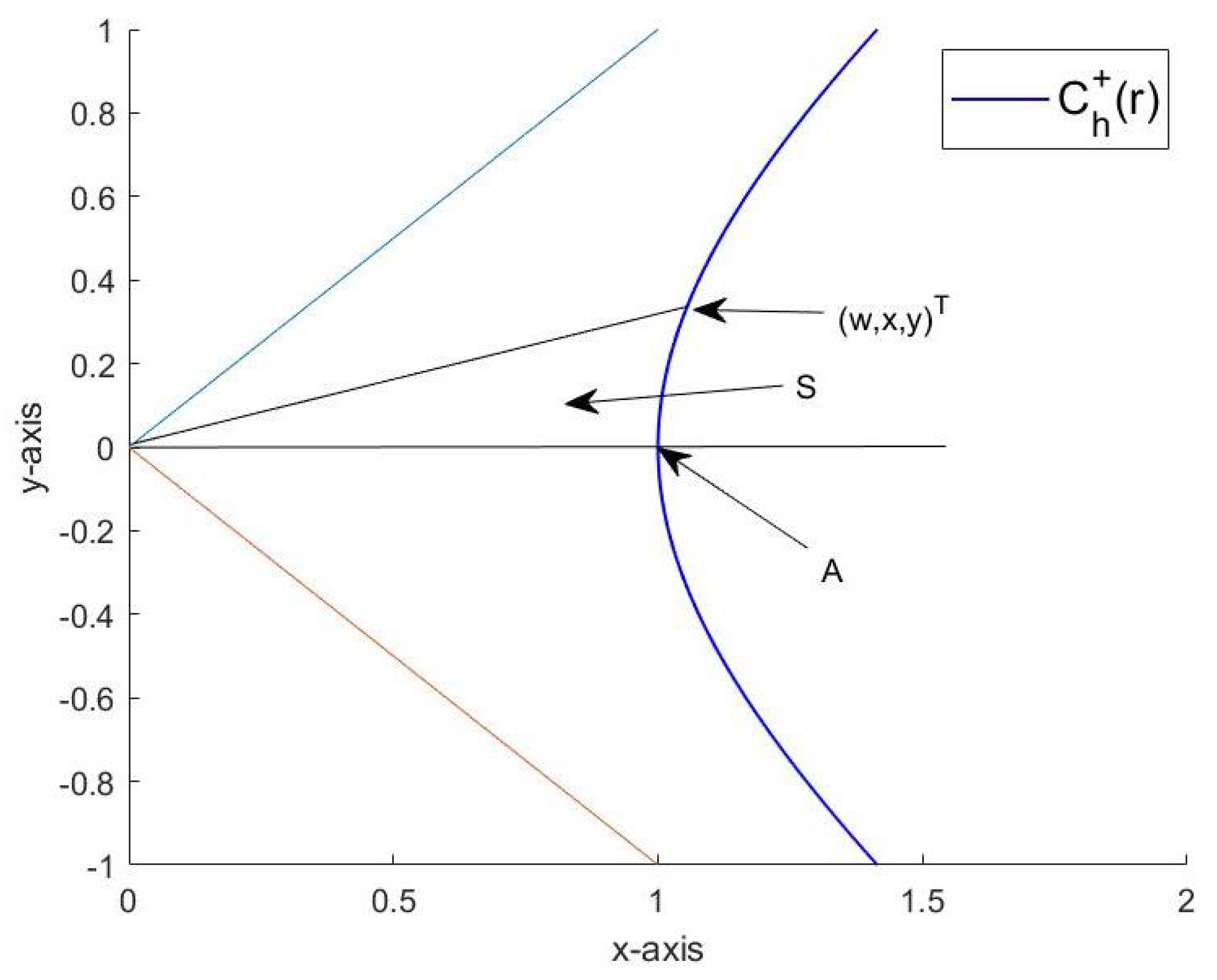
If the intersection point of and is denoted A and denotes the hyperbolic sector built by the points and A then equals the area content of S, see Figure 9.
The meaning of r and lacking as a hyperbolic radius and an angle, and as a non-negative area content motivates the following geometric definition of a vector product in .
Definition 10.
The geometric hyperbolic vector product of and is defined as
where
Theorem 5.
The geometric hyperbolic vector product of and equals the analytical hyperbolic one.
Proof.
The proof of this theorem follows the line described in Section 2. □
Example 2.
It is supposed to, respectively, mean ⊕ and • vector addition and scalar multiplication in the usual sense.
3.2. Four Dimensional Space-Time Structure
Let now a hyperbolic half-sphere of hyperbolic radius be defined as
and the event space or space-time cone as
We recall that a class of new analytical vector products in is introduced in [25]. Here, we consider a hyperbolic analog as follows.
Definition 12.
Let
Unless for or for at least one value of the analytical hyperbolic vector product of and is defined as
Moreover, we put
and
where .
It should be noted that Formula (16) differs only slightly from Formula (12) in [25], namely with respect to two times the factor . One of these factors is due to the circumstance that is a one-sided cone and the other factor is caused by the fact that instead of a norm used in [25] we use an antinorm according to [27], here. To better understand this vector product, we first introduce a new coordinate system.
Definition 13.
With the notation we define the hyperbolic coordinate transformation by
With , the a.e. uniquely defined inverse map is given by
The event space is a subset of the vector space . A basis of the latter consists of the vectors and . The subspaces spanned by or are, respectively, denoted by and and the orthogonal projections of the vector onto the spaces by and , respectively.
The meaning of r and lacking as a hyperbolic radius and two angles, and as an area content motivates us for the following definition.
Definition 14.
We define the geometric hyperbolic product of the vectors and as
where
Theorem 6.
The analytical hyperbolic vector product of and equals the geometric hyperbolic one.
Proof.
The proof of this theorem follows the line described in Section 2. □
Example 3.
It is supposed to, respectively, mean ⊕ and • vector addition and scalar multiplication in the usual sense.
Definition 15.
We recall once again from [23] that changing the basis elements of an event space can be very useful and does not affect the basic properties of the complex algebraic structure under consideration.
4. Discussion
Why do we allow applying the rule in (5) to the extended event space when it is originally defined only for pairs of elements of either or ? To approach an answer, let us first recall the situation with usual complex numbers as described at the beginning of Section 2.3. Since there is certainly no explanation for as a “number”, there is no explanation for in this approach.
However, for centuries, successful applications of complex numbers have provided the motivation to deal with them, even though there is a certain lack of mathematical rigor in their definition. Practical success in using imaginary numbers was taken as proof of their existence, which is rather untypical for pure mathematics. The strict approaches in [22,23,24,25] have overcome this deficit for the usual complex numbers and their certain generalizations by giving explicit vectorial definitions of the imaginary unit.
The meaning of complex numbers has evolved over a historically lengthy process. While complex numbers initially played a formal role in solving quadratic equations, they later became an indispensable tool in many applied sciences, e.g., in electrical engineering where the current I and voltage U in an alternating current circuit satisfy the equation in time t. In the event that other quantities and satisfy the equation , p-generalized complex numbers were introduced in [22]. Higher dimensional and other generalizations were considered in [23,24,25].
In two-dimensional space-time models, quantities X and T that satisfy the equation are of interest. In such a case, ordinary complex numbers do not provide an adequate description, but hyperbolic complex numbers. Such numbers, together with their multidimensional generalizations, have been introduced in the present work. This could pave the way for numerous potential applications of generalized complex analysis. Just as the existence of a verifiable usual imaginary unit was unclear for a long time, so was for the hyperbolic imaginary unit. This gap was closed in the present work and concrete vector representations for the hyperbolic imaginary unit were given. Since the properties of each vector are essentially determined by the properties of the space containing it, the choice of a vector space is of great importance when processing a specific application. In particular, it is of great importance to empirically verify the validity of a vector multiplication or arrow combination in the respective application and to develop corresponding computer animation programs as was mentioned in the Introduction for the QED. A hopefully broad readership from different application areas is invited to follow this path. The creation of interactive computer animation programs in the sense of [2] but for vector multiplication as in the present work can be a building block of such a project.
Funding
This research received no external funding.
Conflicts of Interest
The author declares no conflict of interest.
Appendix A. Proof of Remark 1
For completeness, we give here an elementary proof of the well known result stated in Remark 1. It follows from (24) and the definitions of the hyperbolic functions that This proves the first statement in (8). The matrix
describes an orthogonal counterclockwise rotation by angle around the origin of . Let
and
see Figure A1.
Figure A1.
.
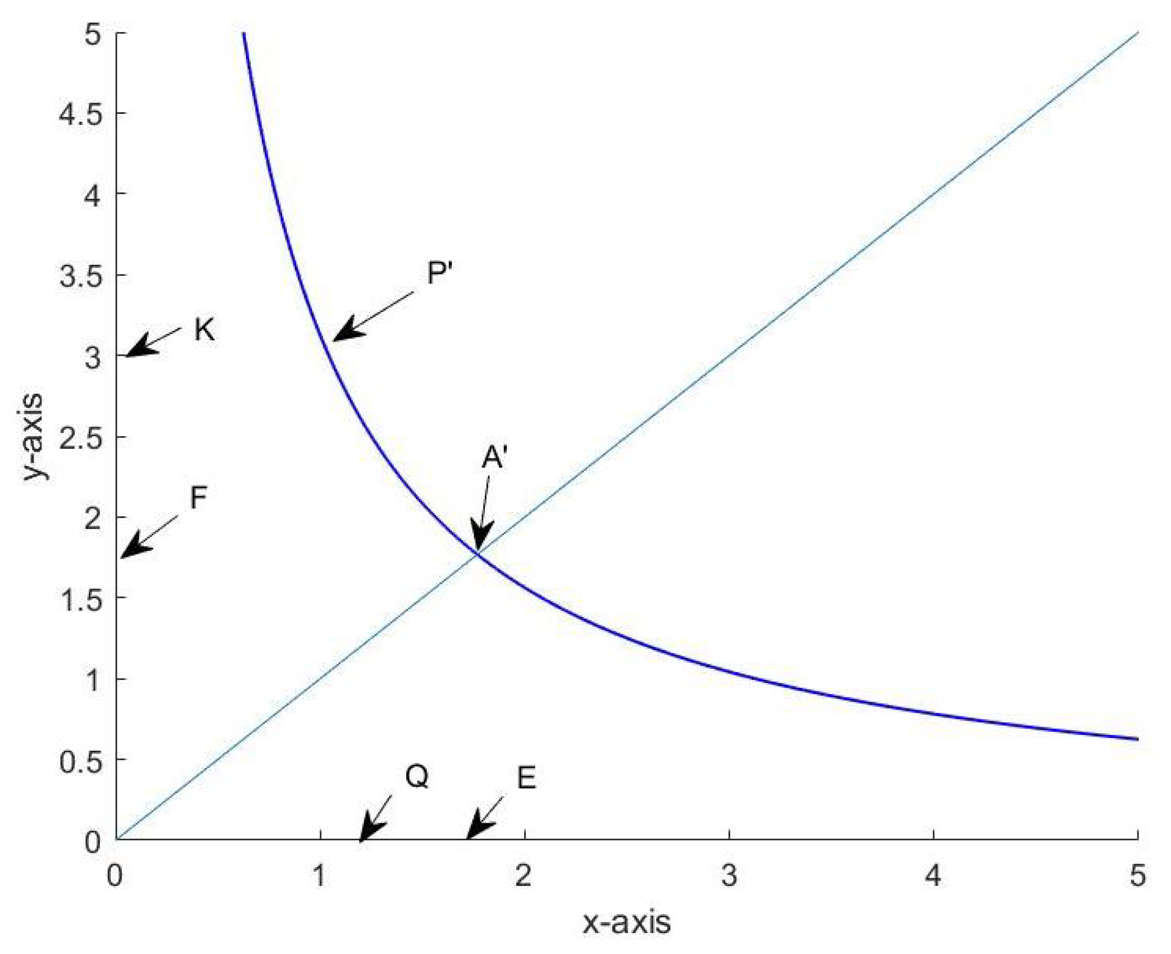
We denote the projection points of and on the -axis with Q and E and accordingly those on the -axis with K and F. The distances from these points to the point are denoted and , respectively. Let . Then,
The area contents of the triangles and are
The hyperbolic trapezoids and allow the disjoint decompositions
such that
It follows from (A1) and (A2) that the area contents of the hyperbolic sector and the hyperbolic trapeze satisfy
Notice that
It follows from (A4) and (A5) that
with
One can show in an analogous way that
also holds. It follows from the latter equation and (A7) that
and
This proves the second equation in (8), thus Remark 1 is true with
Appendix B. Is a Semi-Antinormed Space
In this section, we give an elementary proof of the statement presented in the first part of Example 5.2 in [27] from which it follows that if denotes the indefinite quadratic form defined by then is a semi-antinormed space. To this end, we prove that a certain distance function defined on the hyperbolic circle satisfies a reverse triangle inequality.
Definition A1.
If the point is additively reachable from the point , then is called their hyperbolic distance.
Theorem A1.
If then
Proof.
If , then
Thus,
□
This theorem means that the hyperbolic distance function satisfies the reverse triangle inequality. We refer to [27] for more details.
References
- Feynman, R. QED: The Strange Theory of Light and Matter; Princeton University Press: Princeton, NJ, USA, 1985. [Google Scholar]
- Szántó, L. Neobycejná Teorie Svetla a Látky. Animace Feynmanovych Obrázku Svetla Podle QED. Aktualizováno. 2011. Available online: https://www.kosmas.cz/knihy/195930/neobycejna-teorie-svetla-a-latky (accessed on 8 April 2022).
- Aspden, J.L. 2013. Available online: www.learningclojure.com/2013/10/feynmans-arrows-what-are-complex-numbers.html (accessed on 8 April 2022).
- Rooney, J. Generalized complex numbers in mechanics. In Advances on Theory and Practice of Robots and Manipulators; Springer: Cham, Switzerland, 2014. [Google Scholar]
- Kauffman, L. Transformations in special relativity. Int. J. Theor. Phys. 1985, 24, 223–236. [Google Scholar] [CrossRef]
- Study, E. Geometrie der Dynamen; Täubner: Leipzig, Germany, 1903. [Google Scholar]
- Ulrich, S. Relativistic quantum physics with hyperbolic numbers. Phys. Lett. B 2005, 626, 313–323. [Google Scholar] [CrossRef] [Green Version]
- Clifford, W.K. Mathematical Papers; Chelsea Pub. Co.: Bronx, NY, USA, 1968. [Google Scholar]
- Fjelstad, P. Extending special relativity via the perplex numbers. Am. J. Phys. 1986, 54, 416–422. [Google Scholar] [CrossRef]
- Yaglom, I.M. A Simple Non-Euclidean Geometry and Its Physical Basis; Springer: New York, NY, USA, 1979. [Google Scholar]
- Harkin, A.A.; Harkin, J.B. Geometry of generalized complex numbers. Math. Mag. 2004, 77, 118–129. [Google Scholar] [CrossRef]
- Cockle, J. On a new imaginary in algebra. Lond.-Edinb.-Dublin Philos. Mag. 1849, 33, 435–439. [Google Scholar]
- Lie, S.; Scheffers, M.G. Vorlesungen über Kontinuierliche Gruppen; Täubner: Leipzig, Germany, 1893. [Google Scholar]
- Fjelstad, P.; Gal, S.G. n-Dimensional hyperbolic complex numbers. Adv. Appl. Clifford Algebr. 1998, 8, 47–68. [Google Scholar] [CrossRef]
- Lavrentiev, M.; Chabat, B. Effets Hydrodynamiques et Modeles Math Ematiques; Mir: Moscou, Russia, 1980. [Google Scholar]
- Rosenfeld, B. Geometry of Lie Groups; Kluwer Academic Publishers: Alphen aan den Rijn, The Netherlands, 1997. [Google Scholar]
- Catoni, F.; Boccaletti, D.; Cannata, R.; Catoni, V.; Nichelatti, E.; Zampetti, P. The Mathematics of Minkowski Space-Time; Birkhäuser Verlag: Basel, Switzerland, 2008. [Google Scholar]
- Borota, N.A.; Flores, E.; Osler, T.J. Spacetime numbers the easy way. Math. Comput. Educ. 2000, 34, 159–168. [Google Scholar]
- Olariu, S. Complex Numbers in N Dimensions; North-Hollan Mathematics Studies; Elsevier: Amsterdam, The Netherlands, 2002. [Google Scholar]
- Catoni, F.; Cannata, R.; Catoni, V.; Zampetti, P. Hyperbolic Trigonometry in Two-Dimensional Space-Time Geometry. 2005. Available online: https://arxiv.org/abs/math-ph/0508011 (accessed on 8 April 2022).
- Hayes, M.; Scott, N.H. On bivectors and jay-vectors. Ric. Math. 2019, 68, 859–882. [Google Scholar] [CrossRef] [Green Version]
- Richter, W.-D. On lp-complex numbers. Symmetry 2020, 12, 877. [Google Scholar] [CrossRef]
- Richter, W.-D. Three-complex numbers and related algebraic structures. Symmetry 2021, 13, 342. [Google Scholar] [CrossRef]
- Richter, W.-D. Complex numbers related to semi-antinorms, ellipses or matrix homogeneous functionals. Axioms 2021, 10, 340. [Google Scholar] [CrossRef]
- Richter, W.-D. On complex numbers in higher dimensions. Axioms 2022, 11, 22. [Google Scholar] [CrossRef]
- Harsha, P. On the dual real value nature of complex numbers. Int. J. Sci. Eng. Res. 2012, 3, 741–744. [Google Scholar]
- Moszyńska, M.; Richter, W.-D. Reverse triangle inequality. Antinorms and semi-antinorms. Stud. Sci. Math. Hung. 2012, 49, 120–138. [Google Scholar] [CrossRef]
Figure 1.
Hyperbolic half−circles in the event space .

Figure 2.
Signed area contents (left) and disjoint cone decomposition (right).
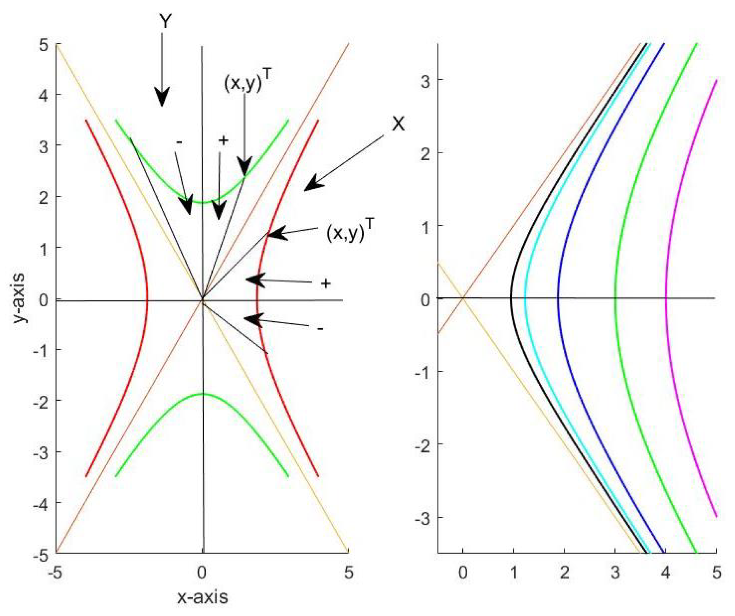
Figure 3.
equals two times the signed area content of the hyperbolic sector with and where .
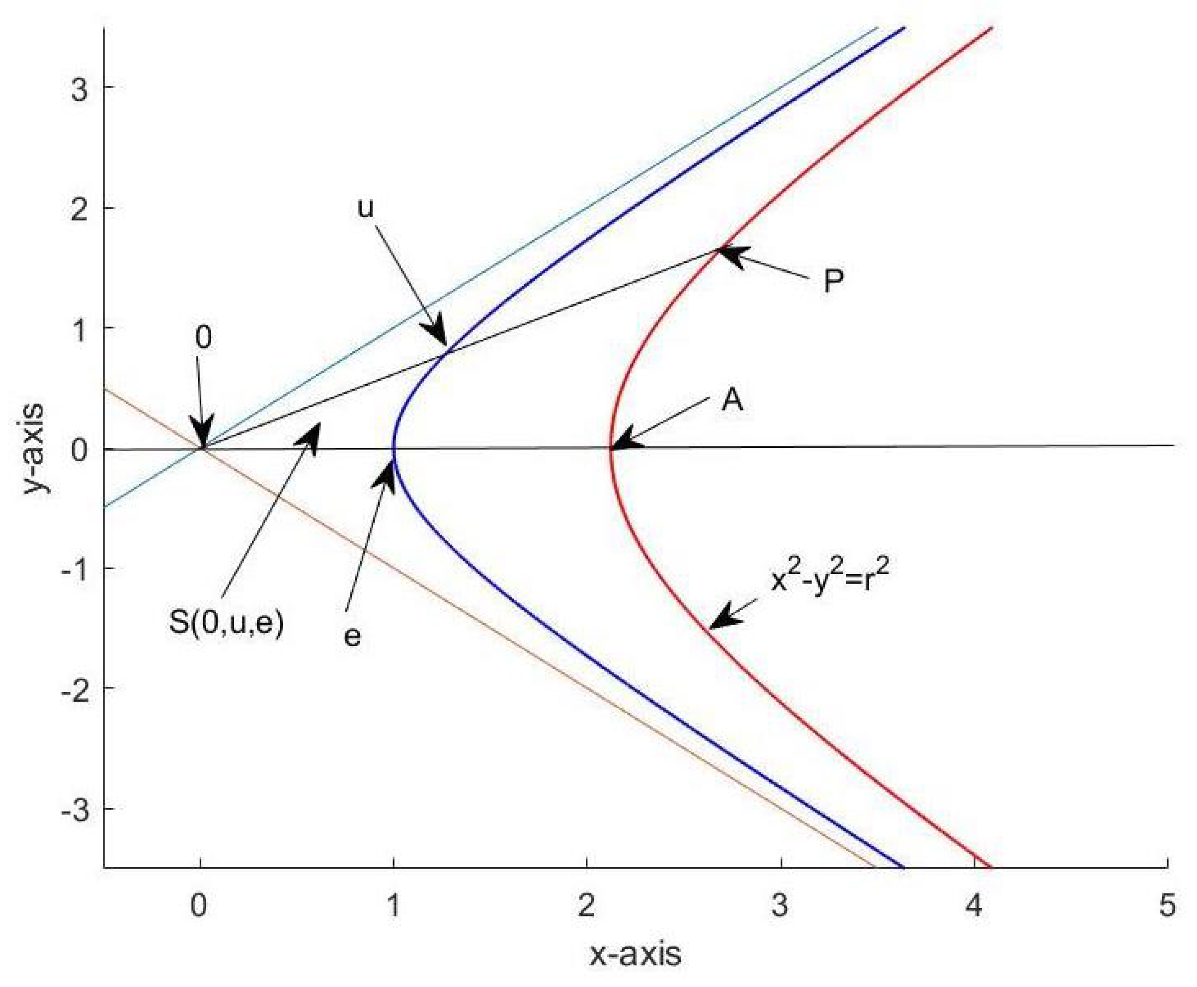
Figure 4.
Hyperbolic vector multiplication within either or means sector combination by adding the signed area contents and multiplying the hyperbolic radii and of sectors and where and .
Figure 4.
Hyperbolic vector multiplication within either or means sector combination by adding the signed area contents and multiplying the hyperbolic radii and of sectors and where and .

Figure 5.
Subtraction of area contents.
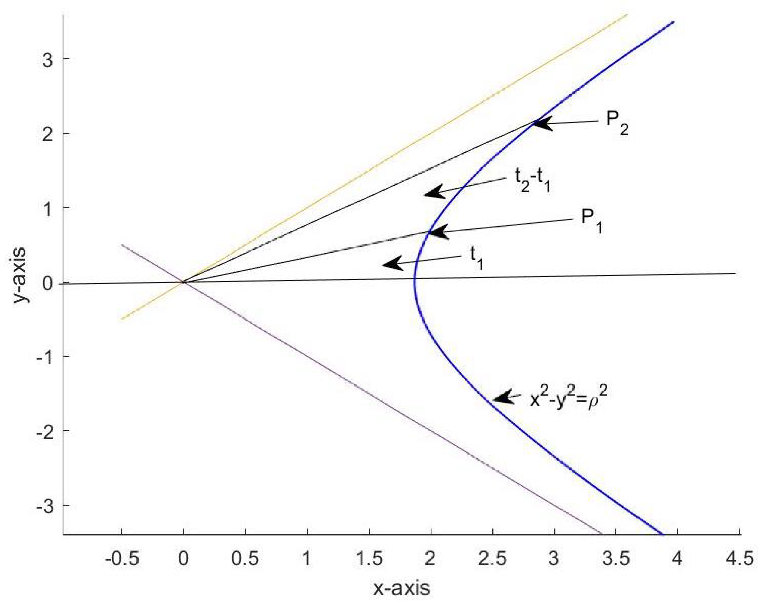
Figure 6.
The solutions of the quadratic vector equation.
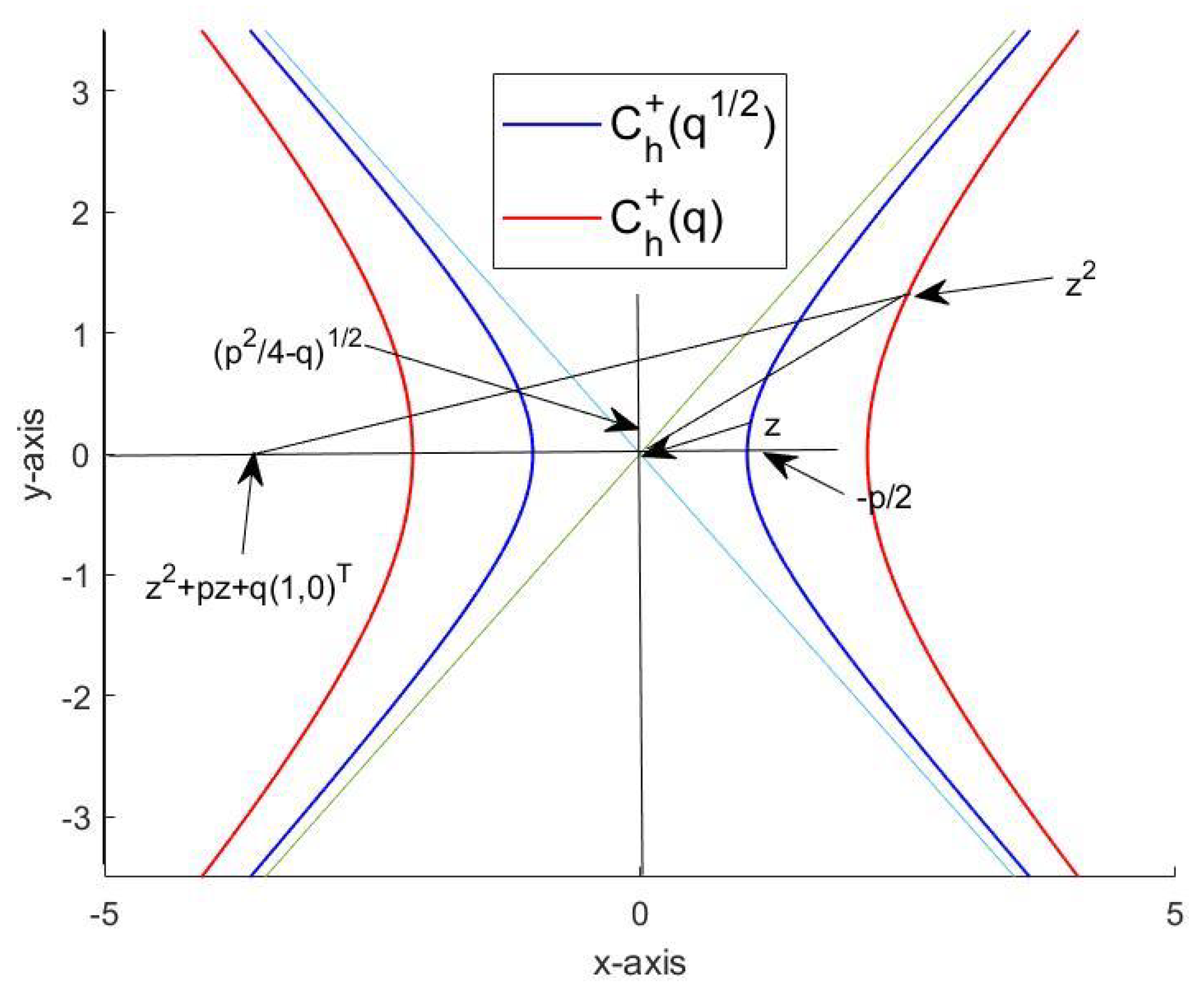
Figure 7.
Signs of area contents.
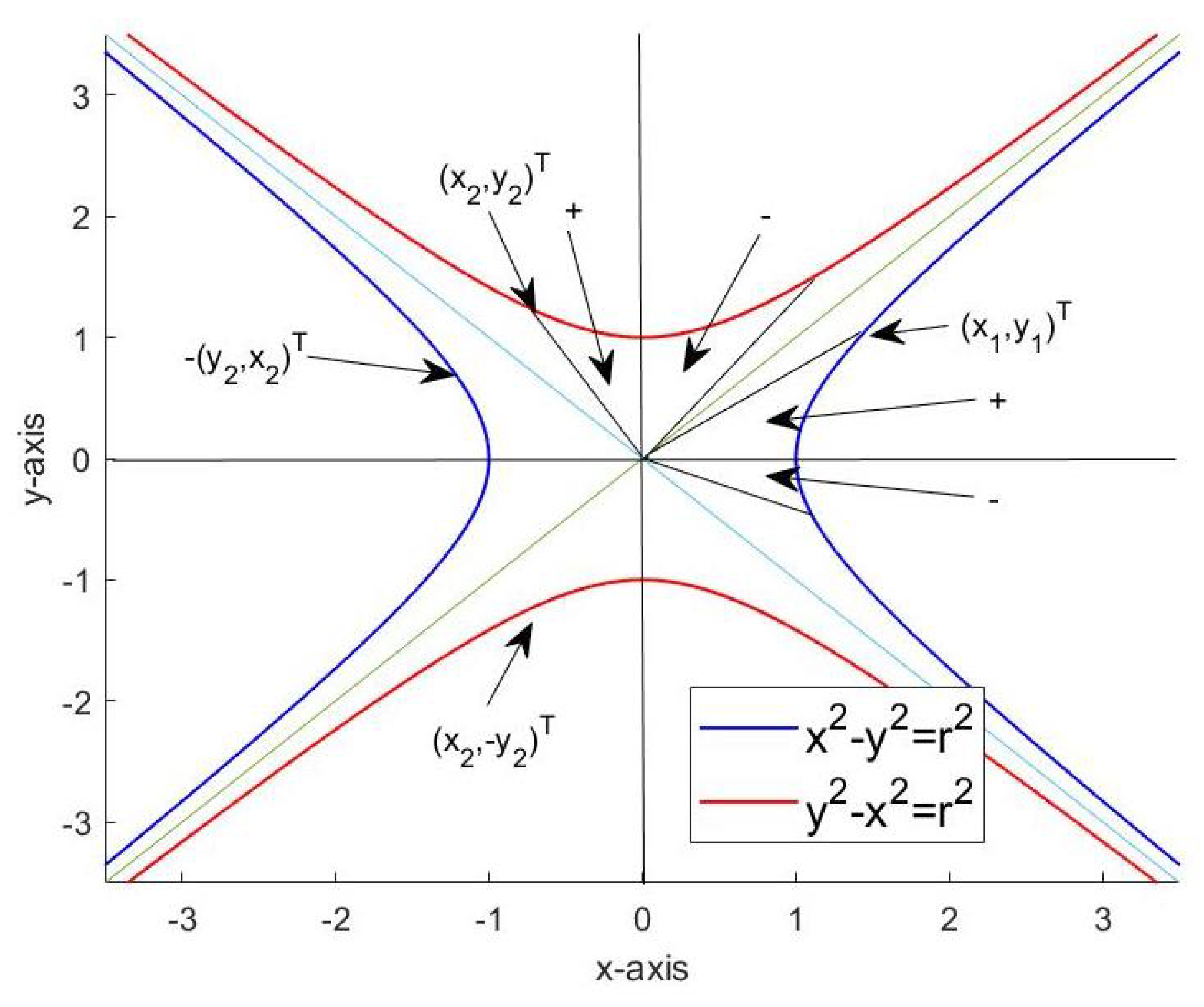
Figure 8.
Three−dimensional space−time: the hyperbola rotates around the axis.
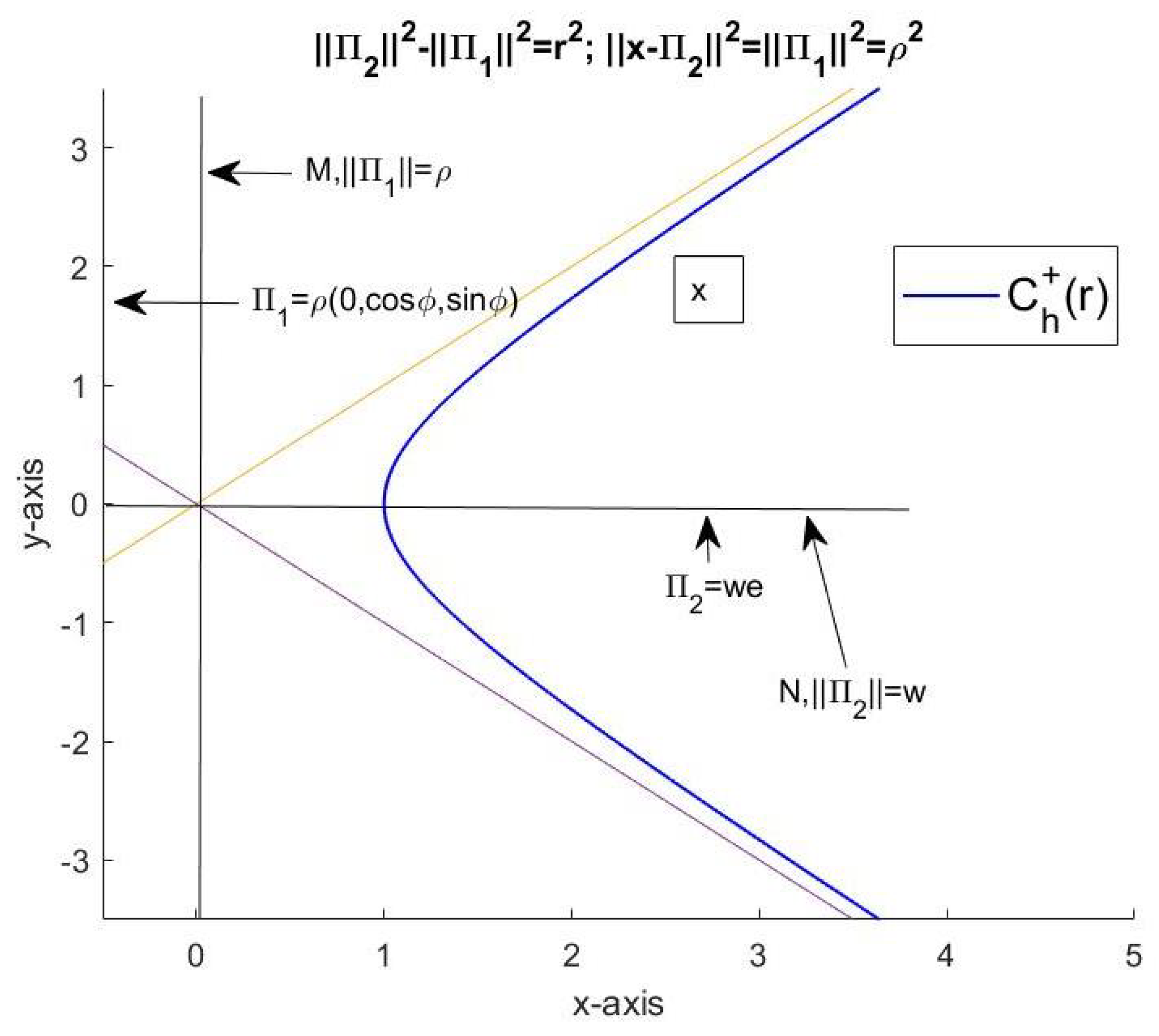
Figure 9.
Sector S belongs to the plane which is spanned up by the vectors and .
Publisher’s Note: MDPI stays neutral with regard to jurisdictional claims in published maps and institutional affiliations. |
© 2022 by the author. Licensee MDPI, Basel, Switzerland. This article is an open access article distributed under the terms and conditions of the Creative Commons Attribution (CC BY) license (https://creativecommons.org/licenses/by/4.0/).
Share and Cite
MDPI and ACS Style
Richter, W.-D. On Hyperbolic Complex Numbers. Appl. Sci. 2022, 12, 5844. https://doi.org/10.3390/app12125844
AMA Style
Richter W-D. On Hyperbolic Complex Numbers. Applied Sciences. 2022; 12(12):5844. https://doi.org/10.3390/app12125844
Chicago/Turabian StyleRichter, Wolf-Dieter. 2022. "On Hyperbolic Complex Numbers" Applied Sciences 12, no. 12: 5844. https://doi.org/10.3390/app12125844
APA StyleRichter, W.-D. (2022). On Hyperbolic Complex Numbers. Applied Sciences, 12(12), 5844. https://doi.org/10.3390/app12125844
Note that from the first issue of 2016, this journal uses article numbers instead of page numbers. See further details here.