RegioRail—GNSS Train-Positioning System for Automatic Indications of Crisis Traffic Situations on Regional Rail Lines

Abstract

The identification of the position of rail vehicles plays a crucial role in the control of rail traffic. Available, up-to-date information on the position of vehicles allows us to efficiently deal with selected traffic situations where the position of vehicles is very important. The main objective of this article is to introduce (i) a concept of a solution for identification of the current position of rail vehicles based on the worldwide-recognized system of the GNSS with the use of an original railway network data model, and (ii) the use of this concept as supplementary support for the dispatcher control of rail traffic on regional lines. The solution was based on an original, multilayer rail network data model supporting (i) the identification of rail vehicle position and (ii) novel algorithms evaluating the mutual positions of several trains while detecting the selected crisis situation. In addition, original algorithms that enable automatic network model-building (on the database server level) directly from the official railway infrastructure database were developed. The verification of the proposed solutions (using rail traffic simulations) was focused on the evaluation of (i) the changing mutual positions (distances) of trains on the railway network, (ii) the detection of nonstandard or crisis traffic situations, and (iii) the results of the calculations of necessary braking distances of trains for stopping and collision avoidance. The above verification demonstrated the good applicability of the proposed solutions for the potential deployment within supplementary software support for real traffic control. The described concept of the supplementary support determined for railway traffic control (using the localization of trains by means of the GNSS) is intended mainly for regional, single-rail lines. This type of line is very often not sufficiently equipped with standard signaling and interlocking equipment to ensure the necessary traffic safety. Therefore, when deploying this support, the new algorithms for the automatic detection of critical traffic situations represent a significant potential contribution to increasing operational safety.

1. Introduction

Identification of the location of rail vehicles plays an essential role in transport systems control. Current information about the location of the monitored elements enables its users to effectively solve situations where transport element position has key importance, [1]. Long-term efforts have been made in railway transport towards the implementation of a harmonized ETCS (European Train Control System) within all the EU member states. The ETCS is a part of the ERTMS (European Rail Traffic Management System), which is designed for railway transport management. The system uses, among others, information about the current, real-time train position. However, there are already various studies on how to adapt the ERTMS using the GNSS [2]. However, the mentioned complex Europe-wide systems are primarily designed for main rail corridors with heavy traffic intensities. Application of the management systems to regional and single tracks is not counted on regarding their low traffic loads. Permanent crisis operational situations have unambiguously demonstrated that the lower frequency of regional and single-track traffic does not essentially reduce the risk of train collisions or nonstandard situations [3,4,5].

With the aim to prevent crisis situations, we must pay attention to the development of systems capable to detect such situations, e.g., identify current positions of rail vehicles with the use of the worldwide GNSS within a multilayer railway network model reflecting the undirected data structure graph. The detection can be carried out either by selected analytical approaches or with the use of artificial neural networks or machine learning [6]. The use of the GNNS in rail transport has been the subject of a number of research studies for many years, focusing on a variety of issues. These have included testing in laboratory conditions [7], establishing methodologies for risk analysis and evaluation of GNSS-based localization systems [8,9] and or detecting train integrity to quantify safety integrity level (SIL) criteria [10]. Additionally, the issues of signal reliability [11,12] and the adaptation of localization systems in case of signal failure [13,14,15] must be addressed when using the GNSS.

In the context of the localization of rolling stock within the combination of the ETCS and the GNSS, the use of so-called virtual balises [16,17] can be mentioned as an alternative to physical balises, e.g., on regional lines.

2. Literature Review

Several different solutions exist that deal with rail vehicle position on regional tracks. The vast majority of these solutions use the GNSS (Global Satellite Navigation System), balises, or odometers. Wireless information transfer is most frequently performed through mobile networks, GSM-R (Global System for Mobile—Railway), or by means of standard GSM technology.

2.1. ERTMS Regional—Sweden

This system was developed in cooperation with the International Union of Railways (UIC); the Swedish Transport Administration, Trafikverket; and with the Bombardier company [18]. ERTMS Regional is a simpler and cheaper version of the ERTMS/ETCS L1 and L2 systems as a suitable option for low-traffic lines. The designed system is operated on a single track of a 143 km overall length with five stations and a density of sixteen trains per day. The UIC plans further extension of the track to a total length of 565 km. The basic principle is a periodic (every 6 s) transmission of information about the train position to the Train Control Center—TCC—which grants the train drive permits. Information about the train position is obtained from an odometer; the position is further specified by means of balises installed at stations and on the track with a fixed spacing of five kilometres. Mobile network GSM-R and GSM are used for the information transfer.

2.2. LOCOPROL—France

Another system that is used in France is the technological solution of LOCOPROL [19,20]—the low-cost satellite-based train location system for signalling and train protection for low-density traffic railway lines. The system was developed by ALSTOM and its partners from Belgium, Germany, and France within a research project focusing on the use of satellite navigation for low-density railway lines. LOCOPROL is used on a single-track line with a 35 km length. Similarly, the main principle is a radio block center (RBC) that collects information about rail vehicle position on the line. The RBC also receives information about the train drive permits. Information about the position is detected by means of GPS, GLONASS, and in the future by Galileo satellite navigation and odometer. Specification of the position at critical points (especially at stations with gridirons or at radio-shadowed areas) is carried out by means of the installed balises. The position locator is integrated directly in the ETCS deck device, using the public operator’s network for information transmission. The train integrity is controlled by its engine driver.

2.3. 3InSat—Italy

The Train Integrated Safety Satellite System—3InSat—was developed in Italy by Ansaldo STS in cooperation with other foreign partners. The project was finalized in 2014, and the designed system is used on a regional single-track line in Sardinia with a total length of 50 km. The system also uses RCB for data collection and for train drive permits. The information about vehicle position is obtained from satellite navigation (GPS EGNOS and Galileo) and from an odometer. GSM, TETRA (Trans-European Trunked Radio) systems, and satellites are used for the transmission of information. The architecture is based on ETCS L2 [21,22]

2.4. SATLOC—Romania

The SATLOC system was designed by the UIC in cooperation with eleven organizations from six countries with the support of the European Space Agency (ESA), Paris, France. The project focused on the development and innovative use of the GNSS for the support of railway transport control on regional lines. The project also aimed to design new operating standards, as well as software and hardware solutions and services. The SATLOC system is now operated in testing mode on a single-track line of 27 km length. The designed and tested system corresponds with the ETCS L2 standards [23,24].

2.5. IDEA Project 52—USA

The IDEA Project 52 [25] for a track maintenance system was designed to localize vehicles with the use of a GPS system and so-called navigation by calculation. The main localization principle is to identify position by means of differential GPS and with Carrier-Phase Differential GPS (CDGPS) algorithm level 2 [26]. This principle works on the basis of raw GPS L-band carrier signals, enabling the determination of the position to an accuracy within centimetres (10–30 cm). The continuously extended High Accuracy—National Differential GPS (HA-NDGPS) equipment is used at stationary differential GPS stations. The position data is then transferred via the communication line to a dispatcher´s site, which allows effective transport control within the maintained track.

The original solution proposed the use of one standard frequency. However, a study [26] demonstrated that, to achieve the required frequency, it was necessary to maintain maximum intervals between the stationary stations of up to 30 km. A dual-frequency (L1/L2) GPS receiver must be used to reach greater intervals between the stationary stations (up to 150 km). A further step to increase the algorithm calculation accuracy was the introduction of the Kalman filter. Distances between the stationary stations, thus, eventually increased to 200 km. However, the required accuracy at these distances (150–200 km) has not been proved.

For the identification of a rail vehicle within infrastructure, a digital track map is used. The identification of a rail on a single track is trivial. The problem turns up in the identification of rail on multirail tracks. This problem is solved by means of a calculation that determines the most presumable rail. The accuracy is 40 cm with a probability of 97%.

2.6. Positive Train Control—USA

Since 2010 (with planned termination in 2015), project Positive Train Control has been carried out in the USA (PTS) [27]. The objectives of the project were the following:

• The detection of train separation or uncoupling and potential collision;
• The tracking of speed enforcement;
• The temporary limitation of speed;
• The safety of railway maintenance crews.

Among the essential prerequisites to achieve the objectives was the employment of a unified, nationwide standard differential GPS, the Nationwide Differential Global Positioning System (NDGPS). As indicated in the previous solution, the system should be based on an accurate localization of railway vehicles by means of differential GPS.

3. Materials and Methods

In this section, we provide data for the description of infrastructure, the design and implementation of a multilayer railway network model, and the algorithms for identification of a rail vehicle position in a rail network and for the calculation of rail vehicle braking distance.

3.1. Description of Infrastructure

The existing monitoring localization systems for railway vehicles often combine GNSS technology with additional systems, e.g., balises (physical or virtual) or odometers, which make the train position more precise and can be used both on multirail tracks and for more precise localization. This article aims to introduce the available localization system for additional support of the dispatcher control based on the GNSS, focusing on regional and single tracks where a certain inaccuracy resulting from the GPS character can be accepted.

The infrastructure of the Czech rail network currently covers over nine and half thousand kilometres of railway lines divided into four categories (Figure 1).

• Corridor lines recorded in the European railway system with a total length of 1402 km (pink color);
• National lines recorded in the European railway system with a total length of 1189 km (green color);
• National lines not recorded in the European railway system with a total length of 3748 km (red color);
• Regional lines not recorded in the European railway system with a total length of 3232 km (blue color).

Single tracks cover approximately 7607 km, which corresponds to a maximum of 80% of the total length. The regional lines cover over 33% of the tracks [28,29].

To build a railway network model, it is inevitable to have suitable data, enabling us to develop a model with a certain degree of abstraction. Experiments have show that a rail network model design can be based on hectometer posts. These devices are physical elements located in the railway infrastructure rail yard (at about 100 m distances). Each of them disposes of a GPS coordinator, among others. Data analysis provided by the Railway Infrastructure Management—Technical Center proved that the following four data tables are generally sufficient for a railway network model design:

• The stationing and hectometric posts table and TUDU (track definition node);
• The supertrack table;
• The railway stations table;
• The definition suprasections table.

The key connection element between individual tables is always the TUDU. We can say that individual supertracks consist of definition supra-sections, where each suprasection contains the track definition nodes (TUDUs) with hectometre posts. The basic aspects of a railway network description are described as a complex in Figure 2.

The hectometer points in Figure 2 indicate the distance in kilometers, and they are marked as grey points in the graph. The TUDUs are recorded by six-digit codes (163105, 163106, 16307, and 173202) and by full lines in the graph (red, black, orange, and brown). Individual suprasections (CLS 007, CLS008, REG023) are marked with a light blue color, and the supertracks by interrupted lines. Significant traffic points (line branching) are marked with a green square.

The above indicated way of viewing infrastructure relates to the situation in the Czech Republic; however, a same or similar attitude or its variations can be applied also outside the country because hectometer posts exist on tracks in many European countries.

3.2. Design and Implementation of a Multilayer Railway Network Model

Based on the relevant data analysis, an original three-layer railway network model was designed, where individual layers enabled the depiction of a different degree of rail infrastructure abstraction. The schematic of the rail line model is shown in Figure 3.

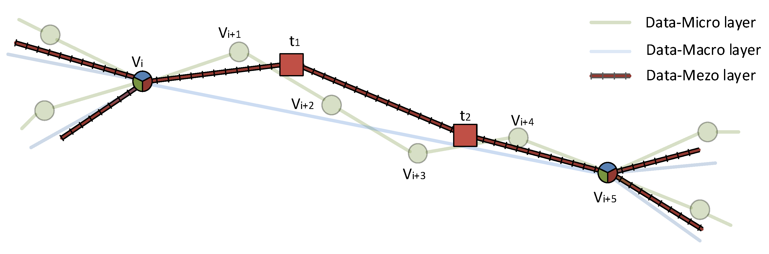
The concept of a three-layer rail network model is presented in Figure 4, where the data-micro layer is depicted in green, the data-mezo in brown, and the data-macro in blue.

It is essential to define the basic variables for the description of an individual algorithm concept, enabling the building of the above-indicated three-layer rail network model. Explanatory notes and the used functions are shown in

Table 1. Explanatory notes.

Used Symbol	Description
$h=\left(h^0,h^{gps},h^{tudu}\right)$	Hectometer post (vertex) h is described as an arranged triplet, where $h^0$ is a kilometric value of the position, $h^{gps}$maintains the GPS position coordinates, and $h^{tudu}$ corresponds to the TUDU identification of a corresponding hectometer post.
$H=\underset{i\in I}{{\displaystyle \cup }}{h}_i$	Set of all the hectometer posts, where I is an index set of hectometer posts.
$D_i=\{h | h\in H\}$	Set of an ith TUDU consisting of hectometer posts.
$D=\underset{i\in I}{{\displaystyle \cup }}{D}_i$ $\forall D_i,D_{j }\in D ;i\ne j;$ $i,j\in I:D_i{\displaystyle \cap }{D}_j=\varnothing$	Set of all TUDUs, where I is an index of the TUDU set.
$N=\{n | n\in D\}$	Set of suprasections (TDNU) consisting of TUDU.
$S=\{s | s\in D\}$	Set of all supertracks consisting of TUDU.
$S^N=\{s^N | s^N\in N\}$	Set of all supertracks consisting of TDNU.
$Y=\{y |y=\left(h,d\right);$ $h\in H;d\in D\}$	Set of all switch-points determined by hectometer posts and TUDU.
$h_1⊝h_2$	Two different hectometer posts are in the same TUDU: $h_1\in d \wedge h_2\in d; h_1\ne h_2; d\in D$.
$h_1\odot h_2$	Two different hectometer posts are in different supertracks:$h_1\in S_1 \wedge h_2\in S_2 ;h_1\ne h_2 ; S_1,S_2\in S; S_1\ne S_2$.
$V$	Set of all trackage model vertices (in data-micro layer).
$E$	Set of all edges in the track yard model (in data-micro layer).
$V^S\subset V$	Set of super-vertices (in data-macro layer).
$E^S\subset \left(V^S\times V^S\right)$	Set of super-edges (in data-macro layer).
$t=\left(t^0 ,t^{gps},t^{tudu}\right)$	Railway station $t$ is represented as an arranged triplet, where $t^0$ is a kilometric value of the station position, $t^{gps}$is the GPS position of the station, and $t^{tudu}$ is the identification of the corresponding TUDU.
$T=\underset{i\in I}{{\displaystyle \cup }}{t}_i$	Set of all stations, where I is an index set of stations.
$V^M=\left(V^S{\displaystyle \cup }T\right)$	Set of meso-vertices.
$E^M\subset \left(T\times V^S\right){\displaystyle \cup }$ $\left(V^S\times T\right){\displaystyle \cup }\left(T\times T\right)$	Set of meso-edges.

and

Table 2. Functions.

Subprograms and Functions	Specification
setData ( $\downarrow \uparrow h_j^{’},\downarrow H_j^{origin}$ )	The values of the GPS coordinates of the new substitution hectometer posts correspond to the arithmetic means of the values of the respective coordinates of all of the hectometer posts from set $H_j^{origin}$. If at least one of the hectometer posts out of the set $H_j^{origin}$ bears the sign of a point, then the new continuous hectometer post also bears the sign of a point. We adopt further information about the hectometer post from a random hectometer posts from the set $H_j^{origin}$ in which the hectometer post is located.
findShortestRoute$(\downarrow h^{start}$$, \downarrow h^{end},\uparrow E^{temp}$)	Between its outer super-vertices, $h^{start}$ and $h^{end} ,$we find, using the shortest route search algorithm (in the data-micro layer), a set of part edges $E^{temp}$.

.

3.2.1. Methodology of Data-Micro Model Layer Construction

The first data layer (data-micro) reflected the physical rail network infrastructure with the minimum degree of abstraction, while individual model and graph vertices corresponded to stationing.

Substitute Rails and Hectometer Posts

Data imported from the input sets unfortunately do not fully reflect the real form of the rail network infrastructure, especially at multiple-line stations. In the case that a station has ten rails (standard and dead-end rails), the input datasets may contain, for example, only three rails. In most cases, the station rails do not converge in any way and continue to the next station.

Generally, the TUDU markings of a rail line section change, among others, before and after a station (as a part of the deviated tracks). This means that each station has (with certain exceptions) a unified TUDU marking along the whole length. The same refers to stations with more rails, that is, at each through-running station, the TUDU markings change at the deviated tracks before and after the station.

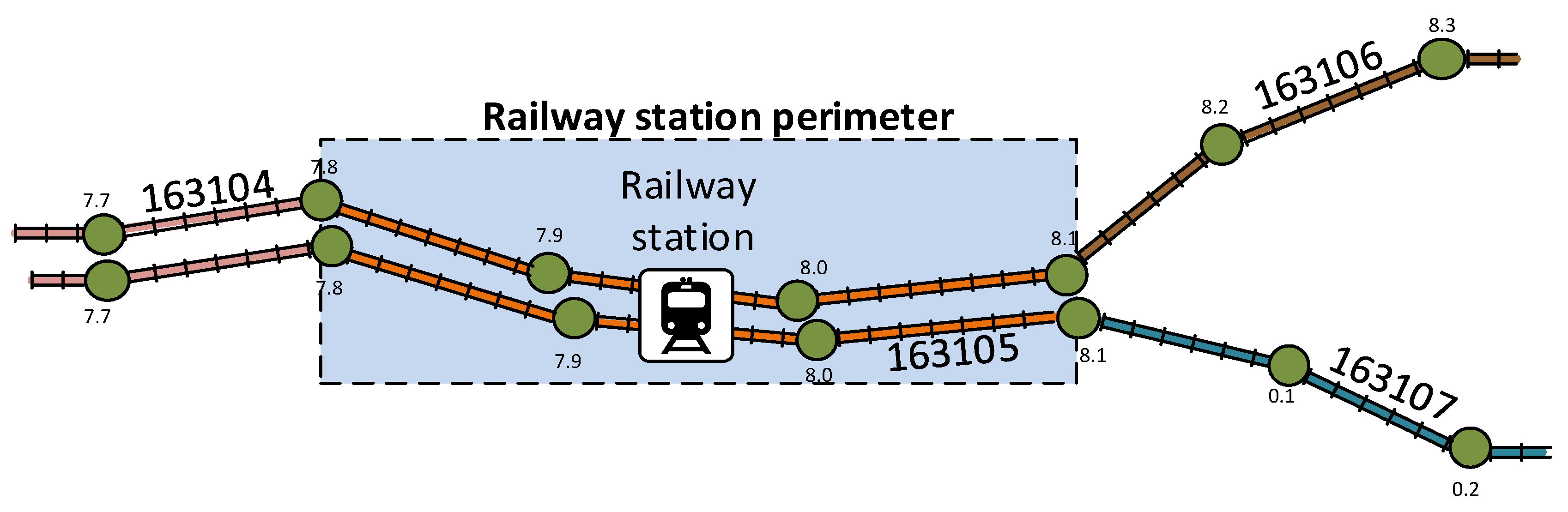
It is important that each of the rails has an identical marking to the TUDU of the neighbouring rails that run through the station and that hectometer posts in the same TUDU have the same kilometric value at each rail (Figure 5).

Regarding the above-indicated facts, we decided that, for the model design, the rails in multiple-line stations would be unified into a so-called substitute rail. This ensured, among other things, the convergence of all the rails before the station into one rail and, consequently, optional division of the substitute rail into more rails after the station.

The model, thus, made it possible to return to any other departure direction from any arrival direction in the same way as real operation. For this purpose, it was necessary to calculate the new substitute hectometer posts (the calculation is shown below within Algorithm 1—Arrangement of sets of vertices within individual TUDUs), which formed vertices belonging to one substitute rail (Figure 6).

In the process of making substitute rails, we needed to consider a situation when one substitute rail was not permissible. This can mainly happen at smaller stations on multiline tracks that have no switch along the whole length; therefore, it is impossible to travel from one line to another.

The collected data also contained information about the positions of individual switch-points on the line; that is, we could detect a switch-point’s presence in the given station or vertex and decide whether a substitute line must be constructed.

Another specific requirement of a multiline track was keeping the structure of individual lines crossing outside stations (by switch-points enabling passing from one line to another. The performed examinations demonstrated that rail line sections enabling such crossing had their own TUDU marking, which mostly contained only one or two hectometer posts. Due to this fact, we used the same algorithm for maintaining the line structure as that for the substitute line at stations, i.e., forming a substitute line along all the hectometer posts on the line section marked with the same TUDU.

Generally, the methodology for building the lowest layer can be summarized in three basic steps:

• The formation of vertices within one TUDU (Algorithm 1);
• The construction of edges within one TUDU (Algorithm 2);
• The formation of edges between neighbouring TUDUs (Algorithm 3).

Algorithm 1: Formation of a vertex set within individual TUDUs.

The results of the given algorithm are described in Figure 7 in a simplified way.

Algorithm 2: Construction of edges within one TUDU.

The results of the algorithm are presented in Figure 8.

Algorithm 3: Formation of edges between neighbouring TUDUs.

The resulting situation is shown in Figure 9.

3.2.2. Methodology of Data-Macro Model Layer

Another layer of the railway network model was the data-macro layer. Typical for the greatest degree of abstraction, it derives from the first data-micro layer, introducing a greater granularity. We introduced the terms super-edge and super-vertex on this level.

A super-vertex was a vertex of the data-micro layer that was incident with more than two edges.

A super-edge connected two super-vertices. In other words, it replaced the hierarchy of edges in a micro-layer in a section where lines did not cross, converge, or divide into one or more lines, Algorithm 4.

Algorithm 4: Algorithm concept of data-macro model layer.

The results of the algorithm are shown in Figure 10.

3.2.3. Methodology of Data-Meso Model Layer Construction

An evaluation of the edges in the first data layer (data-micro) corresponded with lengths of 100 m, while in the second data layer with a higher degree of abstraction (data-macro), the edge evaluations reflected distances of several tens of kilometers. Both the data layers (data-micro and data-macro) did not directly involve railway stations as their vertices, e.g., the determination as to whether a rail vehicle is or is not at the station, or the use of the distance from the station as an alternative solution (by means of station-relating TUDU identification). This fact took into consideration the third data layer (data-meso) by means of individual super-edge decomposition, Algorithm 5.

The above-mentioned data layers (data-micro and data-macro) used the same database for the vertices (hectometer posts), while another vertex type was integrated in the new data-meso layer. This vertex type represented individual railway stations. On this level, we introduced the terms meso-edge and meso-vertex.

• Meso-vertex was represented by (i) the super-vertex or (ii) a railway station;
• Meso-edge was the marking for an edge that connected meso-vertices.

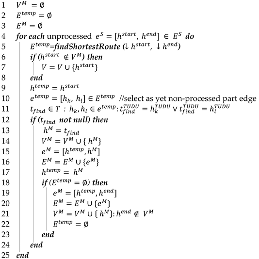
Algorithm 5: Algorithm concept of data-meso model layer construction.

The results of the described algorithm are in Figure 11.

The introduction of a multilayer railway network model enabled us to use a different scope of abstraction for different application attitudes, such as monitoring the current position of a rail vehicle on a single track and periodical evaluation of this position in relation to other moving transport elements. The data layers of the mezo or macro models were suitable for the monitoring of this type of rail vehicle. Should we need to consequently evaluate the mutual positions (distance) of two vehicles, the data-micro model seemed more suitable.

3.3. Identification of a Rail Vehicle Position in Rail Network

As the above-indicated research demonstrates, a number of localization systems exist in the world based on the GNSS. However, these systems are often complemented by further elements which participate in the resultant localization. This is why a mere GNSS-based localization may not be considered original; we have to take into view the overall localization system concept using the GNSS as a general supplier of information about a rail vehicle position and its consequent connection with the designed railway network model. This is one of the reasons why this article puts stress on the algorithms and methodology of building a railway network model, as well as on the proper description of localization and its use in the detection of nonstandard situations for the additional support of rail transport control by dispatchers.

It was possible to build a three-layer railway network model from the above-indicated algorithms with different abstraction levels. The final model was then saved in the Oracle database with a Network Data Model (Oracle Spatial and Graph) superstructure, which enabled the building of a graph representation directly on the database level. For the correct functioning, the database structure must be complemented by binding tables to maintain individual layer hierarchies. The vertices and edges of the graph were saved in predefined database tables and complemented by the appropriate geometric properties (point, right line), which were saved in a special object–relation data type, SDO_GEOMETRY. The vertices were represented by multidimensional points with GPS coordinates. The edges were carried out as line segments between the relevant vertices. For effective work with this object–relation data type, Oracle offers several functions and operators, such as a calculation of distance between two objects, a search for the object closest to the given object (e.g., a point), or finding an intersection of two geometric objects.

The design of the actual access of a rail vehicle localization access on the track was based on the correct match of GPS information about the vehicle position (obtained from the communication terminals installed on a rail vehicle) with the nearest vertex and edge of the graph. The found vertex (hectometer post) then disposes of a multidimensional key in the form of a GPS coordinate and is linked to other railway-infrastructure-relating information by means of definition section of TUDU.

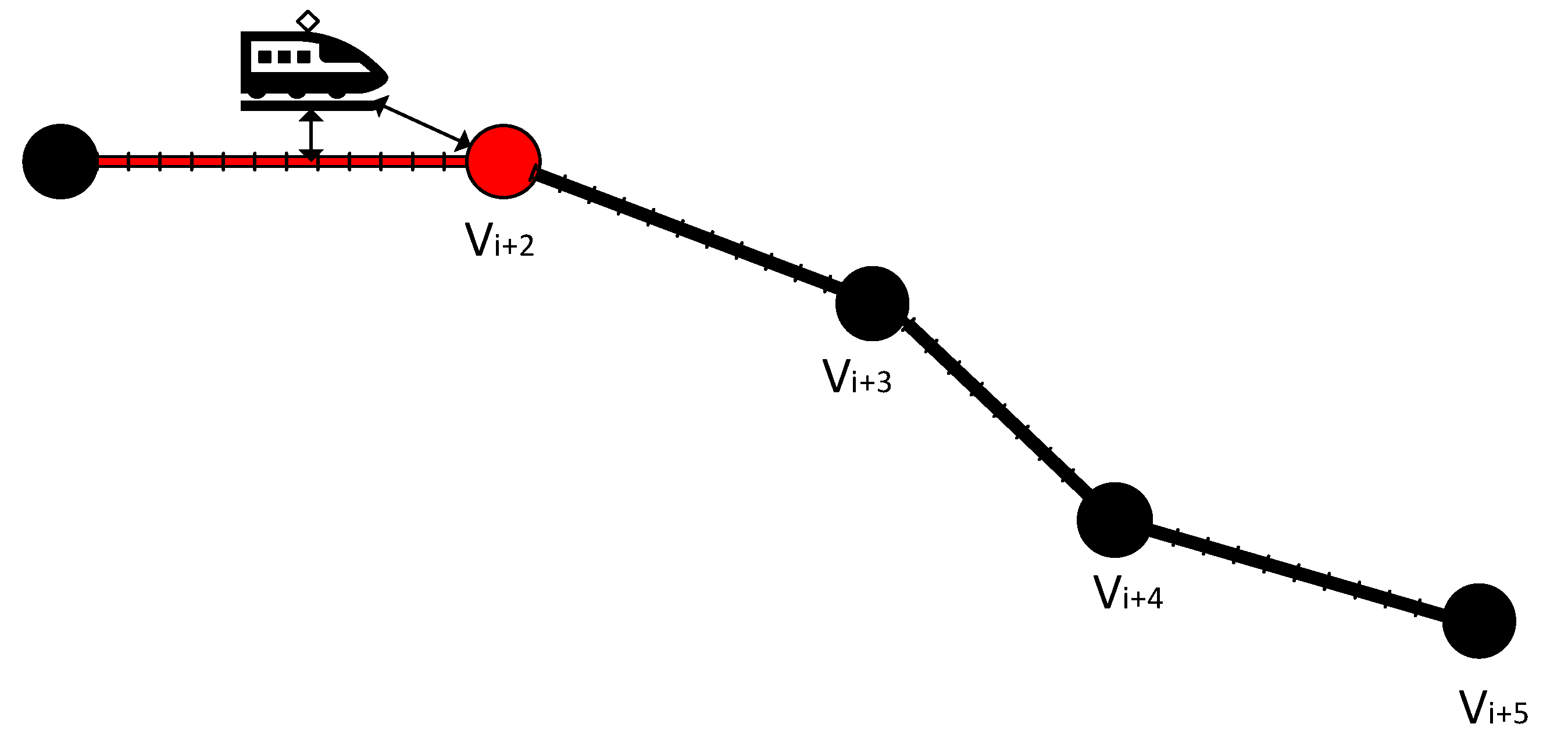
To carry out the actual rail vehicle localization access, we used an SDO_NN (nearest neighbour) operator [30], which looked for a geometrical object closest to the given object (e.g., a point). In other words, the nearest vertex or model edge could be found in the current rail vehicle position (Figure 12).

The actual detection of the current rail vehicle position was divided into the following steps:

• Search for the nearest graph vertex and edge—from the current rail vehicle position regarding the three-layer railway infrastructure model.
• Evaluation of the relevant incoming GPS information from the communication terminal—verification as to whether the current position was loaded by an excessive error. The verification included the following assessments:
  • The distance of a rail vehicle from the nearest vertex or edge and its admissibility within the determined tolerance.
  • Was the current position related to the same supra-edge as in the previous positions on the condition that it was expected to occur on it?
  • Was the azimuth of a rail vehicle motion’s direction within the admissible tolerance?
    In the event that the current position failed to meet some of the above indicated criteria, the position was considered invalid.
• Calculation of the accurate rail vehicle position on a model edge—by means of perpendicular point projection (the current vehicle position) on a right line (an axis of the found edge or rail).

In the event of current position information failure or invalidity (see above), a new current position was extrapolated based on the last position’s historical data. The last known position was used for the calculation of the extrapolated position:

• Vehicle speed;
• Vehicle azimuth;
• Rail azimuth.

Based on this data, we calculated a new fictive rail vehicle position that could, for a certain period, substitute the real vehicle position, enabling us to use the designed system for short-term or extraordinary failure of the supplied information about the current position of a vehicle.

3.4. Nonstandard State Detection

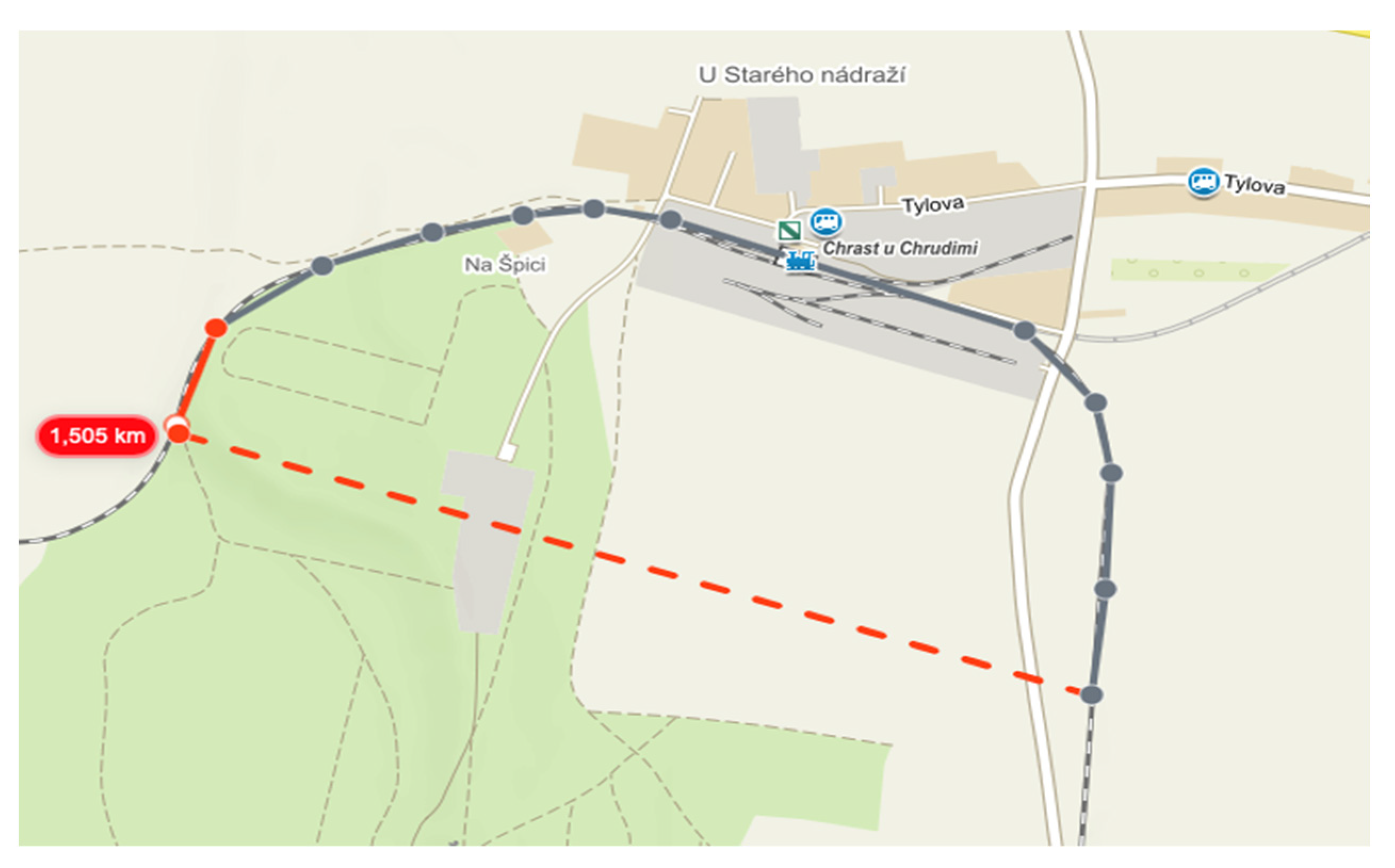
We can see a long-term trend in railway transport to implement a unified European Train Control System (ETCS) within all the EU member countries. However, the complex Europe-wide systems are primarily designed for main railway corridors with high traffic intensities. The application of the above-mentioned control systems on regional and single lines is currently not counted on (regarding their low capacities). The continuing occurrence of crisis operational situations has proved that the lower frequency of regional and single lines does not significantly reduce the risk of train collision or nonstandard situation occurrence. Generally, nonstandard or crisis situations within single lines can be considered as situations when two rail vehicles (trains) are located within an under-the-threshold distance. The easiest solution seems to be testing of the air distance; nevertheless, this solution has certain limits, e.g., in line crossings or on a non-linear line course (see Figure 13).

The above-indicated example clearly shows an unsuitable access of air distance in relation to the line profile. The real distance (grey curve) is 2.251 km, while the air distance of the monitored rail objects (red interrupted line) corresponds to 1.514 km, which is almost 0.737 km less than the real length.

For a more realistic calculation of the distance between two rail vehicles, a multilayer rail network model reflecting an undirected graph combining the data-micro and data-meso layers was used. The data-meso layer was used for the detection of nonstandard situations that were divided into three groups:

• Opposite direction train driving;
• Parallel train driving;
• Moving vs. non-moving trains.

It was vital to differentiate situations when two vehicles were located on:

• One or an identical edge,
• Two neighbouring edges when the incidental vertex of the two edges did not dispose of any track branching or vehicle crossing (e.g., stations).

Both situations are demonstrated in Figure 14 and Figure 15.

The data-micro layer was then used for the calculation of the physical distance between two monitored rail vehicles. This data layer had the lowest degree of abstraction, where each edge corresponded to a length of 100 m.

3.5. Calculation of Rail Vehicle Braking Distance

The dynamics of rail vehicles or vehicle set driving involve several of aspects that can influence several parameters of the drive. These involve, especially, (i) the technical parameters of a train set (e.g., rail vehicle acceleration or overall weight of the set) and (ii) railway infrastructure (track profile, speed limits, etc.)

Reduced Track Profile

Railway infrastructure is a very complex issue involving several parameters that can influence a rail vehicle’s dynamics, as well as its energy aspect [31,32,33]. The real track profile in a common traction calculation was substituted by a reduced set of temporary gradients, the so-called track resistance, which included resistance to:

• Gradient;
• Curve;
• Tunne.

Curve resistance $s{l}_c$was replaced by a fictive upward gradient where, for subsidiary and regional lines, the curve gradient R < 300 m was described by the following relation:

$$s{l}_c=\frac{500}{R-30} [‰]$$

(1)

The reduced gradient $s{l}_r$was then determined by the following relation:

$$s{l}_r=\frac{s{l}_1{l}_1+s{l}_2{l}_2+\dots s{l}_k{l}_k+s{l}_{c1}{l}_{c1}+\dots +s{l}_{cm}{l}_{cm}}{l_1+l_2+\dots +l_k} [‰]$$

(2)

where:

• $s{l}_1$–$s{l}_k$ is thereal gradient in permille (upward gradient “+”, descending gradient “−“);
• $s{l}_{c1}$–$s{l}_{cm}$ are the fictive gradients replacing curve resistance;
• $l_1$–$l_k$ is the gradient length $s_1$to $s_k$ in meters;
• $l_{c1}$–$l_{cm}$ is the curve length up to 1 m.

The condition $(l_1+l_2+\dots +l_k)\le 2,5 \left(l_{c1}+l_{c2}+\dots +l_{cm}\right)$ must hold.

A sample reduced track profile is illustrated in Figure 16, where arrows show the intended train drive. The data then described the following:

• Kilometric position of a profile change $\left[\mathrm{km}\right]$;
• Direction, where:

  ○

  $“+”$ is a change in the direction;

  ○

  $“-”$ is a change against the direction.

• Track resistance $[‰]$, where:

  ○

  Positive value is an upward track gradient;

  ○

  Negative value is a descending track gradient.

4. Results

In this section, we first focus on the dynamics of the train during braking with the utilization of a reduced track profile and then on the detection of nonstandard situations using computer simulation, which induced the operation of rail vehicles.

4.1. Rail Vehicle Braking

The braking of a rail vehicle or a train set is mainly influenced by:

• The power car technical parameters (negative acceleration);
• The number of vehicles in the set;
• The overall weight of the train set;
• The track profile.

If we consider, e.g., a train set with the following parameters:

• Acceleration: 0.56 m/s²;
• Length: 52 m;
• Weight: 107 t.

Then, for this train set, we can obtain negative acceleration (braking) values by means of a special software tool for the simulation of train dynamics [34], as shown in Figure 17.

The above-indicated graph shows that the measured deceleration for a descending track profile could be approximated by the following linear equation:

$$y=-0.0899x+0.5499$$

(3)

at the reliability of R² = 0.99996.

If we applied the measured deceleration data for an upward-gradient track, then the approximation resulted in the following linear equation:

$$y=0.0887x+0.5499$$

(4)

at the reliability of R² = 0.99974.

To calculate the braking distance, we applied general equations for a uniformly decelerated lineal motion, i.e., relations resulting in the following:

$$v=v_0+at ⟹ t=\frac{v-v_0}{a}$$

(5)

$$s=v_{0}t-\frac{1}{2}a{t}^2$$

(6)

If we subsequently considered the speed of a selected set as $65\frac{\mathrm{km}}{\mathrm{h}}$, then by applying relations (3)–(6), the braking distance of the train set (s) corresponded with the values in

Table 3. Time and length of the braking distance.

Track_Resist [%]	a [m·s−2]	t [s]	s [m]
−2	0.7374	24.49	219.69
−1.5	0.6931	26.05	233.75
−1	0.6487	27.83	249.73
−0.5	0.6044	29.88	268.06
0	0.5600	32.24	289.29
0.5	0.5151	35.06	314.53
1	0.4701	38.41	344.64
1.5	0.4252	42.47	381.04
2	0.3802	47.49	426.09

. Further monitored parameters were negative acceleration or deceleration (a) and time (t).

4.2. Detection of a Train Position

For the detection of nonstandard situations, we used a computer simulation that induces rail vehicle operation.

The designed testing tool contained a core discrete simulation cooperating with a standard calendar of the processor messages performed according to the time stamp. The simulator used data resulting from a real situation based on the processing of historical data of passing trains and generated data. These data were obtained based on cooperation with the Czech state enterprise: Railway Infrastructure Administration (SŽ, s.o.). Our attention in the next experiment was focused on the opposite direction of two rail sets of the same type, while evaluating the following parameters:

• Mutual position (distance) of the two vehicles at the time of detection of a nonstandard situation;
• Braking distance and mutual position (distance) after the two vehicles stopped.

The experiments were processed for the selected time periods when the vehicle sent its current position:

• 5 s;
• 10 s;
• 30 s;
• 60 s.

If we focused on the opposite drive detection on an identical rail or edge (according to the procedure displayed in Figure 14), then their mutual positions (distance) at the time of the detection could be statistically expressed, as shown in

Table 4. Resulting distances [m] at the time of detection of two trains on an identical edge.

	Period 5 [s]	Period 10 [s]	Period 30 [s]	Period 60 [s]
Min	1000	1000	600	0
Max	2500	2500	2400	2400
Average	2016	1968	1628	1140
Median	2100	2100	1800	900
Standard deviation	396.67	413.49	519.63	726.64

.

Table 4 shows that the average and median decreased with the growing time frequency, while the standard deviation increased. The frequency of 60 s was clearly unsuitable: in two cases, there was a collision.

In the second case, opposite drive detections were evaluated at two adjacent rails or edges, according to the procedure shown in Figure 14. The results are presented in

Table 5. Resulting distances [m] at the time of detection of two trains on two neighbouring edges.

	Period 5 [s]	Period 10 [s]	Period 30 [s]	Period 60 [s]
Min	2500	2500	2000	1400
Max	3900	3900	3600	3600
Average	3084	3064	2776	2624
Median	3000	3000	2700	2700
Standard deviation	402.67	418.45	443.87	612.32

.

Table 5 demonstrates that, compared to the first experiment results (Table 2) where the median and standard deviation values were roughly double the value, we saw significantly smaller differences in the distances of all the monitored parameters.

For simplification, in the opposite train drive, we assumed identical speeds of both train sets and equal track value resistance in which a nonstandard situation was detected. The overall braking distance was, thus, obtained with the sum of the partial braking distances for the monitored track resistance, for the upward gradient, or for the downward gradient. The braking-time values (t_sum) and distances (s_sum) of both train sets for the speeds of $65\frac{\mathrm{km}}{\mathrm{h}}$ and $75\frac{\mathrm{km}}{\mathrm{h}}$ are indicated in

Table 6. Time and length of braking distance up to stopping of both train sets.

$\mathbf{Track}\_\mathbf{Resist} [‰]$	t_sum_65 [s]	s_sum_65 [m]	t_sum_75 [s]	s_sum_75 [m]
0	64.48	578.57	74.40	775.05
0.5/−0.5	64.93	582.59	74.92	780.43
1/−1	66.24	594.34	76.43	796.17
1.5/−1.5	68.52	614.79	79.06	823.57
2/−2	71.98	645.78	83.05	865.08

.

5. Discussion

The use of the GNSS in the area of rail transport is a subject of ongoing research. A number of publications have been devoted not only to the application and adaptation of this technology in connection with the localization of rolling stock, but also to its reliability and accuracy. However, in spite of significant advances in research, it has not yet been possible to fully implement this technology in the field of rail transport safety, which may include the ETCS. On the other hand, the GNSS has been used successfully in rail transport for many years, especially in areas where the error inherent in the GNSS can be accepted. This includes, for example, supplementary systems to support traffic control on regional and single-track lines. The frequent occurrence of emergency traffic situations clearly demonstrates that regional lines with lower traffic rates do not substantially reduce the risk of train collisions or abnormal situations.

One of the main objectives of the presented work was the proposal of a suitable methodology for the construction of an original multilayered model of a railway network, where the individual layers of the model reflected the railway infrastructure in different degrees of abstraction. Despite a number of constraints in the input data, a set of algorithms for the automatic generation of a multilayer model (represented by an undirected graph) reflecting the individual hectometers of the railway network was successfully designed. The hectometers were physically located in the railway infrastructure (at intervals of about 100 m), and GPS coordinates were available for each of them.

As the above-indicated research demonstrated, several localization systems exist in the world based on the GNSS. However, these systems are often complemented by further elements that participate in the resultant localization. Therefore, a mere GNSS-based localization may not be considered original; we have to take into view the overall localization system concept using GNSS as a general supplier of information about a rail vehicle’s position and its consequent connection with the designed railway network model. This is one of the reasons why this article put stress on the algorithms and methodology of building a railway network model and on the proper description of localization and its use in the detection of nonstandard situations for the additional support of rail transport control by dispatchers.

The actual detection of the current position of the railway car is based on finding the nearest vertex and edge of the graph and calculating the exact position of the car relative to the corresponding edge of the model. The detection of the current position includes the evaluation of the relevance of incoming GPS information from the communication terminal.

To detect nonstandard or risky situations in rail transport, there is a long-term trend of introducing a single European Train Protection System (ETCS) within all the EU member countries. However, complex Europe-wide systems are primarily designed for main railway corridors with a high traffic intensities. The application of the above-mentioned control systems on regional and individual lines is not currently envisaged (given their low capacities). The continuing occurrence of crisis operational situations has proved that lower frequencies on regional and individual lines do not significantly reduce the risk of train collisions or nonstandard situations.

For a more realistic calculation of the distance between two rolling stocks, a multiayer rail network model reflecting an unoriented graph combining the data-micro and data-meso data layers was used. Attention was paid when two vehicles were located on:

• One or an identical edge;
• Two neighbouring edges when the incidental vertex of the two edges did not dispose of any track branching or vehicle crossing (e.g., stations).

For the detection of nonstandard situations, we used a computer simulation that induces rail vehicle operation. A reduced track profile was used to calculate the dynamics of the rolling stock. A reduced track profile was used to calculate the dynamics of the rolling stock, which replaced the complex properties of the railway infrastructure.

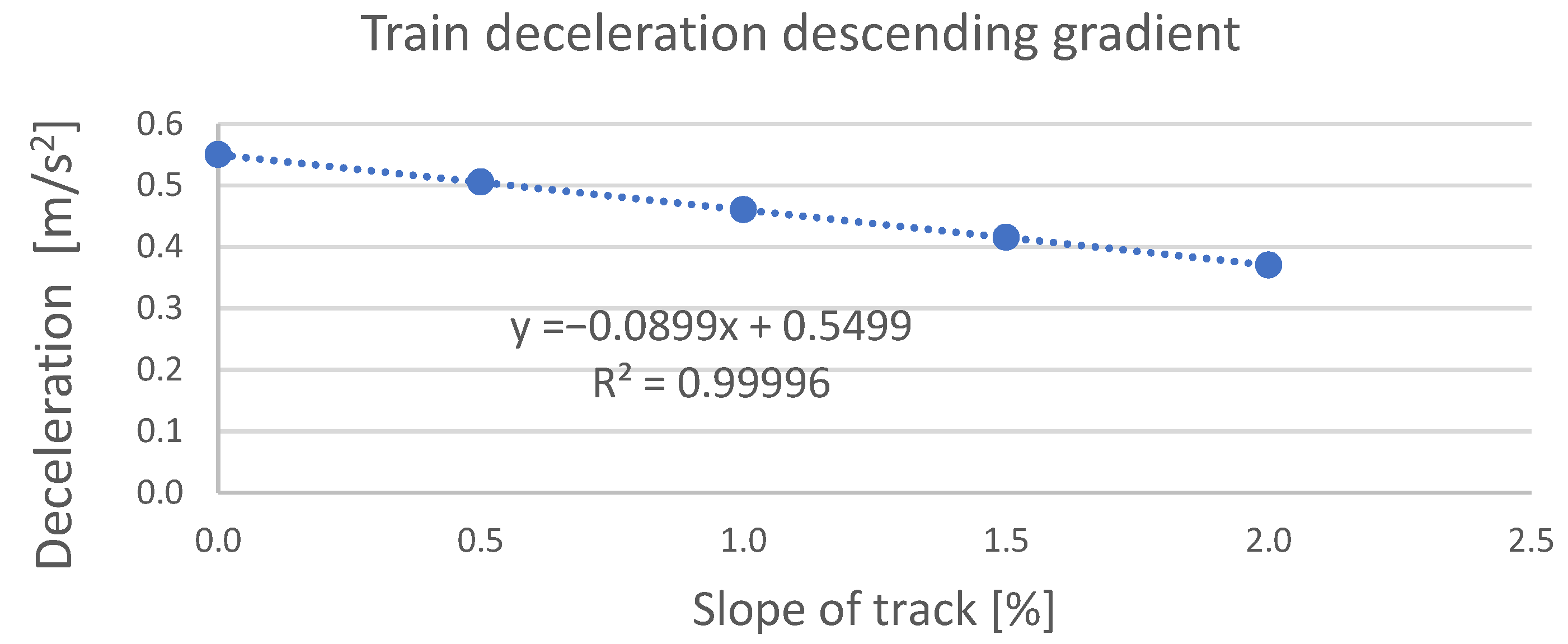
From the measured values obtained in Section 3, it was concluded that, for the simplified dynamics of rolling stock, it was possible to assume a linear approximation with a reliability of R² = 0.99996 negative acceleration for a descending track profile, or of R² = 0.99974 negative acceleration for an ascending track. If we subsequently considered the speed of a selected set as $65\frac{\mathrm{km}}{\mathrm{h}}$, then by applying relations (3)–(6), the braking distance of a train set (s) corresponded with the values in Table 3. Further monitored parameters were negative acceleration or deceleration (a) and time (t).

Within the experiments, attention was focused on the opposite direction of two track sets of the same type when evaluating the following parameters:

• Mutual position (distance) of the two vehicles at the time of detection of a nonstandard situation;
• Braking distance and mutual position (distance) after the two vehicles stopped.

Table 3 demonstrates that, compared to the first experiment results (Table 2) where the median and standard deviation values were roughly double the value, we saw significantly smaller differences in the distances of all the monitored parameters.

For simplification, in the opposite train drive, we assumed identical speeds of both train sets and equal track value resistance in which a nonstandard situation was detected.

The overall braking distance was, thus, obtained by the sum of the partial braking distances for the monitored track resistance, for the upward gradient, or for the downward gradient. The braking-time values (t_sum) and distances (s_sum) of both train sets for speeds of $65\frac{\mathrm{km}}{\mathrm{h}}$ and $75\frac{\mathrm{km}}{\mathrm{h}}$ are indicated in Table 4, which shows that, if the speed was increased by 15%, then the overall braking distance of both train sets increased by 34%. It was also demonstrated that, for the identification of nonstandard situations on an identical edge at the train set speed of $65\frac{\mathrm{km}}{\mathrm{h}}$, the 30 s period of current position detection was sufficient. However, for a speed of $75\frac{\mathrm{km}}{\mathrm{h}}$, this period may not be suitable in certain cases, and the train sets may not stop safely. It is important to note that all the above-mentioned values were theoretical in this experiment, and the real values would have to include the reaction time of the whole system and of the relevant human entities.

The proposed concept of support for the dispatcher control of railway transport on single-track lines was in its final stage of development when it was presented to representatives of the Czech state enterprise: the Railway Infrastructure Administration (SŽ, s.o.). However, its potential deployment requires a number of technical and administrative changes, which are the subject of further negotiations.

6. Conclusions

As mentioned in the literature review, only in Europe and the USA are there several localization systems focusing on regional and monorail lines. Most of these solutions use the GNSS as the primary source of vehicle location information, but they also use balises (physical or virtual) and odometers for additional location information. However, the main objective of this article was to present a proposal for the supplementary support of railway traffic control on monorails where the GNSS system is used as the only supplier of information about the position of the rolling stock (i.e., the use of balises, etc., is not assumed). The originality of the proposed solution lay in the design of the methodology for building a multilayer model of the railway network over which the original localization algorithms were subsequently implemented, both for the localization of rolling stock and for the detection of nonstandard and crisis situations.

Firstly, it was essential to design a set of algorithms for the building of a multilayer railway network model that reflected the data structure of an undirected graph. The official base data describing the railway infrastructure were used to build the actual model. Subsequently, the attention was focused on the detection of nonstandard or crisis situations on single regional tracks. Two attitudes were mainly applied: (i) the occurrence of two rail vehicles on an identical model edge and (ii) the occurrence of two rail vehicles on two neighbouring edges where the incidental vertex of the two edges did not dispose of any track branching enabling vehicle crossing. The article further dealt with the braking distance of rail vehicles on the basis of the characteristics of a selected train set and railway infrastructure, for which the real track profile was substituted by a reduced set of temporary gradients.

The last part of the article dealt with experiments focusing on (i) the mutual position (distance) of two vehicles at the time of nonstandard situation detection and (ii) the braking distance and mutual position (distance) of both vehicles after stopping. Both experiments used a computer simulation inducing rail vehicle operation. The simulator used both the data resulting from a real situation (based on processing of the train passage historical data) and generated data. The experiments focused mainly on testing (i) the occurrences of two different trains on an identical model edge and (ii) the occurrences of these trains on two adjacent model edges (these situations in the model reflected the potential risk of train collisions). From the experimental results presented in the Results section, it was found that, if the speed of the above trains (moving towards each other at 65 km/h) was increased by 15%, then the total stopping distance of the trains increased by 34%. It was also clear that, for the identification of crisis situations for train speeds of 65 km/h, a current position detection period of 30 s was sufficient, but for speeds of 75 km/h, this period may already be inadequate in some cases, and the trains would no longer be able to stop safely. It should be noted that the above results obtained from the experiments did not include the reaction time (of both the software system and human operators). Therefore, for the deployment of the presented solutions in real operation, it would still be necessary to take these reaction times into account.

Overall, however, the results of the experiments showed new possibilities of using the proposed concept in the field of supplementary support of dispatch control on regional lines, as well as in the timely detection of nonstandard and crisis situations.