IHSSAO: An Improved Hybrid Salp Swarm Algorithm and Aquila Optimizer for UAV Path Planning in Complex Terrain

Abstract

In this paper, we propose a modified hybrid Salp Swarm Algorithm (SSA) and Aquila Optimizer (AO) named IHSSAO for UAV path planning in complex terrain. The primary logic of the proposed IHSSAO is to enhance the performance of AO by introducing the leader mechanism of SSA, tent chaotic map, and pinhole imaging opposition-based learning strategy. Firstly, the tent chaotic map is utilized to substitute the randomly generated initial population in the original algorithm to increase the diversity of the initial individuals. Secondly, we integrate the leader mechanism of SSA into the position update formulation of the basic AO, which enables the search individuals to fully utilize the optimal solution information and enhances the global search capability of AO. Thirdly, we introduce the pinhole imaging opposition-based learning in the proposed IHSSAO to enhance the capability to escape from the local optimization. To verify the effectiveness of the proposed IHSSAO algorithm, we tested it against SSA, AO, and five other advanced meta-heuristic algorithms on 23 classical benchmark functions and 17 IEEE CEC2017 test functions. The experimental results indicate that the proposed IHSSAO is superior to the other seven algorithms in most cases. Eventually, we applied the IHSSAO, SSA, and AO to solve the UAV path planning problem. The experimental results verify that the IHSSAO is superior to the basic SSA and AO for solving the UAV path planning problem in complex terrain.

1. Introduction

Currently, unmanned aerial vehicles (UAVs) are trending towards intelligence, high efficiency, high accuracy, stability, and flexibility, which can already be widely applied in important fields such as search, rescue, mapping, and surveillance [1]. However, UAVs are susceptible to complex terrains such as mountains and buildings when performing missions. Therefore, path planning technology has been one of the main essential aspects in autonomous navigation and has developed into a major research hotspot in the field for UAVs in recent years [2]. Path planning means that the robot (such as UAV, mobile robot, and underwater autonomous vehicle) plans a complete path from the starting location to the target location safely based on the available information and satisfies the various indicators (such as terrain constraint, threat constraint, energy consumption, and path length). Its goal is to find an optimal path with the least costs [3].

Generally, path planning can be primarily divided into three categories, namely: global path planning [4], local path planning [5], and hybrid planning [6], depending on the degree of environmental awareness. Global path planning is an offline method, considering the entire workspace before the path planning process, while local path planning is an online method, considering a small area around the robot [7]. In addition, the algorithm is key to solving the path planning problem, and the performance of the path planning algorithm directly affects the results. Currently, the frequently utilized path planning algorithms can be classified into two categories: traditional algorithms and intelligent algorithms [8]. Moreover, the traditional algorithm consists of four main groups: graph search (e.g., A* algorithm and Dijkstra’s algorithm), sampling based (e.g., rapidly exploring random tree), interpolating curve (e.g., line and circle), and reaction based (e.g., artificial potential field) [9]. Because traditional algorithms suffer from poor optimization and high time complexity, intelligent algorithms are increasingly becoming the mainstream algorithms when dealing with path planning problems under complex environmental information. Intelligent algorithms commonly used to solve path planning problems can contain two main categories, one is machine learning containing neural networks [10], reinforcement learning [11], and so on. The other category is meta-heuristic algorithms such as Ant Lion Optimizer (ALO) [12], Whale Optimization Algorithm (WOA) [13], Harris Hawk Optimizer (HHO) [14], Grey Wolf Optimizer (GWO) [15], Salp Swarm Algorithm (SSA) [16], etc.

Due to the drawbacks of traditional algorithms such as high time complexity and general optimization results, an increasing number of scholars began to focus on the research of meta-heuristic algorithms and apply these algorithms to guide the path planning of UAVs [1]. Meta-heuristic algorithms originate from simulating biological interaction behaviors or physical phenomena, which are a sequence of approximate optimization algorithms [17,18,19]. Compared with traditional algorithms, they are superior in handling complex optimization problems. However, the most basic meta-heuristic algorithm still has the disadvantages of easily falling into local optimum, slow convergence speed, and poor convergence accuracy when solving some complex optimization problems [20]. Consequently, the fundamental meta-heuristic algorithm has been improved by numerous scholars and applied to path planning problems.

In order to solve the UAV path planning problem in the 3D flight environment with obstacles, Huo et al. [21] proposed a Hybrid Differential Symbiotic Organisms Search (HDSOS) Algorithm and introduced the concept of traction function and perturbation strategy in the algorithm to improve the efficiency and robustness of the proposed algorithm, respectively. Ji et al. [22] proposed a new Double-Dynamic Biogeography-Based Learning Particle Swarm Optimization (DDBLPSO) Algorithm to overcome the shortcomings of basic PSO, which is inefficient and easy to fall into local optimum and finally applied the proposed algorithm to six kinds of terrain functions of UAV path planning including the city, village without houses, village with houses, mountainous area without houses, mountainous area with houses, and mountainous area with a huge building. Finally, the result of the proposed algorithm is compared with four other related algorithms to verify the superiority of the proposed algorithm. To acquire an optimal and viable path in a complex environment for UAVs, Pan et al. [1] proposed a Golden Eagle Optimizer with double learning strategies (GEO-DLS). The double learning strategies consist of personal example learning and mirror reflection learning, which enhance the search ability and convergence accuracy of the GEO algorithm, respectively. Liu et al. [2] proposed an improved sparrow search algorithm named CASSA to solve the path optimization problem in complex 3D environments. The chaotic strategy and the Cauchy–Gaussian mutation strategy are introduced into the original SSA to enhance the population diversity and the stagnation resistance of the algorithm, respectively. Based on experimental results in the same environment, the modified CASSA has superiority over the basic SSA and other meta-heuristic algorithms in solving the UAV path planning problem.

In this study, we proposed an improved hybrid Salp Swarm Algorithm (SSA) [16] and Aquila Optimizer (AO) [23] named IHSSAO for UAV path planning in complex terrain. Both SSA and AO are new meta-heuristic algorithms proposed in recent years. Especially, the AO has been proposed for such a short time that few scholars have improved this algorithm. Currently, because of its strong exploration capability and robustness, the AO has been modified by a few scholars to apply it to problems such as oil production forecasting [24], population forecast [25], task scheduling [26], and so on. For the moment, it has not been applied to the path planning of autonomous intelligent unmanned systems. Nevertheless, AO also has disadvantages, such as weak exploitation capability and easily falling into local optimum, which need to be further optimized. The SSA has a strong exploitation capability. The SSA has been applied to some optimization problems due to its strong exploitation capability [27]. Therefore, we aspire to propose a hybrid algorithm, which combines the advantages of SSA and AO. To further improve the proposed algorithm, we introduce the tent chaotic map and pinhole imaging opposition-based learning (PIOBL) strategies into the proposed algorithm.

The main contributions of this paper are summarized as follows:

• We integrate the leader mechanism of SSA into the position update formulation of the AO, which enables the search individuals to fully utilize the information of the optimal solution and enhances the global search capability of the proposed algorithm.
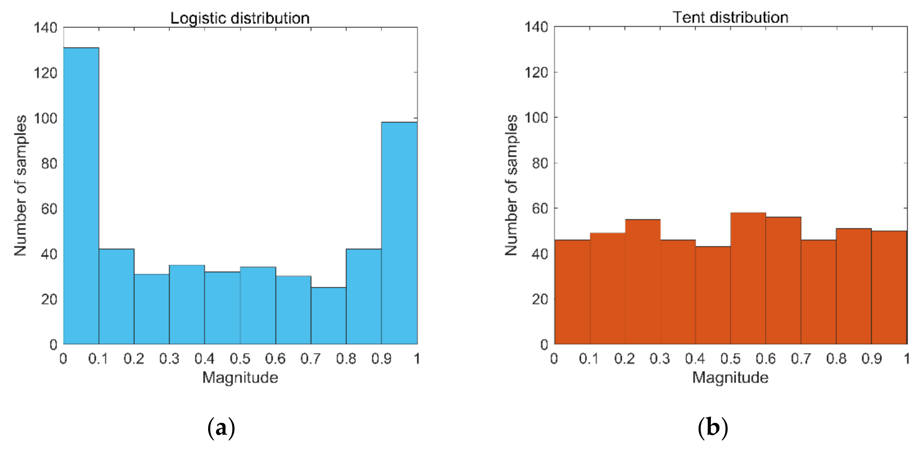
• Tent chaotic map helps the IHSSAO to increase the original population diversity.
• PIOBL helps the proposed algorithm to increase the original population diversity and the capability to escape from local optima.
• To verify the performance of the proposed IHSSAO, we tested it against the SSA, AO, and five other advanced meta-heuristic algorithms by 23 classical benchmark functions and 17 IEEE CEC2017 test functions.
• Eventually, we applied the IHSSAO, SSA, and AO to the UAV path planning problem. The experimental results verify that the proposed IHSSAO is superior to the basic SSA and AO in solving the path planning problem for UAVs in complex terrain.

The rest of this paper is organized as follows. Section 2 presents the background knowledge of basic SSA and AO, as well as tent chaotic map and pinhole imaging opposition-based learning strategies. Section 3 provides a detailed description of the proposed IHSSAO. In Section 4, a series of simulation experiments are conducted to evaluate the performance of IHSSAO, and the obtained results are discussed. Based on this, the proposed method in Section 5 is applied to solve the UAV path planning in complex terrain. Finally, Section 6 shows the conclusions and future research directions of this paper.

2. Preliminary Knowledge

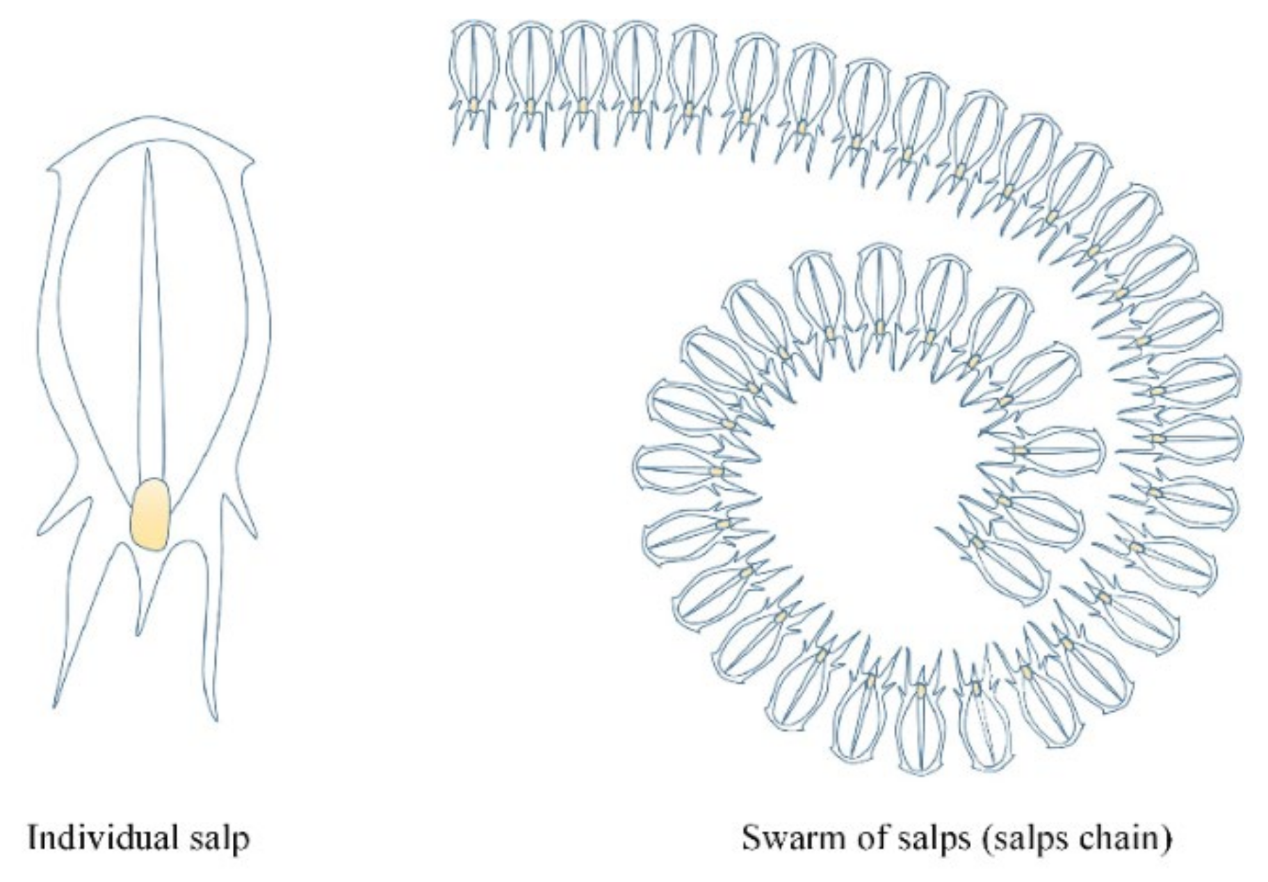
2.1. Salp Swarm Algorithm

The SSA is a new bio-inspired optimization algorithm proposed by Mirjalili et al. [16] which simulates the group behavior of bottle sea squirts while navigating and foraging in the ocean. In Figure 1, the slap propels itself by inhaling and expelling seawater, preying on phytoplankton in the water. During the feeding process, individuals in the slap swarm are connected to each other and form long chains in a circular pattern. In SSA, the slap chain is composed of two types of slap swarm: leaders and followers. The leader is at the front of the slap chain to lead the whole swarm, while the other individuals play the role of followers. During the foraging process, the whole population moves gradually towards the food position in this way.

In SSA, the position vector $X$ of each salp individual is defined for searching in the $N$ dimensional space, where $N$ is the number of decision variables. The position vector $X$ will consist of $N$ salp individuals in the $D$ dimensions, so the population vector consists of $N\times D$ dimensional matrix, i.e.,

$$X=\left[\begin{array}{ccc}{x}_{1,1}& \dots & x_{1,D}\\ ⋮& \ddots & ⋮\\ x_{N,1}& \dots & x_{N,D}\end{array}\right]$$

(1)

The location of the food source is the target location for the whole swarm of salp, hence the leader’s position update formula is as follows:

$$X_{i,j}=l{b}_j+rand\times \left(u{b}_j-l{b}_j\right)$$

(2)

$$X_{1,j}(t+1)=\{\begin{array}{l}{F}_j(t)+c_1\left(\left(u{b}_j-l{b}_j\right)c_2+l{b}_j\right),c_3\ge 0.5\hfill \\ F_j(t)-c_1\left(\left(u{b}_j-l{b}_j\right)c_2+l{b}_j\right),c_3<0.5\hfill \end{array}$$

(3)

where $X_{1,j}\left(t+1\right)$ represents the position of the leader in the $j\mathrm{th}$ dimension; $F_j\left(t\right)$ shows the location of the food source in the $j\mathrm{th}$; $u{b}_j$ and $l{b}_j$ denote the upper and lower bounds of the $j$th dimensional space, respectively; $c_1$, $c_2,$ and $c_3$ are the random numbers. The parameters $c_2$ and $c_3$, which are random numbers uniformly generated in the interval of $\left[0,1\right],$ determine whether the next position in the $j$th dimension should be in the positive or negative direction and the length of the move. In SSA, the parameter $c_1$ is the most important parameter, which can make the exploration ability of the algorithm in a better state.

$$c_1=2e^{-{\left(4t/T\right)}^2}$$

(4)

where $t$ is the current iteration number and $T$ is the maximum iteration number.

When the position of the first salp is updated, the other individuals in the salp swarm follow to move. The mathematical model of this behavior is as follows:

$$X_{i,j}(t+1)=\frac{1}{2}\left(X_{i,j}(t)+X_{i-1,j}(t)\right)$$

(5)

where $x_{i,j}\left(t+1\right)$ shows the position of $i$th follower salp in $j$th dimension.

2.2. Aquila Optimizer

Aquila Optimizer proposed by Abualigah et al. in 2021 is a novel meta-heuristic optimization algorithm. The Aquila has four types of hunting behavior for various species of prey. Aquila can flexibly switch its hunting strategies for different prey species before it attacks the prey using its rapid speed and its sturdy feet and claws. The mathematical model is briefly described as follows [23].

2.2.1. Expanded Exploration ($X_1$)

In this phase, Aquila identifies prey areas and selects the best areas to hunt by soaring high in a vertical dive. Aquila Optimizer explores extensively from high altitude soaring to ascertain the range of search space in which prey is located. The mathematical expression of this behavior is as follows:

$$X_1(t+1)=X_{best}(t)\times (1-\frac{t}{T})+\left(X_M(t)-X_{best}(t)\times rand\right)$$

(6)

$$X_M(t)=\frac{1}{N}{\displaystyle \sum _{i=1}^N{X}_i(t)}$$

(7)

where $X_1\left(t+1\right)$ is the position of the $t+1$ iteration generated by the expanded exploration. $X_{best}\left(t\right)$ shows the best-obtained solution thus far, which can reflect the approximate position of prey. $X_M\left(t\right)$ represents the average solution at the tth iteration. $rand$ is a random value between $0$ and $1$. $t$ and $T$ denote the current number of iterations and the maximum iterations, respectively. $N$ is the number of the population.

2.2.2. Narrowed Exploration ($X_2$)

When the area of prey is spotted at a high altitude, the Aquila hovers above the target prey, prepares to land, and then attacks. In preparation for the attack, Aquila carefully explores a specific area for prey. This behavior is expressed mathematically as follows.

$$X_2(t+1)=X_{best}(t)\times Levy(D)+X_R(t)+(y-x)\times rand$$

(8)

where $D$ is the dimension size, $Levy\left(D\right)$ is the Levy flight distribution function calculated by Equation (9), $X_R\left(t\right)$ denotes a random solution within $\left[1,N\right]$ during the ith iteration.

$$Levy(D)=s\times \frac{u\times \sigma }{|v{|}^{1/\beta }}$$

(9)

$$\sigma =\left(\frac{\Gamma (1+\beta )\times \sin (\frac{\pi \beta }{2})}{\Gamma (\frac{1+\beta }{2})\times \beta \times 2^{(\frac{\beta -1}{2})}}\right)$$

(10)

where $s$ and $\beta$ are, respectively, constant values equal to $0.01$ and $1.5$, $u$ and $v$ are random values within the interval of $\left[0,1\right]$, and $y$ and $x$ are calculated for rendering the spirals in the search as follows.

$$y=r\times \cos (\theta )$$

(11)

$$x=r\times \sin (\theta )$$

(12)

$$r=r_1+U\times D_1$$

(13)

$$\theta =-\omega \times D_1+{\theta }_1,{\theta }_1=\frac{3\times \pi }{2}$$

(14)

where $r_1$ represents the number of search cycles, which has a value from $1$ to $20$, $D_1$ is composed of integer numbers from $1$ to the dimension size $\left(D\right)$, $U$ is a fixed value of $0.00565,$ and $\omega$ is a fixed value of $0.005$.

2.2.3. Expanded Exploitation ($X_3$)

In the third method, the prey area is accurately assigned and the Aquila is prepared for landing and attacking. Aquila descends vertically and makes the initial attack to observe the prey’s reaction. This method is known as a low-altitude slow descent attack. Here, the Aquila approaches the prey using a target area and performs the attack. This behavior is mathematically represented as follows.

$$X_3(t+1)=\left(X_{best}(t)-X_M(t)\right)\times \alpha -rand+((ub-lb)\times rand+lb)\times \delta$$

(15)

where $X_{best}\left(t\right)$ denotes to the best position obtained so far and $X_M\left(t\right)$ means the average value of the current positions. The exploitation adjustment parameters $\alpha$ and $\delta$ are fixed in this paper at $0.1$, $rand$ is a random value between $0$ and $1$, and $ub$ and $lb$ are the upper and lower boundaries of the given problem.

2.2.4. Narrowed Exploitation ($X_4$)

When Aquila approaches the prey, it attacks the prey on land according to its random movements. Definitively, Aquila attacks the prey in the last position. This behavior can be expressed mathematically as follows.

$$X_4(t+1)=QF\times X_{best}(t)-\left(G_1\times X(t)\times rand\right)-G_2\times Levy(D)+rand\times G_1$$

(16)

$$QF(t)=t^{\frac{2\times r_8-1}{{(1-T)}^2}}$$

(17)

$$G_1=2\times rand-1$$

(18)

$$G_2=2\times (1-\frac{t}{T})$$

(19)

where $X\left(t\right)$ is the current position. $QF\left(t\right)$ represents the quality function value, which is used to balance the search strategy. $G_1$ denotes the movement parameter of Aquila whilst tracking the prey, which is a random number between $\left[-1,1\right]$. $G_2$ denotes the flight slope when chasing the prey, which decreases linearly from $2$ to $0$. $rand$ is a random number between $0$ and $1$.

2.3. Tent Chaotic Map

Tent chaotic map has the characteristic of randomness, ergodicity, and orderliness. Attributed to its distinctive features many scholars have introduced tent chaotic map into the Whale Optimization Algorithm [28], Antlion Optimizer Algorithm [29], COOT Bird Algorithm [30], and other heuristic optimization algorithms in recent years, which can greatly increase the diversity of the population and accelerate the convergence speed of the algorithm in the early stage. In this paper, we select the tent chaotic map to replace the original method of random population initialization to enhance the population diversity of the proposed IHSSAO with the following equation.

$$z_{k+1}=\left\{\begin{array}{ll}2z_k,& 0\le z_k<0.5\\ 2(1-z_k),& 0.5\le z_k\le 1\end{array}\right.$$

(20)

The formula transformed from Equation (20) by Bernoulli shift is

$$z_{k+1}=(2z_k)\mathrm{mod}1$$

(21)

The specific steps of using the tent chaotic map to generate sequence values are listed below.

Step 1:

Randomly generate $z_0$ between the intervals $\left(0,1\right)$ (avoiding $z_0$ in small periods $\left(0.2,0.4,0.6,0.8\right)$, $y\left(1\right)=z_0$, $i=j=1$.

Step 2:

Iterate through Equation (21) to obtain a sequence of $z_i$, $i=i+1$.

Step 3:

If the maximum number of iterations is reached, then turn to Step 4. Otherwise, if $z_i=\left\{0,0.25,0.5,0.75\right\}$ or $x_i=x_i-k, k=\left\{0,1,2,3,4\right\}$, change the initial value of the iteration by the equation $x\left(i\right)=y\left(j+1\right)=y\left(j\right)+c,$ where $c$ is a random number, $j=j+1$. Otherwise return Step 2.

Step 4:

The operation is halted and the $x$ sequence is retained.

Figure 2a,b represent the distribution histogram of the tent chaotic map and logistic chaotic map in the interval $\left[0,1\right]$ with the initial value of 0.32 and the iteration times of 500, respectively. The experimental results indicate that the sequence generated by tent chaos map has significantly better uniformity than the logistic chaos sequence. Therefore, we utilize the tent chaotic map to initialize the positions of search agents, which can not only enhance the search capability of the algorithm, but also reduce the influence of initial values on the optimization performance.

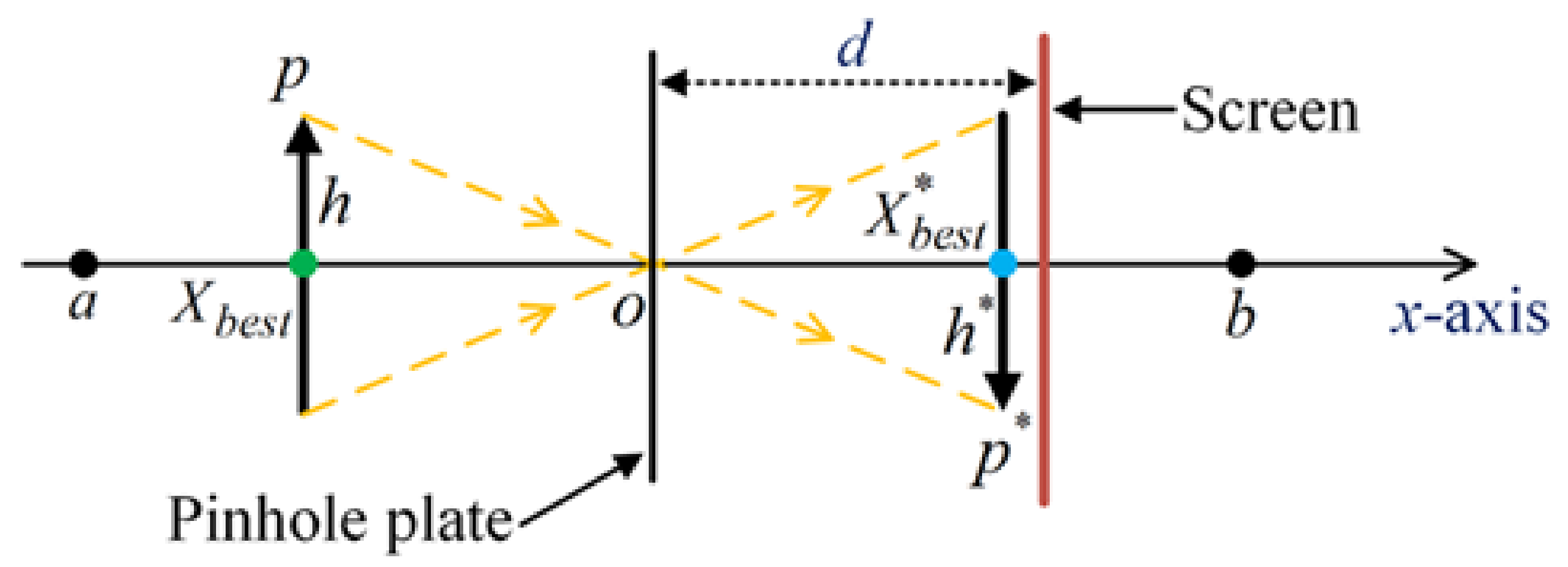
2.4. Pinhole Imaging Opposition-Based Learning

To help the algorithm get rid of the local optima, some scholars have tried to combine opposition-based learning (OBL) [31,32] with intelligent optimization algorithms to expand the search range by calculating the reverse solution of the current feasible solution, and thus find out the candidate solutions at more optimal positions. Based on this idea, Zhang et al. [33] successfully used the pinhole imaging opposition-based learning to improve the convergence accuracy and speed of the modified Whale Optimization Algorithm. In this paper, we attempt to introduce this strategy to increase the possibility of the IHSSAO jumping out of the local optima. The basic schematic of PIOBL is shown in Figure 3.

In the figure, the upper and lower boundaries of the coordinate axes are $a,b$. There is a small aperture screen placed at the base point $O$. $X_{best}$ (the current global optimal solution) represents the projection of the light source $P$ whose height is $h$ on the x-axis, when the light source through the small aperture will get an inverted image $p^{*}$ of height $h^{*}$ at the imaging screen, at which time the projection of $p^{\prime }$ on the x-axis is $X_{best}^{*}$ (the newly generated inverse solution). According to the geometric relationship of the line segments in the figure, it can be derived that:

$$\frac{(a+b)/2-X_{best}}{X_{best}^{*}-(a+b)/2}=\frac{h}{h^{*}}$$

(22)

Let $h/h^{*}=K$ be substituted into the above equation, and the variation yields the expression for $X_{best}^{*}$:

$$X_{best}^{*}=\frac{(a+b)}{2}+\frac{(a+b)}{2K}-\frac{X_{best}}{K}$$

(23)

When the algorithm is solving a high-dimensional complex function, the small-aperture inverse learning solution can be computed by the following equation:

$$X_{best,j}^{*}=(a_j+b_j)/2+(a_j+b_j)/2K-X_{best,j}/K$$

(24)

where $X_{best,j}$ is the optimal solution in the $j\mathrm{th}$ dimension, $X_{best,j}^{*}$ denotes the inverse solution of $X_{best,j}$, respectively, and $a_j$ and $b_j$ are the minimum and maximum values in the $jth$ dimension on the search space.

When $K=1$, Equation (25) can be simplified as follows:

$$X_{best}^{*}=a+b-X_{best}$$

(25)

It can be seen that when $K=1$ the PIOBL is the common OBL strategy. The candidate solutions obtained by the common OBL strategy are generally fixed, but a wider range of inversion positions can be obtained by changing the distance between the imaging screen and the pinhole plate to adjust the scale factor $K$ in the PIOBL strategy.

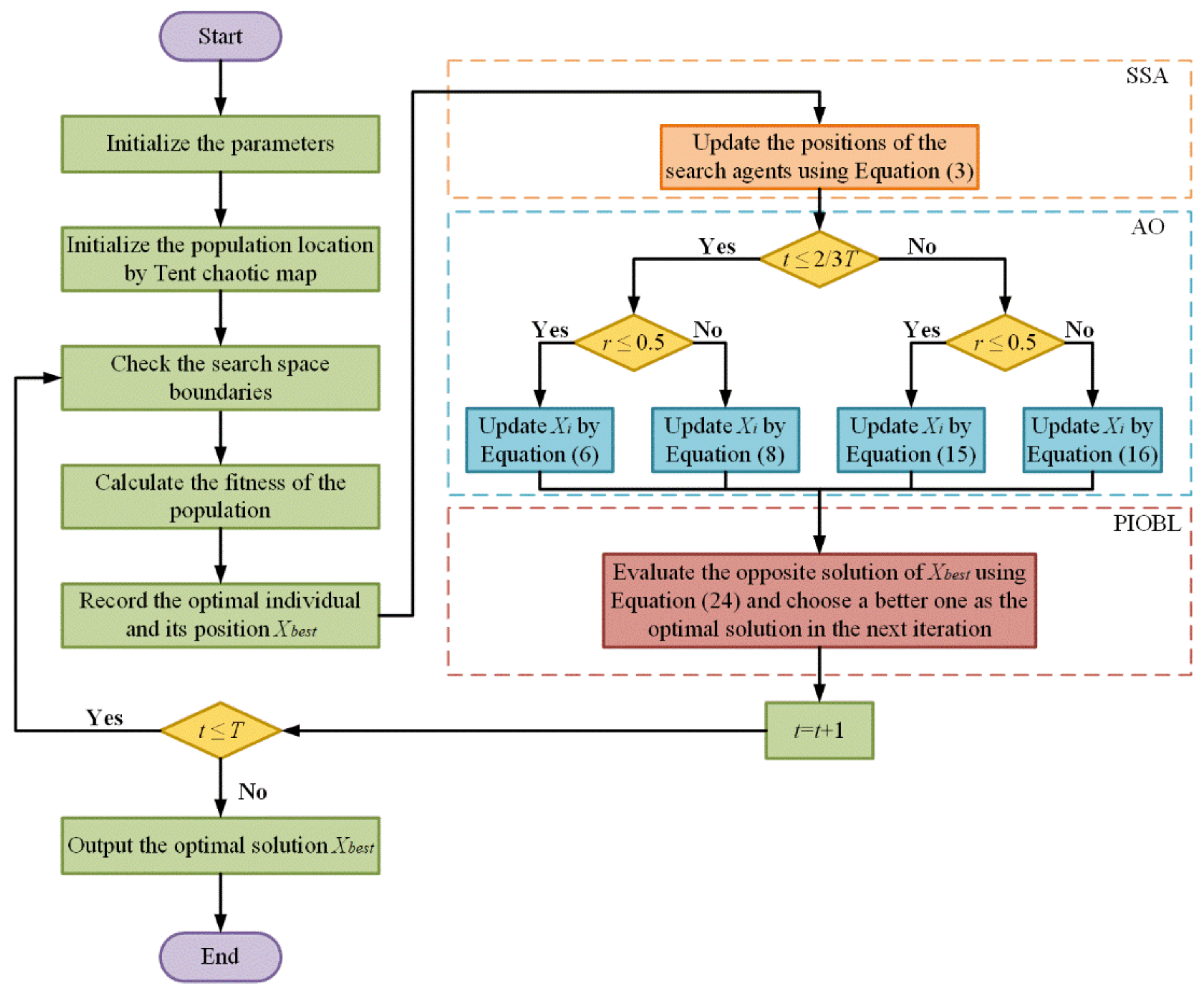
3. The Proposed Algorithm

In this section, we describe the flow of the proposed IHSSAO algorithm in detail. Our proposed algorithm is mainly based on AO and is enhanced with the leadership mechanism of SSA, tent chaotic map, and PIOBL strategy. In the initial stage, we use the tent chaotic map to generate the initial population, thus promoting the population diversity. After that, the following process is iteratively executed. Firstly, before the AO algorithm is executed, we update the population position by the leader mechanism of SSA, i.e., Equation (2). The introduction of the SSA leader mechanism in the proposed algorithm effectively enhances the exploitation capability of the original AO. Secondly, the position update formulas of the different four stages of AO are executed using Equation (6), Equation (8), Equation (15), or Equation (16), depending on the specific situation. Finally, the optimal position $X_{best}$ and the fitness value are filtered out using Equation (24) from the PIOBL strategy. The PIOBL strategy enhances the ability to escape from the local optimum. After completing the last iteration, the optimal value $X_{best}$ is output. The flow chart and pseudo-code of the proposed IHSSAO are shown in Figure 4 and Algorithm 1, respectively.

Algorithm 1 Pseudo-code of the proposed IHSSAO algorithm

1. Input the population $N$, and the generation number $T$

2. Initialize the positions of each individual by tent chaotic map $X_i\left(i=1,2,\cdots ,N\right)$//tent chaotic map

3. While $t\le T$

4.  Check if the position goes beyond the search space boundary and then adjust it

5.  Evaluate the fitness values of all search agents

6.  Update the global optimum $X_{best}$

7.  $\mathrm{Calculate} X_i$ using Equation (3)    //SSA

8.  For $i=1$ to $N$

9.    If t ≤ $\frac{2}{3}$T then    //AO

10.    If $r\le 0.5$ then

11.     Update the position using Equation (6)

12.    Else

13.     Update the position using Equation (8)

14.    End if

15.   Else

16.    If $r\le 0.5$ then

17.     Update the position using Equation (15)

18.    Else

19.     Update the position using Equation (16)

20.    End if

21.   End if

22.  End For

23.  Generate the opposite position of $X_{best}$ using Equation (24) and save the one with better fitness    //PIOBL

24.  $t=t+1$

25. End While

26. Return $X_{best}$

4. Experimental Results and Discussion of IHSSAO Performance Verification

In this section, the performance of the IHSSAO in solving numerical optimization problems is examined by selecting 23 classical benchmark functions and 17 CEC2017 benchmark functions for comparison experiments with other meta-heuristic algorithms. All simulation experiments are conducted in MATLAB R2017a in Microsoft Windows 10 with a computer hardware platform configuration of Intel^® Core^TM i7-9750H @ 2.60 GH and RAM 8 G.

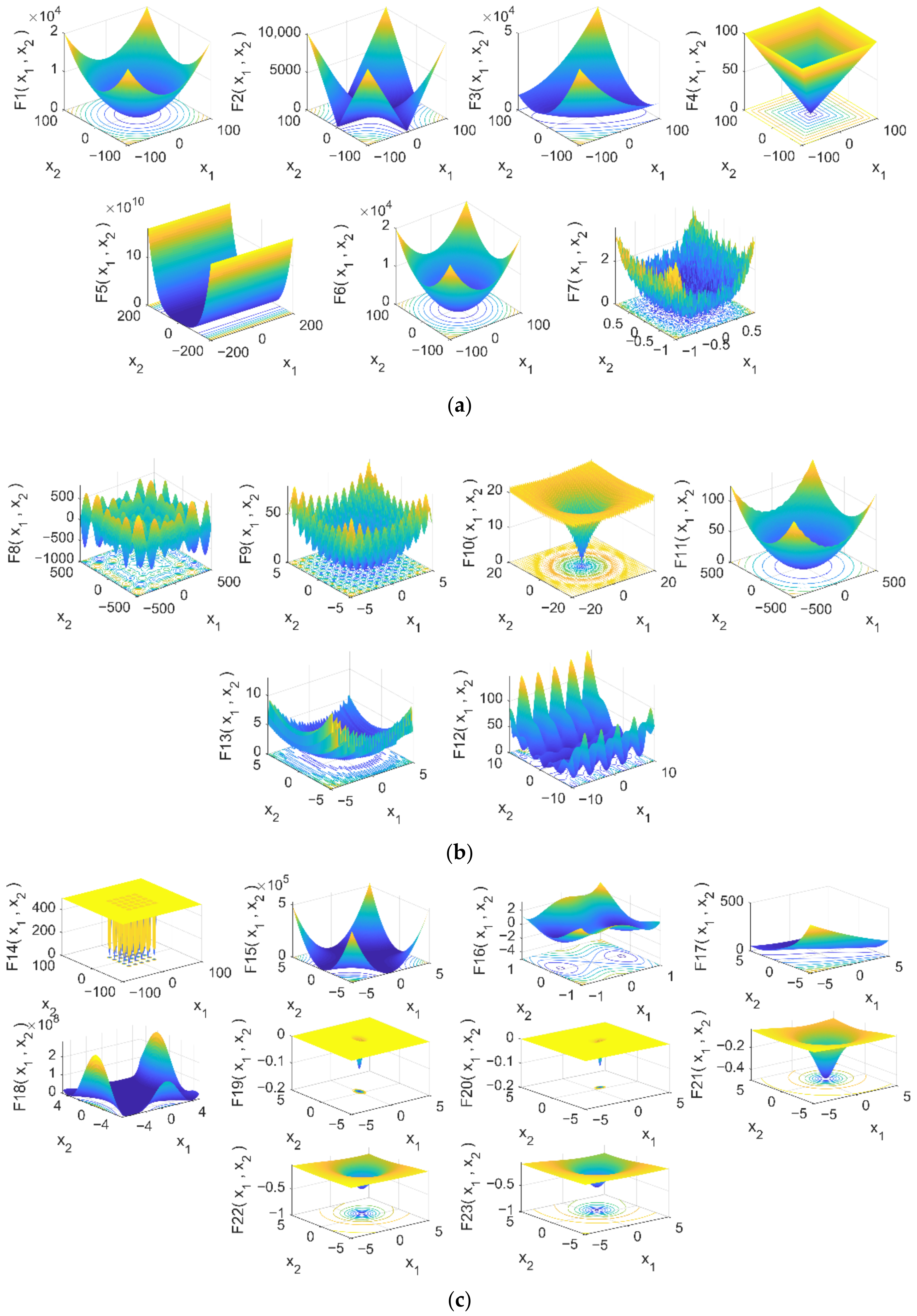
4.1. Experiment I: Classical Benchmark Function

In this study, there are three various categories including unimodal (UM), multimodal (MM), and fix-dimension multimodal (FM) in the 23 benchmark functions. Among them, the UM functions ($F_1$–$F_7$) including only one global minimum are often selected to test the local exploitation and convergence rate ability of the algorithm. $F_8$–$F_{13}$ are MM functions containing multiple locally optimal solutions in the search space, and their number grows exponentially as the number of dimensions increases. It is well suited to evaluate the ability of the algorithm to explore and avoid getting trapped in local optima. The FM functions ($F_{14}$–$F_{23}$) used to evaluate the stability of the algorithm are a combination of the UM function and MM function, but with lower dimensionality.

Table 1. Unimodal benchmark function.

Function	Name	Dim	Range	Fmin
$F_1(x)={\displaystyle \sum _{i=1}^D}{x}_i^2$	Sphere	30	[−100, 100]	0
$F_2(x)={\displaystyle \sum _{i=1}^D}|x_{\mathrm{i}}|+{\displaystyle \prod _{i=1}^D}|x_{\mathrm{i}}|$	Schwefel 2.22	30	[−10, 10]	0
$F_3(x)={\displaystyle \sum _{i=1}^D}{({\displaystyle \sum _{j=1}^D}{x}_j)}^2$	Schwefel 1.2	30	[−100, 100]	0
$F_4(x)={\max }_i\left\{\left|x_i\right|,1\le i\le D\right\}$	Schwefel 2.21	30	[−100, 100]	0
$F_5(x)={\displaystyle \sum _{i=1}^{D-1}}[100{(x_{i+1}-x_i^2)}^2+{(x_i-1)}^2]$	Rosenbrock	30	[−30, 30]	0
$F_6(x)={\displaystyle \sum _{i=1}^D}{\left(\left|x_i+0.5\right|\right)}^2$	Step	30	[−100, 100]	0
$F_7(x)={\displaystyle \sum _{i=1}^D}i{x}_i^4+random[0,1)$	Quartic	30	[−1.28, 1.28]	0

,

Table 2. Multimodal benchmark function.

Function	Name	Dim	Range	Fmin
$F_8(x)={\displaystyle \sum _{i=1}^D}-x_i\sin \left(\sqrt{\left|x_i\right|}\right)$	Schwefel 2.26	30	[−500, 500]	−418.9829 × Dim
$F_9(x)={\displaystyle \sum _{i=1}^D}[x_i^2-10\cos \left(2\pi x_i\right)+10]$	Rastrigin	30	[−5.12, 5.12]	0
$\begin{array}{l}{F}_{10}(x)=-20\exp (-0.2\sqrt{\frac{1}{n}{\displaystyle \sum _{i=1}^D}{x}_i^2})-\\ \exp (\frac{1}{n}{\displaystyle \sum _{i=1}^D}\cos (2\pi x_i))+20+e\end{array}$	Ackley	30	[−32, 32]	0
$F_{11}(x)=\frac{1}{4000}{\displaystyle \sum _{i=1}^D}{x}_i^2-{\displaystyle \prod _{i=1}^D}\cos (\frac{x_i}{\sqrt{i}})+1$	Griewank	30	[−600, 600]	0
$\begin{array}{l}{F}_{12}(x)=\frac{\pi }{D}\{10\sin (\pi y_1)+{\displaystyle \sum _{i=1}^{D-1}}{(y_i-1)}^2[1+10{\sin }^2(\pi y_{i+1})]+\\ {(y_n-1)}^2\}+{\displaystyle \sum _{i=1}^D}u\left(x_i,10,100,4\right)\\ y_i=1+\frac{x_i+1}{4},u\left(x_i,a,k,m\right)=\left\{\begin{array}{l}k{\left(x_i-a\right)}^m{x}_i>a\\ 0-a<x_i<a\\ k{\left(-x_i-a\right)}^m{x}_i<-a\end{array}\right.\end{array}$	Penalized	30	[−50, 50]	0
$\begin{array}{l}{F}_{13}(x)=0.1\{{\sin }^2(3\pi x_i)+{\displaystyle \sum _{i=1}^D}{(x_i-1)}^2[1+{\sin }^2(3\pi x_i+1)]+\\ {(x_D-1)}^2[1+{\sin }^2(2\pi x_D)]\}+{\displaystyle \sum _{i=1}^D}u\left(x_i,5,100,4\right)\end{array}$	Penalized2	30	[−50, 50]	0

and

Table 3. Fix-dimension multimodal benchmark function.

Function	Name	Dim	Range	Fmin
$\begin{array}{c}\hfill F_{14}\left(x\right)=(\frac{1}{500}+{\displaystyle \sum _{j=1}^{25}}(j+\underset{i=1}{\sum ^n}{(x_i-a_{ij})}^6{)}^{-1}{)}^{-1}\end{array}$	Foxholes	2	[−65, 65]	0.998
$\begin{array}{c}\hfill F_{15}\left(x\right)={\displaystyle \sum _{i=1}^{11}}[a_i-\frac{x_1(b_i^2+b_i{x}_2)}{b_i^2+b_i{x}_3+x_4}]{}^2\end{array}$	Kowalik	4	[−5, 5]	0.00030
$F_{16}(x)=4x_1^2-2.1x_1^4+\frac{1}{3}{x}_1^6+x_1{x}_2-4x_2^2+4x_2^4$	Six-hump Camel Back	2	[−5, 5]	−1.0316
$F_{17}(x)={(x_2-\frac{5.1}{4{\pi }^2}{x}_1^2+\frac{5}{\pi }{x}_1-6)}^2+10(1-\frac{1}{8\pi })\cos x_1+10$	Branin	2	[−5, 5]	0.398
$\begin{array}{l}{F}_{18}(x)=\left[1+{\left(x_1+x_2+1\right)}^2\left(19-14x_1+3x_1^2-14x_2+6x_1{x}_2+3x_2^2\right)\right]\\ \times \left[30+{\left(2x_1-3x_2\right)}^2\times \left(18-32x_2+12x_1^2+48x_2-36x_1{x}_2+27x_2^2\right)\right]\end{array}$	Goldstein Price	2	[−2, 2]	3
$F_{19}(x)=-{\displaystyle \sum _{i=1}^4}{c}_i\exp (-{\displaystyle \sum _{j=1}^3}{a}_{ij}{(x_j-p_{ij})}^2)$	Hartman 3	3	[−1, 2]	−3.8628
$F_{20}(x)=-{\displaystyle \sum _{i=1}^4}{c}_i\exp (-{\displaystyle \sum _{j=1}^6}{a}_{ij}{(x_j-p_{ij})}^2)$	Hartman 6	6	[0, 1]	−3.32
$F_{21}(x)=-{\displaystyle \sum _{i=1}^5}{[(X-a_i){(X-a_i)}^T+c_i]}^{-1}$	Langermann 5	4	[0, 10]	−10.1532
$F_{22}(x)=-{\displaystyle \sum _{i=1}^7}{[(X-a_i){(X-a_i)}^T+c_i]}^{-1}$	Langermann 7	4	[0, 10]	−10.4028
$F_{23}(x)=-{\displaystyle \sum _{i=1}^{10}}{[(X-a_i){(X-a_i)}^T+c_i]}^{-1}$	Langermann 10	4	[0, 10]	−10.5363

show the expressions, dimensions, search ranges, and theoretical optima of these benchmark functions, respectively. In addition, Figure 5 shows the 3D view of the search space for 23 benchmark functions.

4.1.1. Parameter Setting

To validate the performance of the modified algorithm, the IHSSAO algorithm was compared with the original SSA, AO, and five advanced meta-heuristics, i.e., WOA, HHO, Multi-Verse Optimizer (MVO), Sooty Tern Optimization Algorithm (STOA), and Tunicate Swarm Algorithm (TSA). For all these algorithms, the population size and the maximum number of iterations are set as 30 and 500, respectively. We ran each algorithm independently for 30 times according to the parameter settings as shown in

Table 4. Parameter settings for the optimization algorithms.

Algorithm	Parameters
WOA [13]	$b=1; a_1=\left[2, 0\right]; a_2=\left[-1,-2\right]$
HHO [14]	$\beta =1.5; E_0\in \left[-1, 1\right]$
SSA [16]	$c_1=\left[1, 0\right]; c_2,c_3\in \left[0, 1\right]$
MVO [34]	$WEP\in \left[0.2, 1\right]; TDR\in \left[0, 1\right]; r_1,r_2,r_3\in \left[0, 1\right]$
STOA [35]	$C_f=2; C_b\in \left[0, 0.5\right]; u,v=1$
TSA [36]	$P_{max}=4, P_{min}=1$
AO [23]	$U=0.00565; r_3=10; \alpha =0.1; \delta =0.1; \omega =0.005; G_1\in \left[-1, 1\right]; G_2=\left[2, 0\right]$

.

4.1.2. Assessment Standards of Performance

In this section, we introduce two metrics for evaluating the algorithm performance, namely, the average fitness value (Avg) and standard deviation (Std). The Avg visually characterizes the convergence effectiveness and search capability of the algorithm. Additionally, the Std indicates the degree of deviation of the experimental results from the mean. The expressions of Avg and Std are as follows, respectively.

$$\mathrm{Avg}=\frac{1}{n}{\displaystyle \sum _{k=1}^n{S}_k}$$

(26)

$$\mathrm{Std}=\sqrt{\frac{1}{n-1}{\displaystyle \sum _{k=1}^n{\left(S_k-\mathrm{Avg}\right)}^2}}$$

(27)

where $n$ denotes the number of times the algorithm has been run and $S_k$ is the result obtained after each execution.

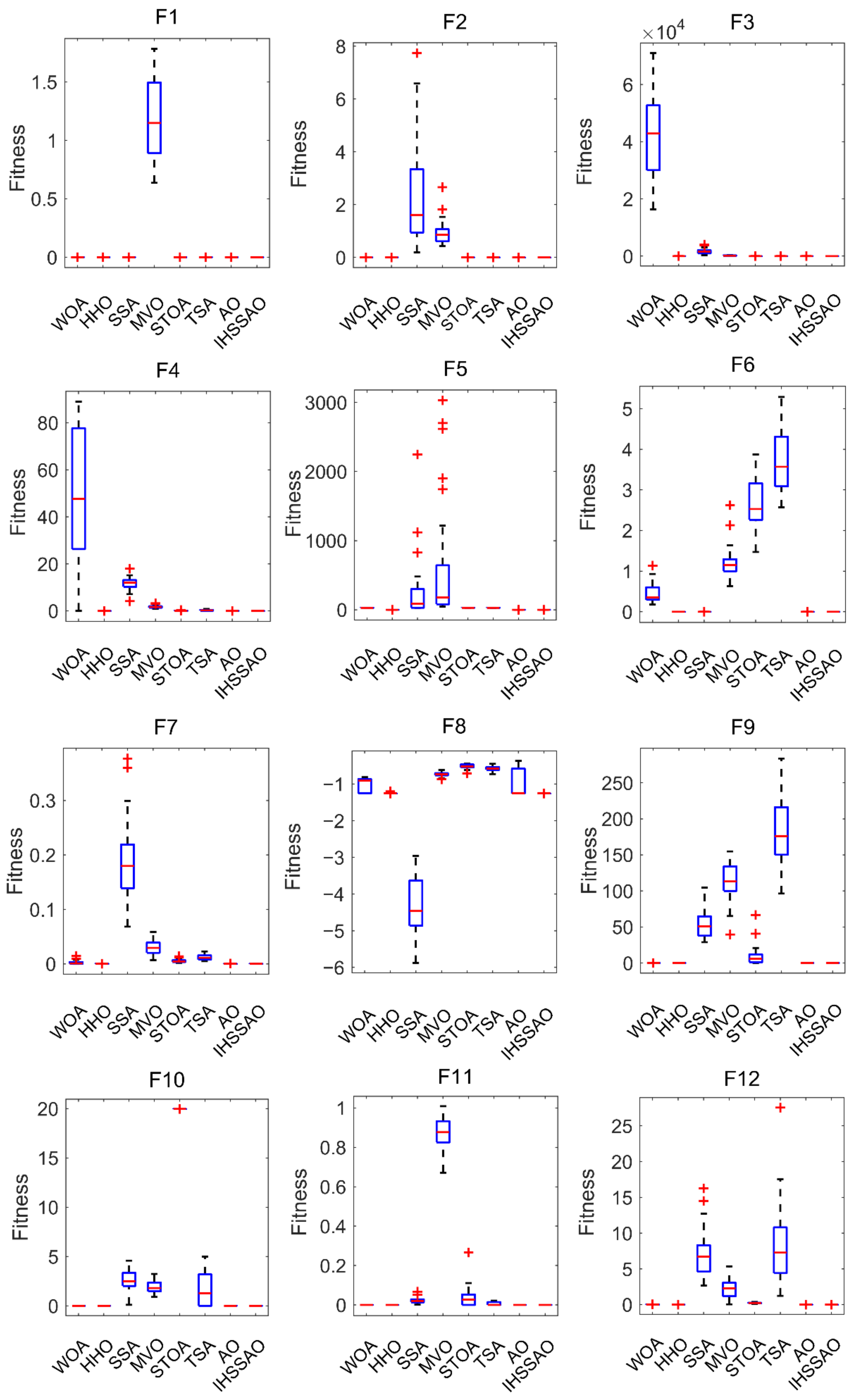
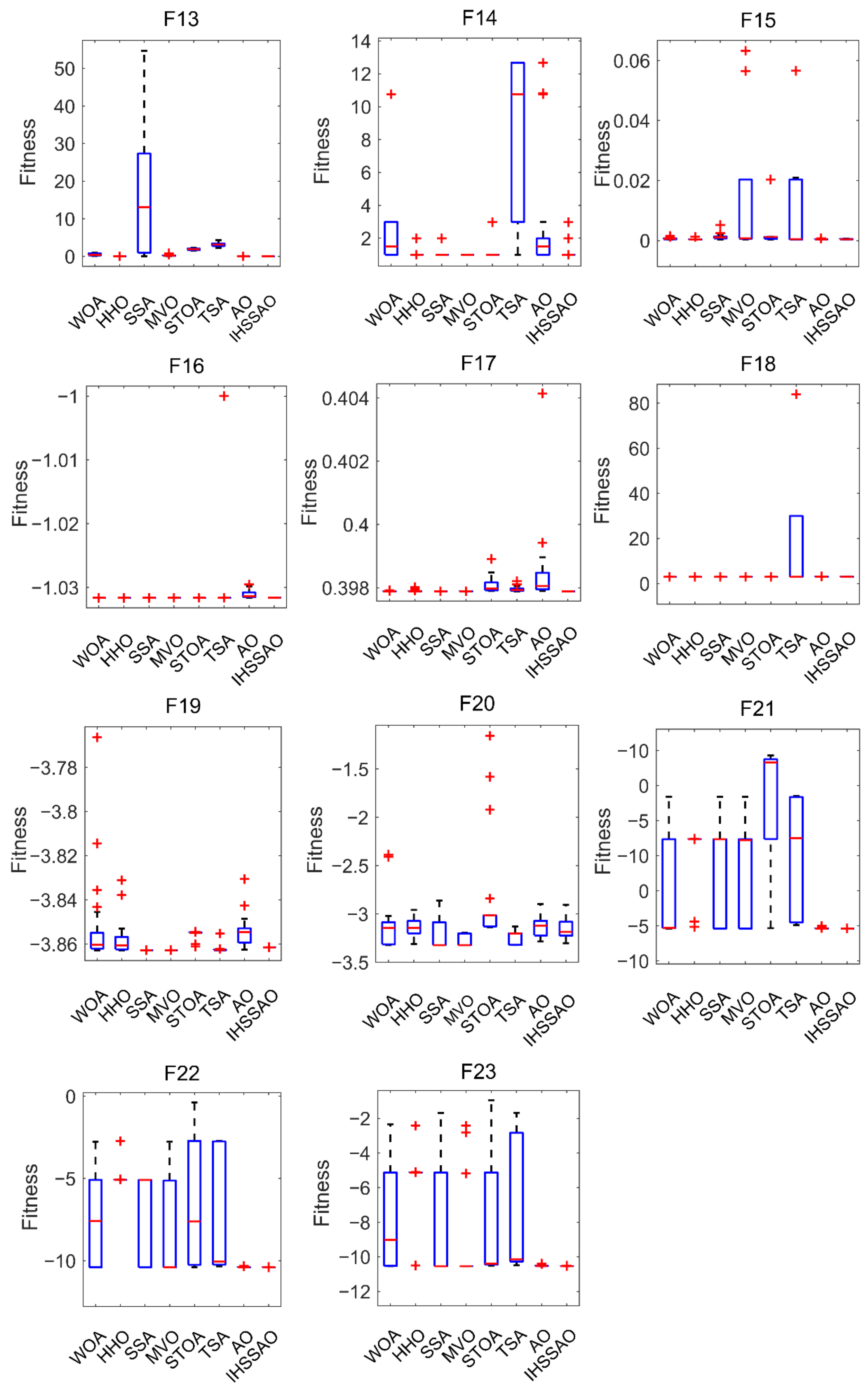
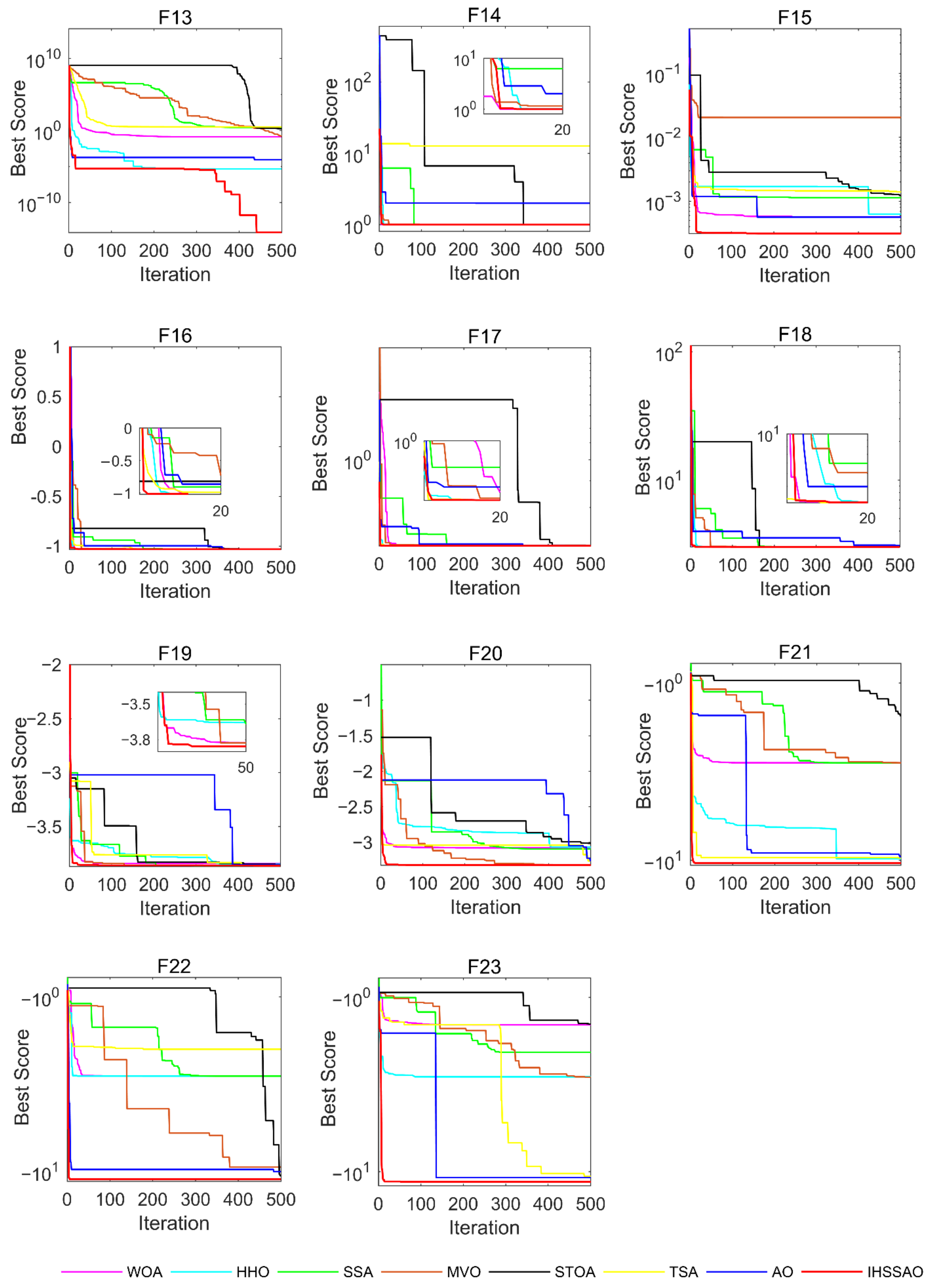
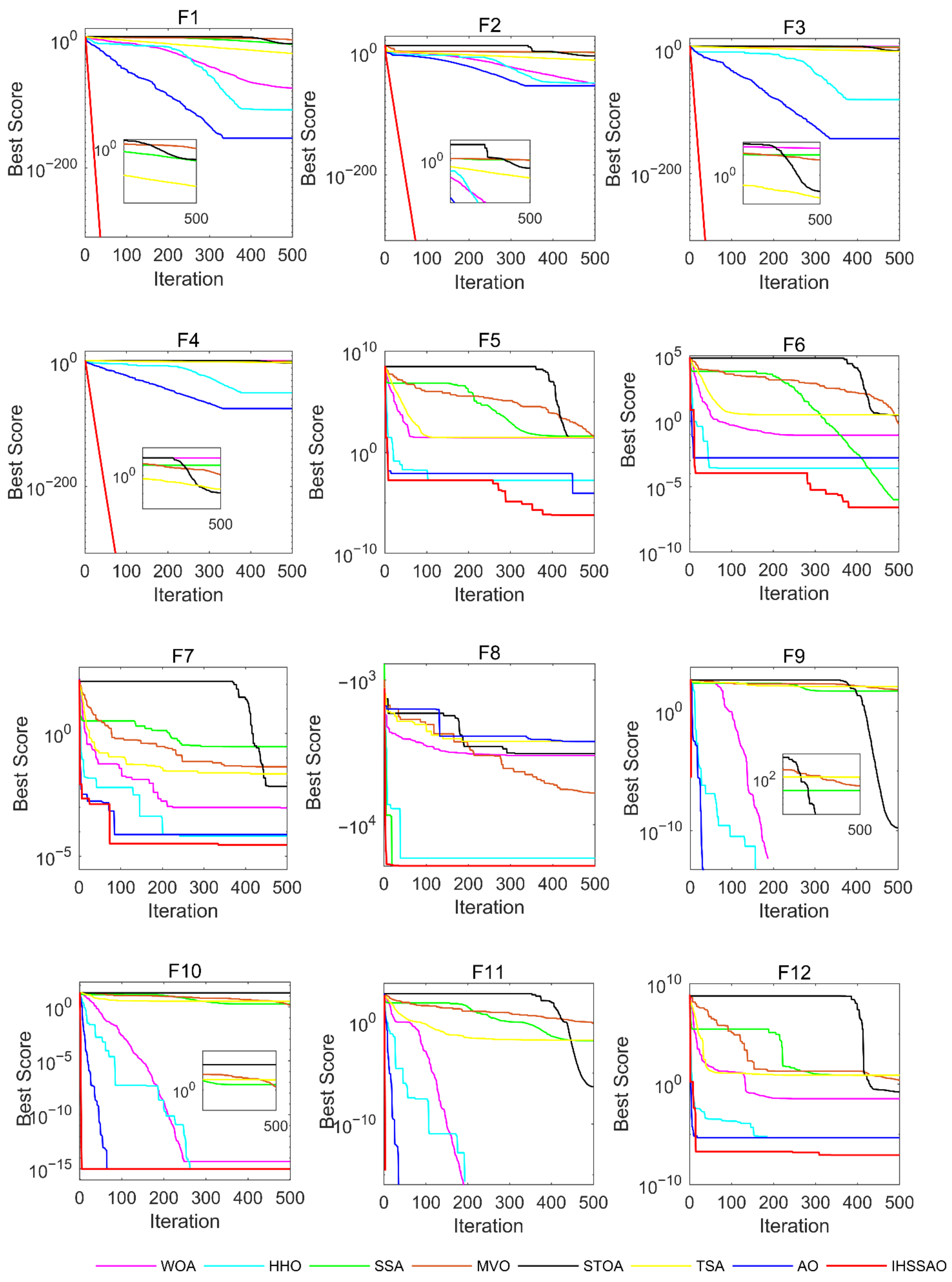
4.1.3. Comparison with IHSSAO and Other Algorithms

The Avg and Std obtained by the IHSSAO after running in 23 benchmark functions are shown in

Table 5. Comparison results of various algorithms on 23 benchmark functions.

${\mathit{F}}_{\mathit{n}}$	Metric	WOA	HHO	SSA	MVO	STOA	TSA	AO	IHSSAO
$F_1$	Avg	3.07 × 10−72	3.72 × 10−94	1.53 × 10−7	1.17 × 100	8.28 × 10−7	2.46 × 10−21	1.56 × 10−104	0.00 × 100
	Std	1.37 × 10−71	1.84 × 10−93	1.29 × 10−7	3.35 × 10−1	1.41 × 10−6	5.54 × 10−21	8.52 × 10−104	0.00 × 100
$F_2$	Avg	2.06 × 10−51	3.17 × 10−50	2.32 × 100	9.27 × 10−1	7.97 × 10−6	1.06 × 10−13	8.53 × 10−57	0.00 × 100
	Std	8.00 × 10−51	9.82 × 10−50	1.95 × 100	4.70 × 10−1	6.96 × 10−6	1.29 × 10−13	3.76 × 10−56	0.00 × 100
$F_3$	Avg	4.24 × 104	1.07 × 10−76	1.72 × 103	1.92 × 102	8.82 × 10−2	8.91 × 10−5	1.58 × 10−101	0.00 × 100
	Std	1.51 × 104	5.82 × 10−76	9.89 × 102	6.60 × 101	1.57 × 10−1	2.42 × 10−4	8.63 × 10−101	0.00 × 100
$F_4$	Avg	4.89 × 101	3.43 × 10−47	1.15 × 101	1.81 × 100	6.38 × 10−2	2.70 × 10−1	9.68 × 10−54	0.00 × 100
	Std	2.95 × 101	1.87 × 10−46	2.81 × 100	6.14 × 10−1	8.84 × 10−2	2.29 × 10−1	3.16 × 10−53	0.00 × 100
$F_5$	Avg	2.80 × 101	1.02 × 10−2	2.76 × 102	6.11 × 102	2.84 × 101	2.81 × 101	5.80 × 10−3	2.49 × 10−5
	Std	5.37 × 10−1	1.14 × 10−2	4.50 × 102	8.88 × 102	4.74 × 10−1	7.85 × 10−1	1.05 × 10−2	1.11 × 10−4
$F_6$	Avg	4.42 × 10−1	7.32 × 10−5	4.68 × 10−7	1.22 × 100	2.65 × 100	3.74 × 100	7.58 × 10−4	2.45 × 10−5
	Std	2.25 × 10−1	8.16 × 10−5	1.41 × 10−6	4.04 × 10−1	6.06 × 10−1	7.28 × 10−1	1.69 × 10−3	3.68 × 10−5
$F_7$	Avg	2.53 × 10−3	1.59 × 10−4	1.89 × 10−1	3.02 × 10−2	5.66 × 10−3	1.20 × 10−2	1.08 × 10−4	4.30 × 10−5
	Std	3.51 × 10−3	1.20 × 10−4	7.17 × 10−2	1.29 × 10−2	3.24 × 10−3	4.71 × 10−3	1.14 × 10−4	3.86 × 10−5
$F_8$	Avg	−10,228.40	−12,542.39	−43,759.37	−7419.26	−5252.57	−5819.64	−9949.91	−12,569.42
	Std	1.86 × 103	1.11 × 102	7.84 × 103	6.31 × 102	6.62 × 102	6.81 × 102	3.65 × 103	1.30 × 10−1
$F_9$	Avg	3.79 × 10−15	0.00 × 100	5.29 × 101	1.12 × 102	9.92 × 100	1.81 × 102	0.00 × 100	0.00 × 100
	Std	1.44 × 10−14	0.00 × 100	1.81 × 101	2.56 × 101	1.38 × 101	4.76 × 101	0.00 × 100	0.00 × 100
$F_{10}$	Avg	4.20 × 10−15	8.88 × 10−16	2.63 × 100	1.96 × 100	2.00 × 101	1.66 × 100	8.88 × 10−16	8.88 × 10−16
	Std	2.46 × 10−15	0.00 × 100	9.37 × 10−1	6.16 × 10−1	1.41 × 10−3	1.73 × 100	0.00 × 100	0.00 × 100
$F_{11}$	Avg	0.00 × 100	0.00 × 100	2.21 × 10−2	8.73 × 10−1	3.64 × 10−2	7.19 × 10−3	0.00 × 100	0.00 × 100
	Std	0.00 × 100	0.00 × 100	1.61 × 10−2	7.88 × 10−2	5.36 × 10−2	8.13 × 10−3	0.00 × 100	0.00 × 100
$F_{12}$	Avg	2.14 × 10−2	6.25 × 10−6	7.20 × 100	2.24 × 100	2.34 × 10−1	8.07 × 100	2.95 × 10−6	3.76 × 10−7
	Std	1.34 × 10−2	9.13 × 10−6	3.23 × 100	1.34 × 100	7.20 × 10−2	5.44 × 100	5.55 × 10−6	9.21 × 10−7
$F_{13}$	Avg	5.03 × 10−1	9.14 × 10−5	1.61 × 101	2.17 × 10−1	1.91 × 100	3.13 × 100	1.50 × 10−5	2.17 × 10−6
	Std	2.76 × 10−1	1.61 × 10−4	1.52 × 101	1.40 × 10−1	2.03 × 10−1	5.68 × 10−1	2.45 × 10−5	1.00 × 10−5
$F_{14}$	Avg	2.96 × 100	1.10 × 100	1.30 × 100	9.98 × 10−1	1.46 × 100	7.93 × 100	2.89 × 100	1.09 × 100
	Std	3.23 × 100	3.03 × 10−1	5.92 × 10−1	3.66 × 10−11	8.54 × 10−1	4.75 × 100	3.60 × 100	3.99 × 10−1
$F_{15}$	Avg	6.23 × 10−4	3.79 × 10−4	1.21 × 10−3	1.11 × 10−2	1.65 × 10−3	7.66 × 10−3	4.89 × 10−4	2.78 × 10−4
	Std	2.69 × 10−4	1.69 × 10−4	8.83 × 10−4	1.82 × 10−2	3.55 × 10−3	1.29 × 10−2	7.91 × 10−5	3.89 × 10−5
$F_{16}$	Avg	−1.0316	−1.0316	−1.0316	−1.0316	−1.0316	−1.0295	−1.0311	−1.0316
	Std	3.16 × 10−9	1.55 × 10−9	2.89 × 10−14	4.02 × 10−7	2.57 × 10−6	8.02 × 10−3	5.78 × 10−4	5.32 × 10−15
$F_{17}$	Avg	0.39789	0.39790	0.39789	0.39789	0.39808	0.39789	0.39841	0.39795
	Std	7.07 × 10−6	2.86 × 10−5	1.55 × 10−14	5.72 × 10−7	2.31 × 10−4	7.35 × 10−5	1.14 × 10−3	7.61 × 10−15
$F_{18}$	Avg	3.0001	3.0000	3.0000	3.0000	3.0001	19.2000	3.0417	3.0000
	Std	1.21 × 10−4	3.62 × 10−7	1.79 × 10−13	2.46 × 10−6	8.29 × 10−5	3.04 × 101	4.91 × 10−4	2.12 × 10−10
$F_{19}$	Avg	−3.8536	−3.8583	−3.8628	−3.8628	−3.8551	−3.8624	−3.8547	−3.8628
	Std	1.94 × 10−2	7.12 × 10−3	9.15 × 10−6	4.94 × 10−6	1.49 × 10−3	1.36 × 10−3	6.47 × 10−3	4.65 × 10−5
$F_{20}$	Avg	−3.1361	−3.1408	−3.2078	−3.2737	−2.8436	−3.2517	−3.1270	−3.1515
	Std	2.28 × 10−1	9.11 × 10−2	1.44 × 10−1	6.02 × 10−2	5.71 × 10−1	6.74 × 10−2	1.34 × 10−1	1.06 × 10−1
$F_{21}$	Avg	−8.1795	−5.3744	−7.3534	−6.6234	−2.8881	−6.1994	−10.1360	−10.1500
	Std	2.63 × 100	1.23 × 100	2.70 × 100	3.07 × 100	3.58 × 100	3.20 × 100	3.63 × 10−2	9.98 × 10−3
$F_{22}$	Avg	−7.4821	−5.0033	−7.3910	−8.6779	−6.4799	−7.1649	−10.3930	−10.4012
	Std	2.99 × 100	4.30 × 10−1	2.68 × 100	2.97 × 100	4.10 × 100	3.54 × 100	1.86 × 10−2	3.49 × 10−3
$F_{23}$	Avg	−7.5302	−5.2127	−7.5969	−9.2142	−8.0707	−7.6860	−10.5180	−10.5343
	Std	3.19 × 100	1.11 × 100	3.32 × 100	2.75 × 100	3.78 × 100	3.65 × 100	3.49 × 10−2	5.42 × 10−3

The best result obtained is highlighted in bold.

. Based on the results, we can learn that the IHHSAO outperforms the other algorithms in most cases. The unimodal benchmark function $F_1–F_7$ with only one global optimum can be used to measure the exploitation capability of the algorithm. IHSSAO can obtain the theoretical optimal solutions on $F_1$, $F_2$, $F_3$, and $F_4$, while the other algorithms cannot find the optimal solutions. Although IHSSAO cannot find the theoretical optimal solutions on $F_5$ and $F_7$, its convergence accuracy and robustness are better than the other algorithms. For $F_6$, IHSSAO performs slightly worse than SSA, ranking second among the seven different algorithms. This indicates that IHSSAO has good exploitation capability.

Functions $F_8–F_{13}$ are multimodal benchmark functions that contain a large number of locally optimal solutions, so that these functions can be utilized to analyze the capability of the algorithm to escape from local optima. From the results shown in Table 5, the Avg and Std of IHSSAO outperform other algorithms in all the above multimodal cases. Among them, the identical global optimal minima were also obtained by the HHO and AO on $F_9$ and $F_{11}$. In addition, for $F_{11}$, WOA, HHO, and AO have a similar performance to the IHSSAO. Through the above tests, it can be tentatively verified that the IHSSAO has an excellent ability to avoid falling into local optima.

Functions $F_{14}–F_{23}$ belong to the fix-dimension multimodal benchmark functions, which consist of a few locally optimal solutions and are implemented to evaluate the algorithm performance in converting between exploration and exploitation phases. In terms of average fitness values, the IHHSAO runs better than the remaining seven algorithms on functions $F_{15}$, $F_{17}$, $F_{21}$, $F_{22}$, and $F_{23}$, while achieving the same best results as some of the algorithms on $F_{16}$, $F_{18}$, and $F_{19}$. In addition, for $F_{14}$, the proposed IHSSAO algorithm performs worse than MVO, but it can be ranked in second place. For $F_{20}$, the performance of IHSSAO is weaker than the MVO, TSA, and SSA ranking only fourth but with little difference in results. The above results show, to some extent, that the proposed algorithm has significantly improved performance compared with the original SSA and AO, and performs better in most cases in comparison with the other five advanced algorithms. On the other hand, IHSSAO attains the best standard deviation in all cases except for $F_{14}$, $F_{18}$, $F_{19}$, and $F_{20}$, which demonstrates that the IHSAAO can maintain a much better balance between exploration and exploitation. For $F_{18}$, the standard deviation of IHSSAO is second only to that of the SSA. Moreover, the proposed IHSSAO ranked third when solving $F_{14}$ and $F_{19}$, and ranked fourth on $F_{20}$ in Std performance. In summary, the IHSSAO proposed in this paper has a strong global search capability compared with the SSA and the AO, as well as significant advantages compared with the other five intelligent algorithms.

Figure 6 shows the boxplot of seven different algorithms, namely, WOA, HHO, SSA, MVO, TSA, AO, and IHSSAO on 23 benchmark functions, and it can be noticed that the IHSSAO has a relatively narrower box plot compared to other algorithms in most cases, which indicates good consistency in terms of median, maximum, and minimum values.

According to the convergence curves of the above several different algorithms on 23 benchmark functions represented in Figure 7, we can observe that the IHSSAO converges more rapidly than the other algorithms in most cases. IHSSAO displays tremendous superiority over the other advanced algorithms in the optimization process, with three main differences appearing in convergence behavior. The first behavior is that convergence of IHSSAO has an obvious advantage. For $F_1–F_4$, the IHSSAO converges more rapidly than other algorithms and can obtain optimal values which cannot be obtained by other algorithms. The second behavior is the extremely quick convergence, as observed in $F_8$, $F_9–F_{11}$, and $F_{14}–F_{23}$. For these functions, IHSSAO can find the optimal value extremely fast during the iteration and the exact approximation of the global optimal value is almost the best. The last behavior mainly shows the local best avoidance ability of IHSSAO. For $F_5$, $F_6$, $F_7$, and $F_{13}$, the algorithm jumps out of the local optimum after several stops, because it benefits from the influence of the PIOBL strategy.

In addition, we introduce a nonparametric statistical test in this section, namely the Wilcoxon rank-sum test. This test is utilized to calculate the difference in statistical performance between algorithms for demonstrating the significance of the proposed IHSSAO. In this study, we set the significance level at 0.05. The obtained p-values and statistical results of IHSSAO using the Wilcoxon rank-sum test are listed in

Table 6. Statistical results of IHSSAO using the Wilcoxon rank-sum test.

Fn	IHSSAO vs. WOA	IHSSAO vs. HHO	IHSSAO vs. SSA	IHSSAO vs. MVO	IHSSAO vs. STOA	IHSSAO vs. TSA	IHSSAO vs. AO
$F_1$	1.21 × 10−12	1.21 × 10−12	1.21 × 10−12	1.21 × 10−12	1.21 × 10−12	1.21 × 10−12	1.21 × 10−12
$F_2$	1.21 × 10−12	1.21 × 10−12	1.21 × 10−12	1.21 × 10−12	1.21 × 10−12	1.21 × 10−12	1.21 × 10−12
$F_3$	1.21 × 10−12	1.21 × 10−12	1.21 × 10−12	1.21 × 10−12	1.21 × 10−12	1.21 × 10−12	1.21 × 10−12
$F_4$	1.21 × 10−12	1.21 × 10−12	1.21 × 10−12	1.21 × 10−12	1.21 × 10−12	1.21 × 10−12	1.21 × 10−12
$F_5$	3.02 × 10−11	2.87 × 10−10	3.02 × 10−11	3.02 × 10−11	3.02 × 10−11	3.02 × 10−11	1.17 × 10−9
$F_6$	3.02 × 10−11	1.86 × 10−6	3.26 × 10−1	3.02 × 10−11	3.02 × 10−11	3.02 × 10−11	9.51 × 10−6
$F_7$	8.10 × 10−10	1.34 × 10−5	3.02 × 10−11	3.02 × 10−11	3.02 × 10−11	3.02 × 10−11	2.32 × 10−2
$F_8$	2.72 × 10−11	6.92 × 10−5	2.72 × 10−11	2.72 × 10−11	2.72 × 10−11	2.72 × 10−11	2.72 × 10−11
$F_9$	1.61 × 10−5	NaN	1.21 × 10−12	1.21 × 10−12	1.21 × 10−12	1.21 × 10−12	NaN
$F_{10}$	1.09 × 10−8	NaN	1.21 × 10−12	1.21 × 10−12	1.21 × 10−12	1.21 × 10−12	NaN
$F_{11}$	NaN	NaN	1.21 × 10−12	1.21 × 10−12	1.21 × 10−12	1.27 × 10−5	NaN
$F_{12}$	3.02 × 10−11	3.09 × 10−6	3.02 × 10−11	3.02 × 10−11	3.02 × 10−11	3.02 × 10−11	1.87 × 10−5
$F_{13}$	3.02 × 10−11	4.44 × 10−7	3.02 × 10−11	3.02 × 10−11	3.02 × 10−11	3.02 × 10−11	4.94 × 10−5
$F_{14}$	2.38 × 10−3	6.97 × 10−3	4.67 × 10−8	2.83 × 10−8	9.79 × 10−5	2.15 × 10−10	8.56 × 10−4
$F_{15}$	1.03 × 10−3	3.96 × 10−8	1.10 × 10−8	5.46 × 10−9	1.03 × 10−6	1.37 × 10−6	3.11 × 10−3
$F_{16}$	1.21 × 10−12	1.21 × 10−12	1.21 × 10−12	1.21 × 10−12	1.21 × 10−12	7.47 × 10−10	7.47 × 10−10
$F_{17}$	1.21 × 10−12	7.47 × 10−10	1.16 × 10−12	1.21 × 10−12	1.21 × 10−12	1.21 × 10−12	1.21 × 10−12
$F_{18}$	4.57 × 10−9	3.34 × 10−11	3.02 × 10−11	4.20 × 10−10	3.65 × 10−8	7.73 × 10−6	1.91 × 10−1
$F_{19}$	1.89 × 10−2	3.50 × 10−1	1.72 × 10−12	1.72 × 10−12	1.72 × 10−12	4.56 × 10−11	1.67 × 10−8
$F_{20}$	5.59 × 10−5	3.71 × 10−3	3.03 × 10−2	3.16 × 10−5	5.97 × 10−5	1.44 × 10−3	4.29 × 10−3
$F_{21}$	8.15 × 10−11	2.72 × 10−11	6.62 × 10−10	3.39 × 10−8	2.72 × 10−11	2.72 × 10−11	1.57 × 10−8
$F_{22}$	2.37 × 10−10	3.02 × 10−11	3.79 × 10−10	1.81 × 10−8	3.69 × 10−11	3.02 × 10−11	1.78 × 10−4
$F_{23}$	2.92 × 10−9	3.02 × 10−11	6.63 × 10−10	1.62 × 10−1	3.02 × 10−11	3.02 × 10−11	6.74 × 10−6
+	22	19	22	22	23	23	19
=	1	3	0	0	0	0	3
−	0	1	1	1	0	0	1

. In this table, the $“+”$ sign denotes that the IHSSAO has a better performance than the comparison algorithms, the $“-”$ sign denotes that the IHSSAO has a worse performance than the comparison algorithms, and $“=”$ represents the IHSSAO is similar to the algorithms in the comparison. The last three rows of this table indicate the times of IHSSAO obtained $“+”$, $“=”$, and $“-”$ compared with each algorithm in the Wilcoxon rank-sum test. Among the 23 benchmark functions, IHSSAO, respectively, outperformed STOA and TSA 23 times; outperformed WOA, SSA, and MVO 22 times; and outperformed HHO and AO 19 times. Based on the above statistics, it is evident that the IHSSAO proposed in this paper is significantly enhanced compared to the original SSA and AO and is the best optimizer among the seven advanced algorithms.

4.1.4. Scalability Test

Currently, most intelligent algorithms are susceptible to “dimensional catastrophe” and are extremely prone to failure when the dimensionality of the optimization problem is increased. Scalability is often used to describe the execution efficiency of the same algorithm in different spaces. To investigate the scalability of the IHSSAO algorithm proposed in this paper, we used the IHSSAO algorithm to optimize functions F₁–F₁₃ in higher dimensions. The dimensionality of the optimization problem was extended to 50, 100, and 500, and the Avg obtained by using the original SSA, AO, and proposed IHSSAO to do operations on functions F₁–F₁₃ are simultaneously shown in

Table 7. Fitness values of SSA, AO, and IHSSAO in 50, 100, and 200 dimensions on 13 test functions.

${\mathit{F}}_{\mathit{n}}$	50			100			500
	SSA	AO	IHSSAO	SSA	AO	IHSSAO	SSA	AO	IHSSAO
$F_1$	7.81 × 10−1	3.02 × 10−103	0.00 × 100	1.44 × 103	5.05 × 10−100	0.00 × 100	9.75 × 104	1.52 × 10−100	0.00 × 100
$F_2$	8.85 × 100	2.18 × 10−52	0.00 × 100	4.79 × 101	1.61 × 10−61	0.00 × 100	5.38 × 102	3.90 × 10−53	0.00 × 100
$F_3$	1.00 × 104	3.56 × 10−103	0.00 × 100	5.46 × 104	6.3974 × 10−103	0.00 × 100	1.42 × 106	4.36 × 10−94	0.00 × 100
$F_4$	1.93 × 101	5.45 × 10−60	0.00 × 100	2.84 × 101	2.37 × 10−58	0.00 × 100	4.06 × 101	4.93 × 10−53	0.00 × 100
$F_5$	1.94 × 103	6.82 × 10−3	1.96 × 10−5	1.87 × 105	1.02 × 10−2	1.28 × 10−3	3.66 × 107	9.30 × 10−2	2.71 × 10−3
$F_6$	9.78 × 10−1	8.21 × 10−4	4.21 × 10−5	1.47 × 103	2.41 × 10−4	5.14 × 10−5	9.44 × 104	5.29 × 10−4	9.14 × 10−5
$F_7$	6.31 × 10−1	8.95 × 10−3	8.57 × 10−5	2.71 × 100	1.00 × 10−4	6.02 × 10−5	2.97 × 102	1.32 × 10−4	6.47 × 10−5
$F_8$	−66,521.07	−9938.43	−20,948.97	−136,320.92	−10,996.51	−41,897.78	−375,776.05	−8215.47	−209,486.77
$F_9$	8.88 × 101	0.00 × 100	0.00 × 100	2.48 × 102	0.00 × 100	0.00 × 100	3.17 × 103	0.00 × 100	0.00 × 100
$F_{10}$	4.63 × 100	8.88 × 10−16	8.88 × 10−16	1.02 × 101	8.88 × 10−16	8.88 × 10−16	1.43 × 101	8.88 × 10−16	8.88 × 10−16
$F_{11}$	4.94 × 10−1	0.00 × 100	0.00 × 100	1.46 × 101	0.00 × 100	0.00 × 100	8.52 × 102	0.00 × 100	0.00 × 100
$F_{12}$	1.43 × 101	4.86 × 10−6	1.65 × 10−7	3.50 × 101	2.18 × 10−6	3.64 × 10−7	1.61 × 106	7.83 × 10−6	5.47 × 10−7
$F_{13}$	7.59 × 101	3.76 × 10−5	1.77 × 10−5	7.61 × 103	4.84 × 10−5	7.71 × 10−6	3.47 × 107	3.46 × 10−4	8.40 × 10−6

The best result obtained is highlighted in bold.

. The results show that for the same algorithm to calculate the identical function, convergence accuracy of this algorithm become poorer, as the number of dimensions increase. The reason for this phenomenon is that as the dimensionality increases, the algorithm needs to optimize more elements. For functions $F_1–F_8$ and $F_{12}–F_{13}$, the experimental results of IHSSAO are significantly better than the original SSA and AO, and the optimization performance gap between them becomes more and more obvious as the number of dimensions increases. In addition, for functions $F_9–F_{11}$, the IHSSAO and AO algorithms obtain the same results and both are stronger than SSA. The above results fully demonstrate that the performance of the proposed IHSSAO is not significantly degraded compared with the basic SSA and AO in dealing with high-dimensional problems, and has good exploitation and exploration capabilities.

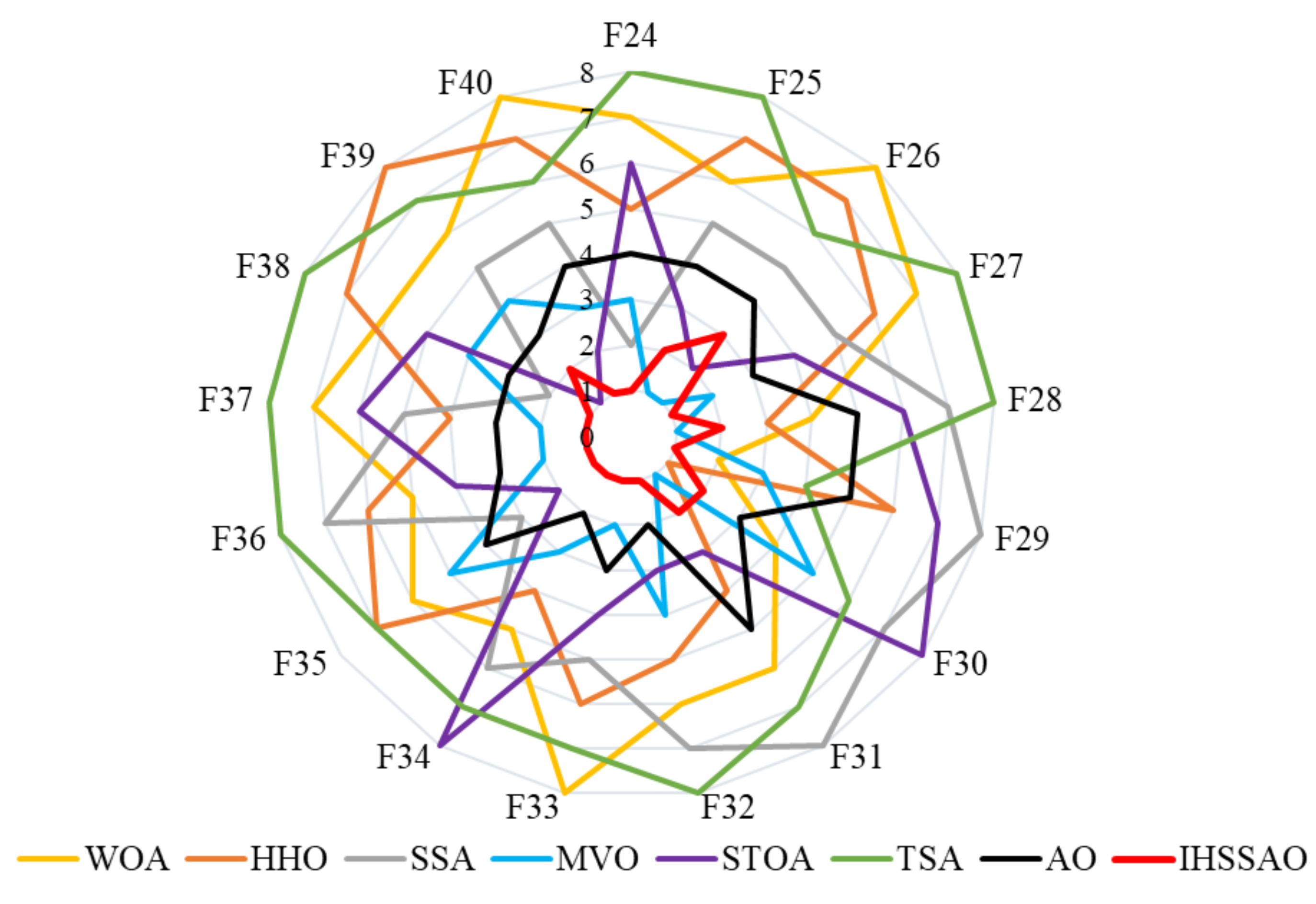
4.2. Experiment II: IEEE CEC2017 Test Functions

In the previous section, the performance of the proposed IHSSAO algorithm in handling simple problems was adequately verified by conducting the standard benchmark function. To further demonstrate the performance of the proposed algorithm in dealing with complex problems, in this section we have chosen the 17 IEEE CECE 2017 test functions, which contain simple multimodal functions, hybrid functions, and composite functions, as listed in

Table 8. Descriptions of 17 selected IEEE CEC2017 test functions.

Function	Name	Dim	Range	Fmin
Simple multimodal functions
F24	Shifted and Rotated Rosenbrock’s Function	10	[−100, 100]	400
F25	Shifted and Rotated Rastrigin’s Function	10	[−100, 100]	500
F26	Shifted and Rotated Expanded Scaffer’s F6 Function	10	[−100, 100]	600
F27	Shifted and Rotated Non-Continuous Rastrigin’s Function	10	[−100, 100]	800
Hybrid functions
F28	Hybrid Function 1 (N = 3)	10	[−100, 100]	1100
F29	Hybrid Function 3 (N = 3)	10	[−100, 100]	1300
F30	Hybrid Function 4 (N = 4)	10	[−100, 100]	1400
F31	Hybrid Function 5 (N = 4)	10	[−100, 100]	1500
F32	Hybrid Function 6 (N = 5)	10	[−100, 100]	1700
F33	Hybrid Function 6 (N = 6)	10	[−100, 100]	2000
Composite Functions
F34	Composition Function 2 (N = 3)	10	[−100, 100]	2200
F35	Composition Function 3 (N = 4)	10	[−100, 100]	2300
F36	Composition Function 4 (N = 4)	10	[−100, 100]	2400
F37	Composition Function 5 (N = 5)	10	[−100, 100]	2500
F38	Composition Function 6 (N = 5)	10	[−100, 100]	2600
F39	Composition Function 7 (N = 6)	10	[−100, 100]	2700
F40	Composition Function 9 (N = 3)	10	[−100, 100]	2900

. To demonstrate the superiority of the IHSSAO, the experimental results of the proposed IHSSAO are evaluated in comparison with the basic SSA, AO, and the five famous algorithms used in the previous section, namely WOA, HHO, MVO, STOA, and TSA. Using the same methodology as the experiments in the previous section, each algorithm is run 30 times with 500 iterations each. The eventual results of the average and standard deviation are listed in

Table 9. Comparative results of HSSAO and other algorithms on 17 CEC2017 functions.

Fn	Metric	WOA	HHO	SSA	MVO	STOA	TSA	AO	IHSSAO
F24	Mean	4.50 × 102	4.37 × 102	4.19 × 102	4.22 × 102	4.44 × 102	5.37 × 102	4.29 × 102	4.18 × 102
	Std	5.10 × 101	3.92 × 101	2.55 × 101	1.73 × 101	2.86 × 101	1.49 × 102	3.49 × 101	2.44 × 101
F25	Mean	5.54 × 102	5.60 × 102	5.37 × 102	5.22 × 102	5.31 × 102	5.60 × 102	5.35 × 102	5.29 × 102
	Std	2.04 × 101	1.52 × 101	1.42 × 101	1.41 × 101	1.08 × 101	2.15 × 101	1.34 × 101	1.12 × 101
F26	Mean	6.43 × 102	6.42 × 102	6.21 × 102	6.12 × 102	6.15 × 102	6.37 × 102	6.20 × 102	6.19 × 102
	Std	1.16 × 101	8.50 × 100	1.42 × 101	4.67 × 100	6.75 × 100	1.51 × 101	7.58 × 100	6.38 × 100
F27	Mean	8.40 × 102	8.33 × 102	8.32 × 102	8.26 × 102	8.31 × 102	8.53 × 102	8.30 × 102	8.25 × 102
	Std	1.34 × 101	1.14 × 101	1.46 × 101	9.95 × 100	9.50 × 100	1.97 × 101	9.01 × 100	6.95 × 100
F28	Mean	1.24 × 103	1.21 × 103	1.29 × 103	1.16 × 103	1.27 × 103	3.95 × 103	1.25 × 103	1.19 × 103
	Std	9.53 × 101	6.19 × 101	1.66 × 102	3.52 × 101	9.64 × 101	2.75 × 103	1.91 × 102	8.29 × 101
F29	Mean	1.62 × 104	2.08 × 104	3.63 × 104	1.67 × 104	2.37 × 104	1.71 × 106	2.00 × 104	1.49 × 104
	Std	1.24 × 104	1.50 × 104	4.62 × 104	1.48 × 104	1.56 × 104	5.19 × 106	1.43 × 104	1.07 × 104
F30	Mean	2.89 × 103	1.84 × 103	5.10 × 103	3.41 × 103	5.19 × 103	4.23 × 103	2.81 × 103	2.30 × 103
	Std	1.51 × 103	5.71 × 102	8.37 × 103	2.90 × 103	4.29 × 103	1.99 × 103	2.18 × 103	1.18 × 103
F31	Mean	1.03 × 104	7.22 × 103	1.32 × 104	2.52 × 103	6.17 × 103	1.14 × 104	7.66 × 103	5.87 × 103
	Std	8.92 × 103	3.30 × 103	1.57 × 104	1.89 × 103	4.23 × 103	9.14 × 103	4.54 × 103	2.68 × 103
F32	Mean	1.81 × 103	1.80 × 103	1.82 × 103	1.79 × 103	1.78 × 103	1.85 × 103	1.78 × 103	1.75 × 103
	Std	6.61 × 101	9.01 × 101	7.58 × 101	5.61 × 101	3.93 × 101	1.01 × 102	3.05 × 101	2.47 × 101
F33	Mean	2.22 × 103	2.17 × 103	2.15 × 103	2.13 × 103	2.15 × 103	2.20 × 103	2.14 × 103	2.12 × 103
	Std	7.67 × 101	6.23 × 101	7.84 × 101	6.98 × 101	7.15 × 101	6.13 × 101	5.96 × 101	4.28 × 101
F34	Mean	2.40 × 103	2.39 × 103	2.44 × 103	2.35 × 103	2.90 × 103	2.64 × 103	2.31 × 103	2.28 × 103
	Std	2.91 × 102	3.26 × 102	3.61 × 102	1.96 × 102	6.75 × 102	3.79 × 102	1.46 × 101	1.03 × 101
F35	Mean	2.67 × 103	2.68 × 103	2.65 × 103	2.66 × 103	2.64 × 103	2.71 × 103	2.65 × 103	2.63 × 103
	Std	3.08 × 101	2.49 × 101	1.36 × 101	3.40 × 101	1.55 × 101	4.05 × 101	2.17 × 101	1.10 × 101
F36	Mean	2.77 × 103	2.78 × 103	2.79 × 103	2.75 × 103	2.76 × 103	2.82 × 103	2.75 × 103	2.74 × 103
	Std	5.46 × 101	1.37 × 102	6.99 × 101	6.44 × 101	1.03 × 101	4.71 × 101	7.79 × 101	9.31 × 101
F37	Mean	2.96 × 103	2.94 × 103	2.94 × 103	2.93 × 103	2.95 × 103	3.08 × 103	2.93 × 103	2.93 × 103
	Std	2.26 × 101	1.97 × 101	3.33 × 101	3.39 × 101	1.78 × 101	1.46 × 102	2.37 × 101	2.85 × 101
F38	Mean	3.59 × 103	3.70 × 103	3.06 × 103	3.17 × 103	3.40 × 103	3.81 × 103	3.07 × 103	3.02 × 103
	Std	5.53 × 102	6.43 × 102	3.87 × 102	4.41 × 102	4.74 × 102	5.67 × 102	2.31 × 102	2.24 × 102
F39	Mean	3.15 × 103	3.20 × 103	3.14 × 103	3.12 × 103	3.10 × 103	3.19 × 103	3.11 × 103	3.10 × 103
	Std	4.24 × 101	5.91 × 101	6.34 × 101	3.09 × 101	2.59 × 100	4.75 × 101	5.94 × 100	1.26 × 101
F40	Mean	3.42 × 103	3.38 × 103	3.29 × 103	3.26 × 103	3.25 × 103	3.34 × 103	3.28 × 103	3.24 × 103
	Std	1.23 × 102	9.08 × 101	8.14 × 101	7.89 × 101	8.40 × 101	1.18 × 102	6.74 × 101	4.18 × 101

The best result obtained is highlighted in bold.

.

According to the experimental results in Table 9, we count the average ranking of the eight algorithms as shown in

Table 10. Rankings of IHSSAO and other algorithms on 17 CEC2017 functions.

Fn	WOA	HHO	SSA	MVO	STOA	TSA	AO	IHSSAO
F24	7	5	2	3	6	8	4	1
F25	6	7	5	1	3	8	4	2
F26	8	7	5	1	2	6	4	3
F27	7	6	5	2	4	8	3	1
F28	4	3	7	1	6	8	5	2
F29	2	6	8	3	7	4	5	1
F30	4	1	7	5	8	6	3	2
F31	6	4	8	1	3	7	5	2
F32	6	5	7	4	3	8	2	1
F33	8	6	5	2	4	7	3	1
F34	5	4	6	3	8	7	2	1
F35	6	7	3	5	2	7	4	1
F36	5	6	7	2	4	8	3	1
F37	7	4	5	2	6	8	3	1
F38	6	7	2	4	5	8	3	1
F39	6	8	5	4	1	7	3	2
F40	8	7	5	3	2	6	4	1

. Moreover, Figure 8 presents the ranking radar diagram of the eight algorithms. Combining Table 9 and Table 10 and Figure 8, we can observe that the IHSSAO can be ranked first on the average in most cases. For the functions $F_{25}$, $F_{28}$, $F_{30}–F_{31}$, and $F_{39}$, the proposed algorithms rank second. Furthermore, for function $F_{26}$, IHSSAO ranks third after MVO and STOA, but there is no significant difference between the first two algorithms.

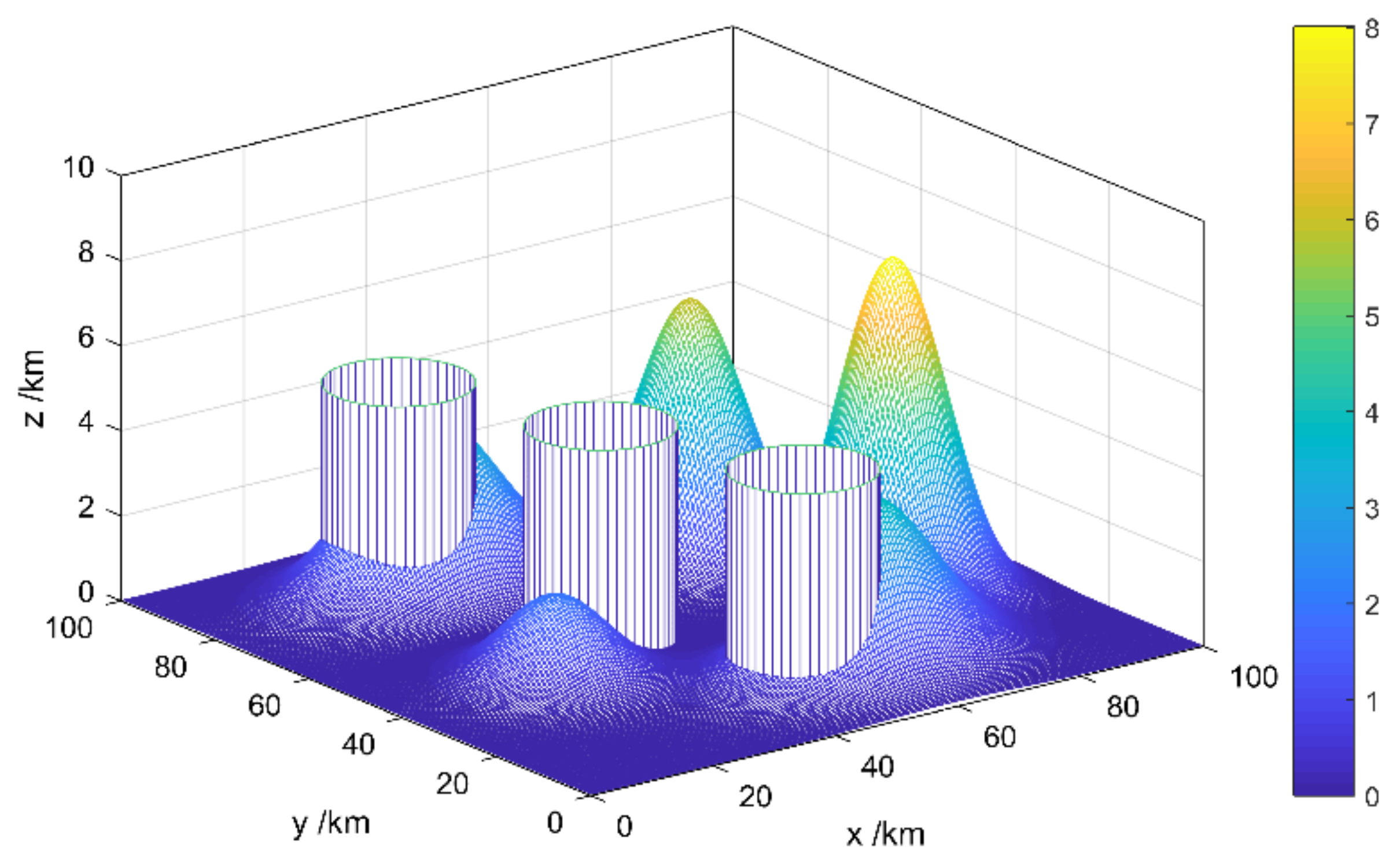
5. IHSSAO for Solving UAV Path Planning in Complex Terrain

5.1. UAV Mission Environment Modeling

When modeling the mission environment for the UAV, we should take essential factors such as the terrain situation and threat situation of the mission into consideration. In this paper, the basic terrain constraints and threat constraints (radar threat, artillery threat, etc.) are mathematically modeled. The specific mission environment modeling approach is as follows.

5.1.1. Terrain Constraints

In various missions, the workspace for UAVs is different. According to the altitude, the terrain is divided into three types of terrain: plain areas, mountainous areas, and hilly areas. One of the most influential factors is the mountain peaks, and the influence of altitude change needs to be considered. Therefore, the model established in this paper is for UAV path planning in complex terrain including mountain peaks. The mathematical expression of the mountain peak model is:

$$Z\left(x,y\right)=h\cdot e^{\left[-\frac{{\left(x-x_0\right)}^2}{m_1}-\frac{{\left(x-y_0\right)}^2}{m_1}\right]}$$

(28)

where $\left(x,y\right)$ is the coordinate of the peak terrain in the horizontal plane; $\left(x_0,y_0\right)$ is the center point coordinate of the peak terrain in the horizontal plane; $h$ represents the height parameter; and $m_1$ and $m_2$ reflect the steepness of the peak.

5.1.2. Threat Constraints

The main threats faced by UAVs in their missions include radar threats, electromagnetic threats, and missile threats. In order to simplify the UAV mission environment model, the cylindrical area with radius $R_i$ is used to represent the threat area, whose radius size determines the coverage of the threat area.

Based on the above conditions, we model the simulation scene of the UAV path planning workspace as depicted in Figure 9.

5.2. UAV Path Planning Modeling

In order to plan a high-quality flight trajectory that satisfies the constraints, it is necessary to establish a suitable fitness function and consider various constraints. The major indicators that affect the performance of UAVs include trajectory length, flight altitude, minimum step length, turning angle cost, maximum climb angle, etc. According to the above UAV flight trajectory constraint, the expression of the cost function is as follows [2]:

$$J_{cost}={\omega }_1{J}_{path}+{\omega }_2{J}_{height}+{\omega }_3{J}_{turn},\left({\omega }_1+{\omega }_2+{\omega }_3=1; {\omega }_i\ge 0\right)$$

(29)

where $J_{cost}$ is the total cost function and the parameters ${\omega }_i, i=1,2,3$ represent the weights of each cost function and satisfy ${\omega }_1+{\omega }_2+{\omega }_3=1$ and ${\omega }_i\ge 0$. $J_{path}$, $J_{height}$, and $J_{turn}$ represent the path length cost, flight altitude cost, and corner cost of UAV, respectively.

The length of the trajectory is also very significant for most flight missions in the UAV path planning process. As we all know, shorter paths save more fuel and more time, and have a lower chance of finding unknown threats. Assuming that there are $n$ waypoints in a complete path, the path cost expression is as follows:

$$\begin{array}{l}{J}_{path}=\left\{\begin{array}{l}\infty , pass the obstacles\\ {\displaystyle \sum _{i=1}^{n-1}{l}_i}, otherwise\end{array}\right.\\ l_i={‖\left(x_{i+1},y_{i+1},z_{i+1}\right)-\left(x_i,y_i,z_i\right)‖}_2\end{array}$$

(30)

where $l_i$ denotes the distance between the $i\mathrm{th}$ waypoint and the $i+1\mathrm{th}$ waypoint. Furthermore, $\left(x_i, y_i, z_i\right)$ and $\left(x_{i+1}, y_{i+1}, z_{i+1}\right)$ are the coordinates of the $i\mathrm{th}$ waypoint and $i+1\mathrm{th}$ waypoint, respectively.

In general, if the UAV is flying at a low altitude in complex mountain terrain, it will easily collide with the grounds and mountains. However, if the UAV flight height is too high, it will also increase fuel costs and the risk of being detected by radar. Therefore, it is very essential for the UAV to keep a stable flight altitude. In order to have a safe UAV flight, we give the following flight height cost $J_{height}$ model.

$$\begin{array}{l}{J}_{height}=\sqrt{\frac{1}{n}{\displaystyle \sum _{i=0}^{n-1}{\left(z{\left(i\right)}^2-\overline{z}\right)}^2}}\\ \overline{z}=\frac{1}{n}{\displaystyle \sum _{i=0}^{n-1}z\left(i\right)}\end{array}$$

(31)

Furthermore, the maneuverability of UAVs is also limited by their turning angle cost function. During the UAV’s mission, its turning angle should be less than or equal to the pre-set maximum turning angle $\varphi$, because the size of the turning angle affects the stability of its flight. The cost function model of turning angle is described as follows.

$$\begin{array}{l}{J}_{turn}=\left\{\begin{array}{l}\infty , if \varphi <{\theta }_i\\ {\displaystyle \sum _{i=1}^n\left(\cos \varphi -\cos {\theta }_i\right), otherwise}\end{array}\right.\\ \cos \theta =\frac{a_i^T{a}_{i+1}}{\left|a_i\right|\left|a_{i+1}\right|}\end{array}$$

(32)

where ${\theta }_i$ represents the $i\mathrm{th}$ turning angle and $a_i$ denotes a vector of the $i\mathrm{th}$ part of the whole path.

By efficiently processing the total cost function, we can obtain the trajectory consisting of line segments. It is undeniable that the obtained paths are often only theoretically feasible, but for practical flyability, it is necessary to smooth the paths Smoothing. In this paper, we apply cubic spline interpolation to smooth the flight trajectory of UAVs.

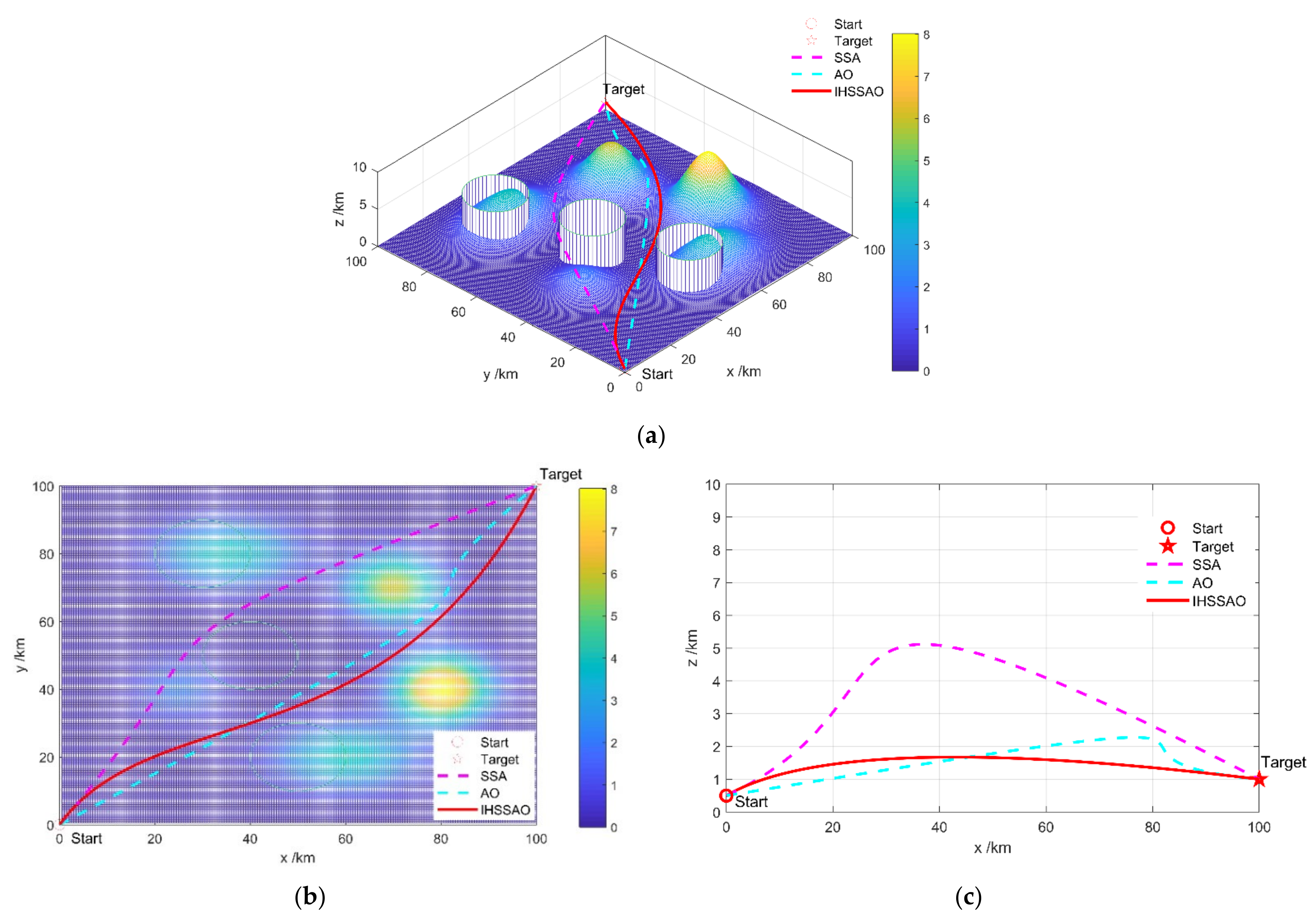
5.3. Simulation Results and Analysis of UAV Path Planning in Complex Terrain

5.3.1. Parameter Settings

The simulation is conducted in MATLAB R2022a in Microsoft Windows 10 with a computer hardware platform configuration of Intel^® Core^TM i7-9750H @ 2.60 GH and RAM 16 G. The workspace of UAV is $\left[0,100\right]$ km long, $\left[0,100\right]$ km wide, and $\left[0,10\right]$ km high. The UAV starting point coordinate is (0, 0, 0.5), and the target point coordinate is (200, 200, 1). The simulation scene of the UAV path planning workspace is depicted in Figure 9. The plane coordinates and radius of the three threat area centers are shown in

Table 11. Parameter settings of the threat area.

Threat Sequence	Center Coordinates (km)	Radius (km)
1	(60, 160)	20
2	(80, 100)	20
3	(100, 40)	20

. Moreover, the maximum turning angles $\varphi ={60}^{°}$, ${\omega }_1$, ${\omega }_2$, and ${\omega }_3$ are 0.4, 0.4, and 0.2, respectively.

In this experiment, we use the basic SSA and AO to compare with the proposed IHSSAO. For all these algorithms, the population number and the maximum number of iterations are set to 30 and 50, respectively.

5.3.2. Simulation Results and Analysis

Figure 10 demonstrates the trajectory of the UAV in complex terrain. The comparison of the basic SSA, AO, and the proposed IHSSAO in the UAV planning path map shows that although the basic SSA can avoid the threat area as well as the AO and IHSSAO algorithms, its planned path is not only too high in the flight altitude, but also too long in the flight path, and consumes more energy. On the other hand, although the UAV path planned by the AO met all aspects of the UAV constraints in the early stage, the flight altitude variation was large and the pitch angle was too large at the location near the back row of peaks. Compared with the basic SSA and AO, the IHSSAO proposed in this paper can plan an optimal trajectory that avoids mountainous terrain and threat areas, and can fly as close to the ground as possible while satisfying the physical constraints of the UAV.

Furthermore, Figure 11 shows the convergence cures of the SSA, AO, and IHSSAO. According to the simulation results, we can observe that IHSSAO not only has a rapid convergence rate but also has the best convergence effect. Although it falls into a local optimum in the early stage, the proposed algorithm can escape from the local optimum due to the fact that we introduced the pinhole imaging opposition-based learning strategy into it. In conclusion, the proposed IHSSAO has superiority over the basic SSA and AO in solving the UAV path planning problem in complex terrain.

6. Conclusions

In this study, we propose a novel improved hybrid Salp Swarm Algorithm and Aquila Optimizer called IHSSAO for UAV path planning in complex terrain. Firstly, the tent chaotic map is introduced into the proposed algorithm with the aim of randomly generating the initial population and increasing the diversity of the initial individuals. Secondly, aiming to enable the search individuals to fully utilize the information of the optimal solution and enhance the global search capability of the proposed algorithm, we integrate the leader mechanism of SSA into the position update formulation of the basic AO. Thirdly, we introduced the pinhole imaging opposition-based learning into the proposed algorithm to increase the diversity of search positions and enhance the ability to get rid of the local optimum. In order to evaluate the performance of the proposed algorithm, IHSSAO is compared with the basic SSA, AO, and five other advanced meta-heuristic algorithms based on 23 classical benchmark functions and 17 IEEE CEC2017 test functions. Experimental results indicate that the proposed IHSSAO algorithm is superior to the basic SSA, AO, and five other advanced meta-heuristic algorithms in the global optimization. Eventually, we apply the proposed IHSSAO to solve the UAV path planning problem in complex terrain. The experimental result demonstrates that the path planned by the proposed IHSSAO is more consistent with the mission requirements and various constraints than the basic SSA and AO in the same environment.

In the future, to validate the performance of IHSSAO, we will introduce more constraints, such as flight speed constraints and dynamic obstacles. In addition, we can attempt to further enhance the proposed algorithm and apply it to fault diagnosis for aero engines and formation control of multi-UAVs.

References

1. Pan, J.-S.; Lv, J.-X.; Yan, L.-J.; Weng, S.-W.; Chu, S.-C.; Xue, J.-K. Golden eagle optimizer with double learning strategies for 3D path planning of UAV in power inspection. Math. Comput. Simul. 2022, 193, 509–532. [Google Scholar] [CrossRef]
2. Liu, G.Y.; Shu, C.; Liang, Z.W.; Peng, B.H.; Cheng, L.F. A Modified Sparrow Search Algorithm with Application in 3d Route Planning for UAV. Sensors 2021, 21, 1224. [Google Scholar] [CrossRef] [PubMed]
3. Song, Q.S.; Li, S.B.; Yang, J.; Bai, Q.; Hu, J.J.; Zhang, X.X.; Zhang, A.S. Intelligent Optimization Algorithm-Based Path Planning for a Mobile Robot. Comput. Intell. Neurosci. 2021, 2021, 8025730. [Google Scholar] [CrossRef]
4. Huang, C.; Fei, J.Y. UAV Path Planning Based on Particle Swarm Optimization with Global Best Path Competition. Int. J. Pattern Recognit. Artif. Intell. 2018, 32, 1859008. [Google Scholar] [CrossRef]
5. Kobayashi, M.; Motoi, N. Local Path Planning: Dynamic Window Approach with Virtual Manipulators Considering Dynamic Obstacles. IEEE Access 2022, 10, 17018–17029. [Google Scholar] [CrossRef]
6. Tang, Y.; Miao, Y.M.; Barnawi, A.; Alzahrani, B.; Alotaibi, R.; Hwang, K. A joint global and local path planning optimization for UAV task scheduling towards crowd air monitoring. Comput. Netw. 2021, 193, 107913. [Google Scholar] [CrossRef]
7. Salama, O.A.A.; Eltaib, M.E.H.; Mohamed, H.A.; Salah, O. RCD: Radial Cell Decomposition Algorithm for Mobile Robot Path Planning. IEEE Access 2021, 9, 149982–149992. [Google Scholar] [CrossRef]
8. Yuan, X.; Yuan, X.W.; Wang, X.H. Path Planning for Mobile Robot Based on Improved Bat Algorithm. Sensors 2021, 21, 4389. [Google Scholar] [CrossRef]
9. Zhou, C.M.; Huang, B.D.; Franti, P. A review of motion planning algorithms for intelligent robots. J. Intell. Manuf. 2022, 33, 387–424. [Google Scholar] [CrossRef]
10. Yang, S.X.; Meng, M. An efficient neural network approach to dynamic robot motion planning. Neural Netw. 2000, 13, 143–148. [Google Scholar] [CrossRef]
11. Smart, W.D.; Kaelbling, L.P. Effective reinforcement learning for mobile robots. In Proceedings of the 2002 IEEE International Conference on Robotics and Automation, Washington, DC, USA, 11–15 May 2002; pp. 3404–3410. [Google Scholar]
12. Mirjalili, S. The Ant Lion Optimizer. Adv. Eng. Softw. 2015, 83, 80–98. [Google Scholar] [CrossRef]
13. Mirjalili, S.; Lewis, A. The Whale Optimization Algorithm. Adv. Eng. Softw. 2016, 95, 51–67. [Google Scholar] [CrossRef]
14. Heidari, A.A.; Mirjalili, S.; Faris, H.; Aljarah, I.; Mafarja, M.; Chen, H.L. Harris hawks optimization: Algorithm and applications. Future Gener. Comput. Syst.-Int. J. Esci. 2019, 97, 849–872. [Google Scholar] [CrossRef]
15. Mirjalili, S.; Mirjalili, S.M.; Lewis, A. Grey Wolf Optimizer. Adv. Eng. Softw. 2014, 69, 46–61. [Google Scholar] [CrossRef] [Green Version]
16. Mirjalili, S.; Gandomi, A.H.; Mirjalili, S.Z.; Saremi, S.; Faris, H.; Mirjalili, S.M. Salp Swarm Algorithm: A bio-inspired optimizer for engineering design problems. Adv. Eng. Softw. 2017, 114, 163–191. [Google Scholar] [CrossRef]
17. Qu, C.Z.; Gai, W.D.; Zhong, M.Y.; Zhang, J. A novel reinforcement learning based grey wolf optimizer algorithm for unmanned aerial vehicles (UAVs) path planning. Appl. Soft Comput. 2020, 89, 106099. [Google Scholar] [CrossRef]
18. Lv, J.X.; Yan, L.J.; Chu, S.C.; Cai, Z.M.; Pan, J.S.; He, X.K.; Xue, J.K. A new hybrid algorithm based on golden eagle optimizer and grey wolf optimizer for 3D path planning of multiple UAVs in power inspection. Neural Comput. Appl. 2022. [Google Scholar] [CrossRef]
19. Xiao, Y.; Sun, X.; Guo, Y.; Cui, H.; Wang, Y.; Li, J.; Li, S. An enhanced honey badger algorithm based on Lévy flight and refraction opposition-based learning for engineering design problems. J. Intell. Fuzzy Syst. 2022, 1–24. [Google Scholar] [CrossRef]
20. Xiao, Y.; Sun, X.; Guo, Y.; Li, S.; Zhang, Y.; Wang, Y. An improved gorilla troops optimizer based on lens opposition-based learning and adaptive β-Hill climbing for global optimization. CMES-Comp. Model. Eng. Sci. 2022, 131, 815–850. [Google Scholar] [CrossRef]
21. Huo, L.S.; Zhu, J.H.; Li, Z.M.; Ma, M.H. A Hybrid Differential Symbiotic Organisms Search Algorithm for UAV Path Planning. Sensors 2021, 21, 3037. [Google Scholar] [CrossRef]
22. Ji, Y.S.; Zhao, X.C.; Hao, J.L. A Novel UAV Path Planning Algorithm Based on Double-Dynamic Biogeography-Based Learning Particle Swarm Optimization. Mob. Inf. Syst. 2022, 2022, 8519708. [Google Scholar] [CrossRef]
23. Abualigah, L.; Yousri, D.; Abd Elaziz, M.; Ewees, A.A.; Al-qaness, M.A.A.; Gandomi, A.H. Aquila Optimizer: A novel meta-heuristic optimization algorithm. Comput. Ind. Eng. 2021, 157, 107250. [Google Scholar] [CrossRef]
24. AlRassas, A.M.; Al-qaness, M.A.A.; Ewees, A.A.; Ren, S.R.; Abd Elaziz, M.; Damasevicius, R.; Krilavicius, T. Optimized ANFIS Model Using Aquila Optimizer for Oil Production Forecasting. Processes 2021, 9, 1194. [Google Scholar] [CrossRef]
25. Ma, L.; Li, J.; Zhao, Y. Population Forecast of China’s Rural Community Based on CFANGBM and Improved Aquila Optimizer Algorithm. Fractal Fract. 2021, 5, 190. [Google Scholar] [CrossRef]
26. Kandan, M.; Krishnamurthy, A.; Selvi, S.A.M.; Sikkandar, M.Y.; Aboamer, M.A.; Tamilvizhi, T. Quasi oppositional Aquila optimizer-based task scheduling approach in an IoT enabled cloud environment. J. Supercomput. 2022, 78, 10176–10190. [Google Scholar] [CrossRef]
27. Fan, Q.; Chen, Z.J.; Zhang, W.; Fang, X.H. ESSAWOA: Enhanced Whale Optimization Algorithm integrated with Salp Swarm Algorithm for global optimization. Eng. Comput. 2022, 38, 797–814. [Google Scholar] [CrossRef]
28. Li, Y.C.; Han, M.X.; Guo, Q.L. Modified Whale Optimization Algorithm Based on Tent Chaotic Mapping and Its Application in Structural Optimization. Ksce J. Civ. Eng. 2020, 24, 3703–3713. [Google Scholar] [CrossRef]
29. Zhang, Z.X.; Yang, R.N.; Li, H.Y.; Fang, Y.H.; Huang, Z.Y.; Zhang, Y. Antlion optimizer algorithm based on chaos search and its application. J. Syst. Eng. Electron. 2019, 30, 352–365. [Google Scholar] [CrossRef]
30. Huang, Y.H.; Zhang, J.; Wei, W.; Qin, T.; Fan, Y.C.; Luo, X.M.; Yang, J. Research on Coverage Optimization in a WSN Based on an Improved COOT Bird Algorithm. Sensors 2022, 22, 3383. [Google Scholar] [CrossRef]
31. Khajehzadeh, M.; Taha, M.R.; Eslami, M. Opposition-based firefly algorithm for earth slope stability evaluation. China Ocean. Eng. 2014, 28, 713–724. [Google Scholar] [CrossRef]
32. Wang, Z.S.; Ding, H.W.; Yang, J.J.; Wang, J.; Li, B.; Yang, Z.J.; Hou, P. Advanced orthogonal opposition-based learning-driven dynamic salp swarm algorithm: Framework and case studies. IET Control. Theory Appl. 2022, 16, 945–971. [Google Scholar] [CrossRef]
33. Zhang, D.M.; Xu, H.; Wang, Y.R.; Song, T.T.; Wang, L.Q. Whale optimization algorithm for embedded Circle mapping and onedimensional oppositional learning based small hole imaging. Kongzhi Yu Juece/Control. Decis. 2021, 36, 1173–1180. [Google Scholar] [CrossRef]
34. Mirjalili, S.; Mirjalili, S.M.; Hatamlou, A. Multi-verse optimizer: A nature-inspired algorithm for global optimization. Neural Comput. Appl. 2015, 27, 495–513. [Google Scholar] [CrossRef]
35. Dhiman, G.; Kaur, A. STOA: A bio-inspired based optimization algorithm for industrial engineering problems. Eng. Appl. Artif. Intell. 2019, 82, 148–174. [Google Scholar] [CrossRef]
36. Kaur, S.; Awasthi, L.K.; Sangal, A.L.; Dhiman, G. Tunicate swarm algorithm: A new bio-inspired based metaheuristic paradigm for global optimization. Eng. Appl. Artif. Intell. 2020, 90, 103541. [Google Scholar] [CrossRef]
Figure 1. Individual salp and swarm of salps.
Applsci 12 05634 g001
Figure 2. Distribution histogram of logistic chaotic map and tent chaotic map. (a) Logistic chaotic map. (b)Tent chaotic map.
Applsci 12 05634 g002
Figure 3. Principle of pinhole imaging opposition-based learning.
Applsci 12 05634 g003
Figure 4. Flow chart of the proposed IHSSAO.
Applsci 12 05634 g004
Figure 5. Three-dimensional view of the search space for 23 benchmark functions. (a) Unimodal benchmark function, benchmark functions. (b) Multimodal benchmark function, benchmark functions. (c) Fix-dimension multimodal benchmark function, benchmark functions.
Applsci 12 05634 g005
Figure 6. Boxplot of IHSSAO and other different algorithms on 23 benchmark functions.
Applsci 12 05634 g006aApplsci 12 05634 g006b
Figure 7. Convergence curve of IHSSAO and other different algorithms on 23 benchmark functions.
Applsci 12 05634 g007aApplsci 12 05634 g007b
Figure 8. Radar ranking diagram of the nine algorithms on 17 CEC2017 functions.
Applsci 12 05634 g008
Figure 9. UAV path planning workspace in complex terrain.
Applsci 12 05634 g009
Figure 10. The best path of SSA, AO, and IHSSAO. (a) Path comparison in three-dimensional space. (b) Path comparison of paths in the X-Y plane. (c) Side view of path comparison in the X-Z plane.
Applsci 12 05634 g010
Figure 11. The convergence cures of the SSA, AO, and IHSSAO.
Applsci 12 05634 g011