Abstract
Tunneling in mixed ground often results in severe torque fluctuations and a low advance rate. Therefore, choosing a reasonable set of parameters for accurate advance rate prediction is paramount to reduce cutter wear and improve tunneling efficiency. However, since the geological parameters in mixed ground conditions are diverse and uncertain, the prediction of the advance rate (AR) of EPB shield tunneling is significantly more difficult than that in homogeneous ground (i.e., full-face hard-rock ground). In addition, the operating parameters of the EPB shield tunneling can be subjective and suboptimal, and each of them has some intricate influence on AR. In this paper, an optimized back-propagation neural network by genetic algorithm (BPNN-GA) was proposed for reasonable operating parameter selection and accurate AR prediction, and four typical machine learning methods were used for comparison. Five processing strategies with different input parameters were also proposed and compared to determine the optimum selection of geological parameters in mixed ground conditions. The proposed models with strategies were adopted in the case study of the Nanjing Metro Line S6 project, and a total of 1188 rings of datasets were used for this study. The results showed that the proposed modified BPNN with the genetic algorithm could be effectively implemented for the AR prediction. It concluded that Strategy B—i.e., using the composite ratio and the geological parameters of each layer as input—was the best strategy in mixed ground conditions for advance rate prediction. Hence, a high correlation between measured and predicted AR was observed in this study with a correlation coefficient (R2) of 0.920.
1. Introduction
Earth pressure balance (EPB) shield tunneling is extensively used in civil construction for its fast and safe characteristics [1,2]. In the construction of subways and some infrastructure tunnels, the advantages of using EPB shield tunneling over traditional construction methods are significant [3]. However, the use of EPB shield tunneling is highly dependent upon the operators. That is, the operators need to adjust the operating parameters of the shield machine constantly to maintain a reasonable advance rate and control the shield attitude, which is neither efficient nor safe. Furthermore, with the increase in engineering projects, we encounter more and more composite strata, and these are easily found in many engineering projects in southern coastal cities of China, such as Guangzhou, Nanjing, Xiamen, etc. Tunneling in complex and mixed ground conditions often results in accidents [4]. Therefore, it is necessary to determine the influencing factors and implement accurate predictions [5]. With the rapid development of computer technology and applications of machine learning [6], the powerful learning capabilities and modeling capabilities of machine learning appeared. Therefore, this paper will aim to establish a high-precision prediction model of advance rate in mixed ground using machine learning method, and propose feasible suggestions for parameter selection in the current research.
In the past, there were many detailed studies conducted on the excavation process and stress state of the tunnel shield machine. In that period, many theoretical and empirical formulas were proposed. The most famous model is the Colorado School of Mines (CSM) model [7]. This model comprehensively considered rock mass parameters such as uniaxial compressive strength and tensile strength, as well as cutter characteristics. In recent years, some models that use more data and more factors have also been proposed. Shi et al. [8] proposed a theoretical model which considered several factors that are responsible for the resistance torque. Kim et al. [9] did a lot of tests, and found a link between thrust and torque. Zhao et al. [10] proposed a model that connected the cutterhead torque with the penetration. It proved that the parameters on the EPB shield tunneling did have some inner relationship. However, too much simplification is used in these models mentioned above, which means that these models need a lot of empirical parameters, and this may make them unable to accurately predict the parameters of the shield machine, cause safety hazards, or require more time.
Numerical simulations based on finite difference and finite element methods, as a popular method in modern times, can effectively simulate the shield tunneling process, and then the force and deformation at different times and states can be obtained. Alsahly et al. [11] proposed a computational framework for the simulation of the advancement and the excavation process of tunnel boring machines (TBM) in mechanized tunneling. Lee et al. [12], using a coupled discrete element method (DEM) and a finite difference method (FDM), simulated EPB shield tunneling and the torque, thrust, chamber pressure, discharge, and settlement data were successfully simulated. However, due to the large amount of calculation in numerical simulation, the calculated results are only applicable to specific strata, and implementing additional models is necessary for different strata to reduce the robustness of the model, which make it unable to be used in mixed ground conditions.
In addition to the two methods above, artificial intelligence methods have also played a vital role in the construction field in recent years. Machine learning (ML) advances the traditional observational method by employing data analysis and pattern recognition techniques, so the nonlinear relationship between shield tunneling parameters can be analyzed, which can make the model show the high levels of accuracy [13]. In the machine learning area, Yagiz et al. [14], Mobarra et al. [15], Salimi [16], and Koopialipoor et al. [17] used artificial neural networks (ANNs) or deep neural networks (DNNs) to predict the penetration rate of the TBMs and could realize a highly accurate estimation. Chen et al. [18] compared the accuracy and computational time of back-propagation neural network (BPNN), radial basis function neural network (RBFNN), and general regression neural network (GRNN), showing the power of neural networks. In order to cover the time series effect of shield tunneling data, Gao et al. [19] and Chen et al. [20] used long-short term memory (LSTM) networks, which can combine the previous learning information with the current input to generate the current output and it can effectively overcome the drawback of gradient explosion or gradient vanish caused by recurrent neural networks (RNNs). Lin et al. [6] presented a hybrid model that used particle swarm optimization (PSO) algorithm to determine the hyperparameters for the LSTM neural network which performed better than the single model of LSTM. Despite all of the aforementioned studies, it is believed that machine learning can achieve good predictions of shield tunneling parameters.
Though great advances have been made in shield tunneling parameters prediction, most of these studies focus on a single formation, which means the geological conditions do not change much or even change with the advancement of shield tunneling. However, the mixed ground, as one of the adverse geological conditions [2], is very common in engineering. Adverse geological conditions can strongly affect TBM advance rate and cutter wear, therefore it is necessary to propose a model that can predict the construction parameters of shield tunneling under the condition of mixed ground in order to better ensure the safety of shield construction. Wang et al. [5] mentioned that their model was based on mixed ground, but the input parameters in the advance rate predictive model include slurry pressure, cutterhead torque, total thrust, rotation speed, pump pressure of thrust cylinders and flow rate in the feed and return line, and those parameters cannot reflect the effects of mixed ground. Fortunately, some scholars have found some relationships between mixed ground and penetration rate through data analysis, and these findings can provide some inspiration. Tóth et al. [21] obtained a model for calculating the penetration rate of a TBM in a mixed ground; however, the model’s accuracy was not high enough and the method used was only mathematical statistics. Zhou et al. [22] assumed that the mixed-face ground included a general soft ground formation and a hard rock formation simultaneously. Based on this assumption, force on the disc cutters and drag bits can both be calculated separately. Consequently, the torque and friction on the entire shield machine cutterhead can be calculated. Through those previous studies, we believe that it is scientific and feasible to realize the prediction of the advance rate of shield tunneling in mixed ground.
In this study, an advance rate prediction model based on genetic algorithm (GA) and back-propagation neural network (BPNN) was developed, and some other machine learning methods were used for comparison and demonstration. All the methods considered the mixed ground situation and could achieve a high-accuracy prediction. The paper is organized as follows: In Section 2, the methodology of the BPNN and GA is introduced, and the mixed ground strategy for the parameter selection is proposed. In Section 3, the proposed model is applied to a tunnel project in Nanjing for demonstration. In Section 4, corresponding evaluation metrics are used to find the most suitable method for forecasting the advance rate of shield tunneling in mixed ground, and the results are presented. In Section 5, some conclusions and drawbacks of this study are summarized.
2. Methodology and Strategy
The following methods that used in this study include: multiple linear regression (MLR), k-nearest neighbor (KNN), support vector regression (SVR), the classification and regression tree (CART), and back-propagation neural network (BPNN). These algorithms, as well as the genetic algorithm as an optimization, will be introduced in order below. In addition, the parameter preprocessing strategy for mixed ground condition will also be introduced in this section.
2.1. Multivariate Linear Regression
Multivariate linear regression (MLR) is one of the simplest and fastest predictive models. It uses the optimal combination of multiple independent variables to predict or estimate the dependent variable, which is more effective and more practical than using only one independent variable to predict or estimate. The equation is presented as Equation (1):
where y is the output, n is the number of features, di and b are the parameters that can be obtained by the least squares method, xi is the input value.
2.2. K-Nearest Neighbor
K-nearest neighbor regression (KNN) adopts the idea of clustering. It can not only deal with classification problems, but also solve regression problems. The algorithm finds the K-nearest neighbors of a sample and assigns the average value of a certain attribute (some) of these neighbors. Given the sample, the value of the attribute corresponding to the sample can be obtained, thereby obtaining the output value Y. This algorithm is simple and easy to use. It determines the relationship between the target point and each point in the training set by calculating the spatial distance of the multi-dimensional vector, making it suitable for nonlinear problems. The algorithm has also been selected as the top 10 algorithms in data mining [23]. The distance calculation formula used in the K-nearest neighbor algorithm is usually Euclidean distance, which can be defined as Equation (2):
where n is the dimension of the input data, and xi and yi represent the value of the target point and the training set point in each dimension respectively.
2.3. Support Vector Regression
Since Corinna Cortes and Vladimir Vapnik proposed the support-vector network and applied it to the handwritten character recognition problem [24], this method had been used in various fields. Originally, support vector machine was only used for classification problems. Later, some scholars extended it to the field of regression and proposed support vector regression [25]. The algorithm treats all data as one class, and searches for a hyperplane in a high-dimensional space so that the total deviation of the distance from all sample points to the hyperplane is minimized to achieve regression. SVR is quite effective to solve the regression problems of high-dimensional features, and it can still maintain good results when the feature dimension is greater than the number of samples. Additionally, it is not easily affected by noisy data, and overfitting is not prone to occur. The biggest feature of the SVR is that it uses a soft boundary. If the sample point is close enough to the regression model—that is, it falls within the interval boundary of the regression model—the loss is not calculated for the sample, and the corresponding loss function is called ε-insensitive loss function. It can be defined as Equation (3):
where f(x) is the regression function, and ε is a hyperparameter that determines the width of the interval boundary which should be defined by the user.
According to Equation (3), only when the outlier is more than a distance from our regression function will it be included in our function loss; otherwise, it has no effect on the regression equation. As for the regression function, it can be written as
where ωi is the adjustable weight vector and b is the bias, and φi(x) is the kernel which can map the input space into a high-dimensional feature space. The kernel used in this paper is the radial basis function (RBF).
2.4. Classification and Regression Tree
Classification and regression tree (CART) is a regression method for nonparametric classes. It can be used to solve both classification problems and regression problems. CART mainly consists of the following two parts: first, a decision tree is generated based on the training dataset; second, the generated tree is pruned and the optimal subtree is selected. At this time, the minimum loss function is used as the criterion for pruning. CART automatically selects features, allows it to be used with a large number of features, fits certain types of data potentially much better than linear regression, and does not require specialized statistical knowledge for interpretation, so it can be highly effective.
2.5. Back-Propagation Neural Network
Back-propagation neural network (BPNN) is one of the most popular neural networks which was proposed by Rumelhart et al. [26]. Like a neural network, it also consists of an input layer, one or multiple hidden layers, and an output layer, each of which has one or more neurons. The neurons in different layers are connected to each other. After we feed the data into the model, the result of the hidden layer can be calculated by Equation (5):
where xi is the input value, Hj is the result of the hidden neuron j, n is the number of the hidden neuron, ωij is the weight on the connection between the input and the hidden neuron j, aj is the bias from the input layer to the hidden layer, and f is the activation function.
From the hidden layer to the output layer, for the regression model, in most cases, a linear model is used, which can be expressed as Equation (6):
where Hj is the value of the hidden neuron j, yk is the output value of the output neuron k, m is the number of the hidden neuron, ωjk is the weight on the connection between the hidden neuron j and the output neuron k, and bk is the bias from the hidden layer to the output layer.
To account for the nonlinearity, the activation is used in most cases, and in this paper, some famous activation functions such as ‘relu’, ‘tanh’, and ‘sigmoid’ will be used. Those activation functions can be expressed as
where the Input is similar to the process in hidden layer, and e is the natural constant, approximately equal to 2.71828.
When the signal finally reaches the output layer, the model will compare the output result with the real value, and calculate the error between them, and then backpropagate the error to adjust the weights and biases in each layer of neurons until the error of the model is within the acceptable range. This is the core function of BPNN, and over a number of learning cycles (epochs), it can achieve a high-precision prediction [27]. The entire structure of the model is shown in Figure 1.
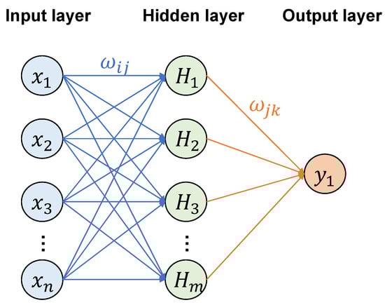
Figure 1.
Neural network structure.
2.6. Genetic Algorithm
Genetic algorithm (GA) was proposed by Holland [28]. It mainly simulates Darwin’s evolution theory of survival of the fittest [29]. GA is usually regarded as an optimization algorithm, where its powerful function enables it to find the optimal solution of a problem in the shortest time [30]. Each solution corresponds to a chromosome, and each parameter on each solution is the gene on the chromosome. In order to select the best solution (chromosome) from many genetic compositions, the GA mainly includes the following six steps.
- Initialization: During the initialization process, the model will randomly select genes from the gene pool to form the chromosome. The random selection will increase the diversity of the population.
- Evaluation: The fitness (cost) function is then used to evaluate each chromosome to determine the fitness value.
- Selection: In this process, the model will select the superior individuals from the group and eliminate the inferior individuals. The purpose is to directly inherit the optimized individuals to the next generation or generate new individuals through pairing and crossover and then inherit them to the next generation, so as to continuously find the optimal one.
- Crossover: Just like genetic recombination in nature, it replaces and recombines part of the genes of two parent individuals to generate a new individual. Through crossover, the search ability of genetic algorithm can be improved by leaps and bounds;
- Mutation: This step will make changes in gene values at certain loci of individual strings of the population, by introducing another level of randomness. This will effectively avoid the model falling into the dilemma of local optimum.
- End: When the fitness of the optimal individual reaches a given threshold, or the fitness of the optimal individual and the fitness of the group no longer rise, or the number of iterations reaches a preset number of generations, the algorithm terminates.
In order to visualize the algorithm, Figure 2 shows the process of using the genetic algorithm to optimize the neural network in this paper. The gene database can be changed so this method can also be used in other fields.
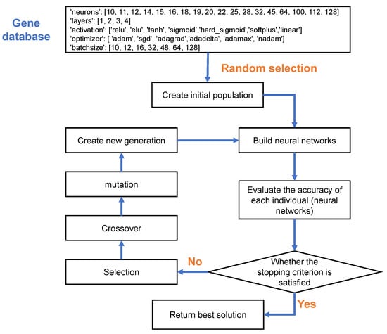
Figure 2.
Flow chart of genetic algorithm.
2.7. Strategies for Mixed Ground
Given that the research on the operating parameters of EPB shield tunneling is mainly concentrated in uniform stratum conditions nowadays, the research on the operating parameters of EPB shield tunneling under the mixed ground condition is relatively backward. However, since mixed ground conditions are a kind of common special geological condition in shield tunnel construction and they appear in a large number of sections in this research—which means there could be more than one geological parameter at the same position during the excavation process—it is necessary to make a reasonable selection of operating parameters of EPB shield tunneling in the mixed ground condition. In the previous literature, Wang et al. [5] mainly analyzed the advance rate data in the mixed ground and compared it with other data in single geological conditions. Lin et al. [6] proposed a network prediction method using PSO combined with LSTM, and applied it to construction projects involving mixed ground geology. For mixed ground, they tended to use the thickness of each layer as a comprehensive method of weighting, but the final effect of this model was not particularly ideal. Therefore, there are prominent problems in this research of how to select more suitable parameters to predict the advance rate of the mixed ground, or how to deal with the geological parameters of the mixed ground to make them become more suitable input parameters for model prediction.
In order to guarantee the accuracy of the prediction model in a single stratum as well as make the prediction model adapt to the situation of mixed ground, the following countermeasures are proposed in this paper, and they are carried out in field verification in Section 4. Most of the tunnel faces during tunneling are composed of two kinds of strata, but a small part is composed of three or more kinds of strata. In order to simplify the calculation and optimize the parameters, this paper will select two dominant strata as upper layer and lower layer data respectively.
Strategy A: Divide each type of geological parameters into two columns. One column represents the rock (soil) geological parameters of the upper part of the mixed ground, and the other represents the lower part geological parameters. Figure 3 shows the parameters of each part. The whole circle represents the face of the shield excavated by the shield tunneling, and the object on the left represents the side view of the cutter head. Su and Sd represent the area of upper strata and lower strata in excavation face separately.
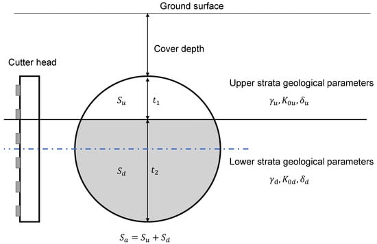
Figure 3.
Diagram of mixed ground. (γ, K0, and δ are the geological parameters that will be introduced later. The dotted line represents the central axis of the shield tunneling).
Strategy B: On the basis of Strategy A, the composite ratio parameter p is added to represent the area proportion of the upper soil layer in the whole tunnel face. It can be expressed in Equation (10):
where Su represents the area of upper strata in excavation face, Sa represents total area of excavation face.
Strategy C: A comprehensive geological index is proposed to represent an overall excavation difficulty of the excavation face. The comprehensive geological index is defined as Equation (11):
where ωi represents comprehensive geological indicators, θi1 is the geological parameters of the upper strata, and θi2 is the geological parameters of the lower strata, θi ∈ {γ, K0, δ}.
Strategy D: Calculate the comprehensive geological index with the thickness of the formation as the weight, which is also a comprehensive geological index that was proposed by Lin et al. [6], as defined by Equation (12):
where t1 represents the thickness of the upper layer, and t2 represents the thickness of the lower layer.
Strategy E: Take the parameters of the two strata on the face that are more likely to hinder the advance rate as the input. As we know, greater uniaxial compressive strength will bring greater obstacles to shield advance. Therefore, in this scheme, the larger geological parameters of the upper and lower layers are used as the input:
Table 1 shows the input and output parameters of the model corresponding to the five strategies. The difference between them is mainly in the selection of geological parameters. In general, the number of input parameters of Strategy A and Strategy B are 12 and 13 respectively. There are nine input parameters for Strategy C, D, and E. The parameter input of each strategy is vividly exhibited in Figure 4.

Table 1.
Input and output parameters of each strategy.
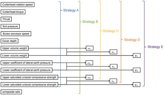
Figure 4.
Input parameters of each strategy.
3. Case Study
3.1. Project Description
In this study, the tunnel construction project between Qilin Town Station and Dongjiao Town Station of Nanjing Rail Transit S6 Line in Nanjing, China was investigated. The underground section of the tunnel is 1342 m long, the maximum buried depth is about 19.97 m. The cover depth of tunnel varies from 10 to 28 m; The shallowest buried depth is located at the long deep highway near the open excavation section, which is only about 2.5 m.
During the excavation process, the EPB shield tunneling will encounter very complex and variable strata. The geological conditions of the longitudinal section of the tunnel can be divided into the following three categories according to the rock strength: ① Full-section soft rock/soil (accounting for 47%), ② full-section hard rock formations (29%), and ③ upper-soft lower-hard composite formations (24%). The ever-changing geological conditions will have a great impact on EPB shield tunneling, leading to great difficulties in the prediction of EPB shield tunneling parameters. Therefore, a high-precision shield tunneling parameter prediction model is urgently needed. The geological profile of the longitudinal section of the tunnel is shown in Figure 5, which clearly shows the various strata that will be encountered during the excavation process. The upper part is mostly clay, silty clay, residual soil, etc. While the lower part is mostly granite or ash with different degrees of weathering. Meanwhile, due to the special geological conditions in Nanjing, there are still individual karst caves in this area. In order to ensure the safety of shield construction, those karst caves were fulfilled with water glass grouting before. The physical and mechanical parameters of each soil layer are presented in Table 2, these parameters play a key role in the operating parameters of the shield tunneling. The geological profile of the shield tunnel approach is shown in Figure 6, and various geological conditions that will be encountered during the excavation process are clearly exhibited.
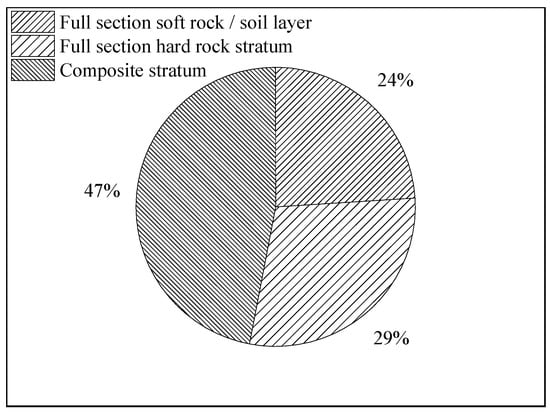
Figure 5.
Proportion of various strata along the longitudinal direction of the tunnel.
Table 2.
Physicomechanical properties of encountered ground types.
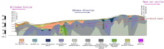
Figure 6.
Geological profile of the tunnel between Qilin Town Station and Dongjiao Town Station.
Facing complex and variable terrain, the DZ423 earth pressure balance shield machine was selected for this construction. The opening rate of the cutter head is about 41%, and the diameter is 6440 cm, which will help reduce the possibility of sludge cake in the center of the cutter head. At the same time, cutters—such as hob, scraper and disc cutters—were installed, which had good adaptability to this complex formation. Additionally, many sensors in the shield machine can provide us with multiple mechanical parameter data such as thrust (T), cutterhead torque (CT), cutterhead rotation speed (CS), advance rate (AR), screw conveyor speed (SS), and other mechanical parameters during the excavation process, and it provided a large amount of data support for accurately predicting the advance rate of the EPB shield tunneling.
3.2. Data Processing
During the advancement of the shield machine, a point of data will be generated every minute, and the datum is recorded in the form of numerical values, but the cutter head and oil cylinder of the shield machine are not always running. The operating procedures of the shield machine can be divided into the propulsion system and the segment assembly system. During the segment assembly process, the values of the advance rate, cutterhead torque, thrust, and other parameters are all zero because they are not working. In order to analyze and organize the data better, the cutterhead torque, thrust, and other data of the shield machine will be averaged according to the propulsion state during the excavation of each ring, and then those data will be utilized for the subsequent experimental analysis.
In total, 138 kinds of data were collected from the sensors on the shield machine. In this regard, this paper screened most of the parameters through the basic principal component analysis method, and referred to the previous literature (Koopialipoor et al. [17] and Xu et al. [31] selected T and CS as shield machine operating parameters input to the model; Mokhtari and Mooney [32] selected CS, T, CT, and SS as an input and considering the soil pressure (SP) as a core parameter in the excavation process of the EPB shield tunneling, which is taken as a major input parameter). Based on these articles, Table 3 presents the data characteristics of the model input parameters in the excavation process in this paper. There were 1188 rings in this shield excavation. From among the data, 80% was randomly selected as the training set, while 20% of the data was used for testing. By comparing the data characteristics of each tunneling parameter in the training set and the test set, it showed that the test set was relatively uniform and reasonable, and therefore it can be used for subsequent testing. However, the standard deviation and mean value of each parameter were quite different, which may cause the model to easily fall into the problem of gradient disappearance or gradient explosion. Therefore, in this paper, all of the input parameters will be standardized. The specific data processing method can be expressed by Equation (14):
where is the average value of the input parameter, and n is the number of datasets.
Table 3.
Brief description of operational parameters.
In terms of geological parameters, the physical and mechanical parameters of each soil and rock in the geological exploration data were collected, as listed in Table 2. Due to the lack of some geological survey report data, not all geological parameters could be used. A correlation analysis on the complete data was carried out as shown in Figure 7. It can be seen that there is an extremely strong autocorrelation between γ and the Kh, similar conclusions can also be found between K0 and ν. In order to ensure the accuracy of the subsequent model and avoid the problem of multicollinearity, three parameters with weak autocorrelation were finally selected to represent the geological parameters in this excavation process: volume weight (γ), coefficient of lateral earth pressure (K0), saturated uniaxial compressive strength (δ). These geological parameters were also standardized.
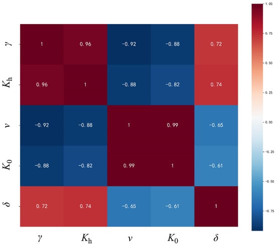
Figure 7.
Correlation analysis of several geological parameters.
3.3. Model Establishment
The principles of MLR, KNN, SVR, CART, and BPNN have been introduced in detail in Section 2, and an optimization algorithm–genetic algorithm was also described. For the first four algorithms, on the one hand, these algorithms are relatively simple and have fewer hyperparameters. In this regard, this paper used python language for code programming, and the sk-learn library was imported to quickly build the prediction model. The input parameters will follow the various strategies presented in Section 2.7. In terms of hyperparameters, the MLR model had no hyperparameters, and for the KNN, the default value of the model was k = 5. The quality of the SVR model was mainly related to the kernel function. In this paper, ‘rbf’ kernel function is selected to effectively deal with nonlinear regression problems. The main hyperparameter of CART was the depth of the tree. The greater the depth, the more branches of the tree and the more features of the extracted data, which can make the prediction result of the model approximately close to the real value. However, on the other hand, this also increases the complexity of the model, which will reduce its generality, and lead to the phenomenon of overfitting of the model. In this regard, this paper will calculate the model loss for each depth of the decision tree, and the optimal depth will be used as a hyperparameter for latter CART model.
For the BPNN, as an intelligent algorithm, it has higher operability and more hyperparameters. Both the number of network layers and the number of nodes per layer have a great impact on the network accuracy. In addition, the choice of activation function between layers is also a big task. The Kereas library provides us with many activation functions—such as ‘relu’, ‘tanh’, ‘elu’, etc.—which can better analyze the nonlinear relationship of data in the model. Optimizers—such as ‘adam’ and ’sgd’—can speed up model convergence and train the best model better and faster. In addition, batch size is also a hyperparameter worth considering for the size of the batch data read each time during model training will affect the learning rate. If it is too large, the model cannot take into account some details, and if it is too small, it is easy to reduce the generalization ability of the model. In this way, the number of hyperparameter combinations involved in building a BPNN model is huge. In this paper, we introduce a genetic algorithm accordingly. By geneticizing each hyperparameter, each hyperparameter combination as a gene. The model of survival of the fittest is inherited, and finally, the algorithm can help us select the optimal combination of hyperparameters, which can make our model best adapt to our data situation. In this regard, we first set up the gene pool of the genetic algorithm. For the number of layers of the model, we set up four kinds of genes—1, 2, 3, and 4. For the neurons of each layer, we will select from the list [10, 11, 12, 14, 15, 16, 18, 19, 20, 22, 25, 28, 32, 45, 64, 100, 128]. In terms of activation function, ‘relu’, ‘elu’, ‘tanh’, ‘sigmoid’, ‘hard_sigmoid’, ‘softplus’, and ‘linear’ will be chosen as gene library. As for the optimizer, we provide the list ‘adam’, ‘sgd’, ‘adagrad’, ‘adadelta’, ‘adamax’, and ‘nadam’. The batch size is selected from the list [10, 12, 16, 32, 48, 64, 128].
By using the genetic algorithm, repeated combining hyperparameters will be avoided, so the speed and efficiency of our model building will be improved.
3.4. Assessment Index
In order to evaluate the several prediction models proposed in this paper effectively, performance evaluation is indispensable. In this study, four commonly used indicators are selected to effectively evaluate the five proposed machine learning models. They are: mean absolute error (MAE), mean square error (MSE), root mean square error (RMSE), and coefficient of determination (R2), and can be defined by Equations (15)–(18):
where, y is the actual advance rate value; p is the predicted value of AR; n is the ring number; y is the average value of the AR of each ring; MAE, MSE, and RMSE are used to calculate the loss between the true value and the predicted value. The smaller they are, the better the model is, and R2 reflects the degree of matching between the predicted value and the true value, and its target value is close to 1.
4. Results and Discussion
In this paper, five proposed machine learning models were applied to five strategies for comparative learning. In order to better display the optimal results, firstly, the best machine learning model for each strategy was selected, and then on this basis, each strategy would be compared to choose the best strategy for AR prediction in mixed ground.
4.1. Best BPNN Framework for Each Strategy
First of all, for the neural network model, they were optimized according to five strategies by the genetic algorithm separately. The optimization process is shown in Figure 2. Through GA, the population was continuously inherited and evolved to find the optimal combination of genes from the gene pool. Each gene represented a hyperparameter, and the combination of hyperparameters was used to construct the final neural network framework, which would avoid repeating invalid attempts and effectively reduce the time spent on model building. After inputting the data into the genetic algorithm model, the hyperparameters of the BPNN were obtained. Then, the best network structure for each strategy was achieved, as shown in Table 4.
Table 4.
Neural network structure of each strategy.
Based on the neural network architecture obtained by genetic algorithm optimization, we used the TensorFlow framework to build a BPNN. Take Strategy A as an example. Figure 8 shows the change in MSE error between the training set and the test set during the training process. At the beginning, the error decreased very quickly. The log coordinates were chosen to make the graph data more uniform. It can be seen that—with the continuous progress of the training epochs—the error of the training set decreased rapidly at first, and then gradually slowed down, while for the test set, after it fell to a certain extent, it began to rise. In order to show the rising trend of loss in the test set more clearly, we drew 50–500 epochs (the shaded part in Figure 8a) as Figure 8b, it can be seen that the model reached the lowest point of loss around the 220th epoch, and then training the model would only infinitely reduce the training set error, but could not optimize the test set, which mainly resulted from the overfitting of the model. To avoid this phenomenon, the training needed to be terminated when the error of the test set reached the minimum. This method can improve the generalization ability of the model.
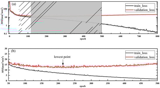
Figure 8.
BPNN model training process of Strategy A. (a) the MSE values in total process. (b) the MSE values in 50–500 epochs.
4.2. Model Assessment
Next, this paper comprehensive compared the application of the optimal structure of the five proposed machine learning algorithms in advance rate prediction to determine the most effective algorithm. The evaluation method still adopted the indicators mentioned in Section 3.4. The values of the performance indices for the proposed MLR, KNN, SVR, CART, and BPNN models were calculated, as presented in Figure 9 and Table 5. The results were divided into a training set and a test set, since the quality of a model was judged by its effect on the test set to a greater extent. Only the data obtained from the test set was used in Figure 9.
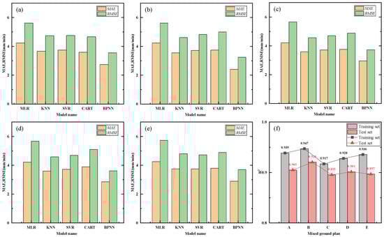
Figure 9.
Evaluation result: (a) five models’ MAE and RMSE values in Strategy A; (b) five models’ MAE and RMSE values in Strategy B; (c) five models’ MAE and RMSE values in Strategy C; (d) five models’ MAE and RMSE values in Strategy D; (e) five models’ MAE and RMSE values in Strategy E; (f) BPNN models’ R2 values in each strategy.
Table 5.
MAE and RMSE values of each model in the five strategies.
It can be seen from the Figure 9a that the errors of regression prediction implemented by different algorithms were different. Both MAE and RMSE showed significant advantages of BPNN. Figure 9b–e shows Strategy B, Strategy C, Strategy D, and Strategy E performance of each model, we can also conclude that BPNN had achieved the smallest error fitting prediction. For the other four models, there were also slight differences for different strategies. The second-best prediction model for Strategy B, C, and D was the KNN algorithm, while that for Strategy A and E was CART and SVR respectively. It can be seen that each algorithm would have its own field and can achieve good results. At the same time, it can be also seen that—among the five strategies—the model error obtained by MLR was the largest, which also showed that the advance rate of the shield machine was not a simple linear relationship with the shield parameters and geological parameters, but a more complex nonlinear relationship, so it was difficult to achieve an ideal fitting effect by using linear regression.
4.3. Optimum Solution for Mixed Ground
As shown in Figure 9a–e, the parameter-optimized BPNN achieved the minimum error prediction in all five strategies, but due to the fact that the data processing scheme was different in each strategy, which can be seen in Section 2.7, it was necessary to further analyze the advance rate prediction model of the shield tunneling that was suitable for mixed ground.
In Figure 9f, the prediction models trained by BPNN in each strategy were horizontally analyzed, and their R2 were compared. The closer R2 is to 1, the more accurate the model’s prediction is. For the data of the training set, we can easily find that Strategy B achieved the best results both in the training set and the test set. For the training set, the accuracy of Strategy B was 1% higher than that of the second-best strategy, and for the test set, the accuracy of Strategy B was 2% higher than that of the second-best strategy, while Strategy A’s R2 value was only 0.905, far less than the 0.920 of Strategy B. For a prediction model, if it can achieve high prediction accuracy on the training set, indicating that the model learns the data of the training set very thoroughly, but for the data of the test set that it has never been exposed to, it can better reflect the generalization of the model. The high accuracy of the training set with the low accuracy of the test set reflects the overfitting of the model. Fortunately, the errors obtained between the training set and the test set of the model in the five strategies were not much different, indicating that the models were well trained and there was no overfitting.
By analyzing the reasons, it can be found that the difference between Strategy B and Strategy A was that Strategy B introduced the composite ratio parameter p. This reflected the proportion of different strata in the mixed ground, and the difference between Strategy B, Strategy C, Strategy D, and Strategy E lied in the way they each deal with the geological parameters of the upper and lower layer. Strategy B took both of them as inputs to the model, while the other strategies comprehensively considered the geological parameters of the upper and lower layers. Although different comprehensive methods were used, they were not the actual relationship between them and the advance rate. The connection between them and the advance rate should be a more complex nonlinear relationship, and this relationship, benefitting from of the power of BPNN, was obtained by Strategy B, so it can achieve a better test accuracy.
4.4. AR Prediction Results
Figure 10 shows the predicted value and the measured value of the advance rate of the 238 rings’ data. It can be seen that they were relatively close. Because the selection of the test set was random, the geographic space of these data was not continuous. However, through the display of the test set data, including the regression graph shown in Figure 11, the predicted value had a strong linear relationship with the true value. That was, within the allowable range of error, it can be considered that they satisfied a linear relationship. It can be concluded that the accuracy of the neural network model was quite reliable for predicting the advance rate, compared with traditional empirical formulas or numerical models.
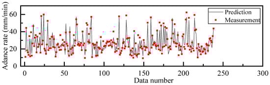
Figure 10.
Comparison of AR obtained with the BPNN model and actual measured value on test set.
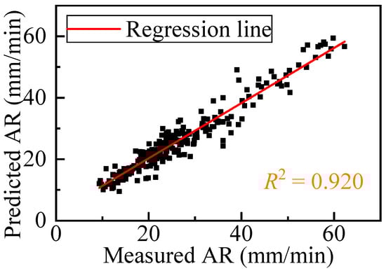
Figure 11.
Predicted and actual AR values by the BPNN model for the test datasets.
In addition, Figure 12 shows the predicted value and measured value of the advance rate of the total 1188 rings in the whole shield tunneling propulsion process. Due to the complex and changeable geological conditions, it can be seen that the advance rate fluctuates greatly. Whether it was from the data error of a single point or the overall trend, the results obtained by the neural network were still very accurate, which also confirmed the reliability of Strategy B for the prediction of the advance rate in mixed ground.
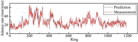
Figure 12.
Performance of BPNN on all data.
5. Conclusions
This paper proposed an optimized BPNN model using genetic algorithm. Four other machine learning methods were used for comparison. In view of the fact that there is little research on the prediction of the tunneling parameters of the shield tunneling in the mixed ground, this paper proposed five strategies to deal with the multi-geological parameters of the mixed ground, selecting different forms of geological parameters for prediction separately. Two indicators MAE and RMSE were used to evaluate the performance of different models. In the strategy selection, the statistical R2 was used to evaluate the pros and cons of each strategy. Finally, the field data of a section of Nanjing Rail Transit S6 line were used for verification. The main conclusions from this study are as follows:
- It was feasible to combine genetic algorithm with back-propagation neural network. By optimizing the combination of hyperparameters, it can quickly find the best network structure and help the neural network achieve the best prediction effect.
- Compared with the other four models, the BPNN model provided the best performances. With the help of genetic algorithm, the optimal combination of model hyperparameters can be found in a short time.
- Shield tunneling parameter data of 1188 rings, combined with the geological parameter data obtained from the geological exploration, were used to train and test the models. Four error indicators were employed and the results showed that the model obtained by MLR had the worst fitting effect, while BPNN had a strong learning ability. The performance of the BPNN model was significantly better than the other four models, so the BPNN model was determined as the optimal advance rate prediction model in this study.
- Five strategies were proposed to solve the mixed ground engineering puzzle. The only difference between them was the treatment of the geological parameters of the mixed ground. After comparison, the best prediction was achieved by Strategy B, which took the geological parameters of the upper and lower layer as input, and introduced the parameter of the composite ratio at the same time. This provided a reference for the selection of input parameters for our subsequent model establishment of shield tunneling parameter prediction in mixed ground.
- A sample of 238 rings of data was randomly selected to test the performance of the model. The results showed that the BPNN obtained in scheme B can effectively predict the AR, and the R2 reached 0.920, which can be used for prediction and control of construction tunneling parameters.
The models and conclusions in this study present some references for the shied tunneling parameters prediction in the mixed ground. However, there are still some key steps that are worth continuing to study, and the accuracy of the prediction of the AR needs to be further improved. Furthermore, since the relationship between advance rate and the geological parameters is a more complex nonlinear relationship, other models—such as the LSTM model—can also be used for further analysis and comparison. Therefore, further study needs to be conducted to find a more suitable solution.
Author Contributions
Conceptualization, X.F. and Q.G.; Methodology, X.F. and Y.W.; Software, X.F.; Resources, Q.G.; Data curation, Y.W. and H.L.; Writing—original draft preparation, X.F.; Writing—review and editing, Y.W. and Y.Z.; Funding acquisition, Q.G. All authors have read and agreed to the published version of the manuscript.
Funding
The authors are grateful for the support from the National Natural Science Foundation of China (51978523).
Institutional Review Board Statement
Not applicable.
Informed Consent Statement
Not applicable.
Data Availability Statement
The data used to support the findings of this study are available from the corresponding author upon request.
Conflicts of Interest
The authors declare no conflict of interest.
References
- Zhang, Q.; Su, C.; Qin, Q.; Cai, Z.; Hou, Z.; Kang, Y. Modeling and prediction for the thrust on EPB TBMs under different geological conditions by considering mechanical decoupling. Sci. China Technol. Sci. 2016, 59, 1428–1434. [Google Scholar] [CrossRef]
- Gong, Q.; Yin, L.; Ma, H.; Zhao, J. TBM Tunnelling under adverse geological conditions: An overview. Tunn. Undergr. Space Technol. 2016, 57, 4–17. [Google Scholar] [CrossRef]
- Ren, D.J.; Shen, J.S.; Chai, J.C.; Zhou, A. Analysis of disc cutter failure in shield tunnelling using 3D circular cutting theory. Eng. Fail. Anal. 2018, 90, 23–35. [Google Scholar] [CrossRef]
- Rehman, H.; Naji, A.M.; Nam, K.; Ahmad, S.; Muhammad, K.; Yoo, H.-K. Impact of Construction Method and Ground Composition on Headrace Tunnel Stability in the Neelum–Jhelum Hydroelectric Project: A Case Study Review from Pakistan. Appl. Sci. 2021, 11, 1655. [Google Scholar] [CrossRef]
- Wang, Q.; Xie, X.; Shahrour, I. Deep learning model for shield tunneling advance rate prediction in mixed ground condition considering past operations. IEEE Access 2020, 8, 215310–215326. [Google Scholar] [CrossRef]
- Lin, S.S.; Zhang, N.; Zhou, A.; Shen, S.L. Time-series prediction of shield movement performance during tunneling based on hybrid model. Tunn. Undergr. Space Technol. 2022, 119, 104245. [Google Scholar] [CrossRef]
- Rostami, J. Development of a Force Estimation Model for Rock Fragmentation with Disc Cutters through Theoretical Modeling and Physical Measurement of Crushed Zone Pressure. Ph.D. Thesis, Colorado School of Mines, Golden, CO, USA, 1997. [Google Scholar]
- Shi, H.; Yang, H.; Gong, G.; Wang, L. Determination of the cutterhead torque for EPB shield tunneling machine. Autom. Constr. 2011, 20, 1087–1095. [Google Scholar] [CrossRef]
- Kim, K.; Kim, J.; Ryu, H.; Rehman, H.; Jafri, T.H.; Yoo, H.; Ha, S. Estimation Method for TBM Cutterhead Drive Design Based on Full-Scale Tunneling Tests for Application in Utility Tunnels. Appl. Sci. 2020, 10, 5187. [Google Scholar] [CrossRef]
- Zhao, Y.; Gong, Q.; Tian, Z.; Zhou, S.; Jiang, H. Torque fluctuation analysis and penetration prediction of EPB TBM in rock–soil interface mixed ground. Tunn. Undergr. Space Technol. 2019, 91, 103002. [Google Scholar] [CrossRef]
- Alsahly, A.; Stascheit, J.; Meschke, G. Advanced finite element modeling of excavation and advancement processes in mechanized tunneling. Adv. Eng. Softw. 2016, 100, 198–214. [Google Scholar] [CrossRef]
- Lee, H.; Choi, H.; Choi, S.W.; Chang, S.H.; Kang, T.H.; Lee, C. Numerical simulation of EPB shield tunnelling with TBM operational condition control using coupled DEM–FDM. Appl. Sci. 2021, 11, 2551. [Google Scholar] [CrossRef]
- Sheil, B.B.; Suryasentana, S.K.; Mooney, M.A.; Zhu, H. Machine learning to inform tunnelling operations: Recent advances and future trends. Proc. Inst. Civ. Eng. Smart Infrastruct. Constr. 2020, 173, 74–95. [Google Scholar] [CrossRef]
- Yagiz, S.; Gokceoglu, C.; Sezer, E.; Iplikci, S. Application of two non-linear prediction tools to the estimation of tunnel boring machine performance. Eng. Appl. Artif. Intell. 2009, 22, 808–814. [Google Scholar] [CrossRef]
- Mobarra, Y.; Hajian, A.; Rahgozar, M. Application of artificial neural networks to the prediction of TBM penetration rate in TBM-driven golab water transfer tunnel. In Proceedings of the International Conference on Civil Engineering Architecture & Urban Sustainable Development, Tabriz, Iran, 27–28 November 2013; Volume 27. [Google Scholar]
- Salimi, A.; Moormann, C.; Singh, T.; Jain, P. TBM Performance Prediction in rock tunneling using various artificial intelligence algorithms. In Proceedings of the 11th Iranian and 2nd Regional Tunnelling Conference “Tunnels and the Future”, Tehran, Iran, 2–5 November 2015. [Google Scholar]
- Koopialipoor, M.; Tootoonchi, H.; Jahed Armaghani, D.; Tonnizam Mohamad, E.; Hedayat, A. Application of deep neural networks in predicting the penetration rate of tunnel boring machines. Bull. Eng. Geol. Environ. 2019, 78, 6347–6360. [Google Scholar] [CrossRef]
- Chen, R.; Zhang, P.; Kang, X.; Zhong, Z.; Liu, Y.; Wu, H. Prediction of maximum surface settlement caused by earth pressure balance (EPB) shield tunneling with ANN Methods. Soils Found. 2019, 59, 284–295. [Google Scholar] [CrossRef]
- Gao, X.; Shi, M.; Song, X.; Zhang, C.; Zhang, H. Recurrent neural networks for real-time prediction of TBM operating parameters. Autom. Constr. 2019, 98, 225–235. [Google Scholar] [CrossRef]
- Chen, H.; Xiao, C.; Yao, Z.; Jiang, H.; Zhang, T.; Guan, Y. Prediction of TBM Tunneling Parameters through an LSTM neural network. In Proceedings of the 2019 IEEE International Conference on Robotics and Biomimetics (ROBIO), Dali, China, 6–8 December 2019; pp. 702–707. [Google Scholar]
- Tóth, Á.; Gong, Q.; Zhao, J. Case studies of TBM tunneling performance in rock–soil interface mixed Ground. Tunn. Undergr. Space Technol. 2013, 38, 140–150. [Google Scholar] [CrossRef]
- Zhou, X.; Zhai, S. Estimation of the cutterhead torque for earth pressure balance TBM under mixed-face conditions. Tunn. Undergr. Space Technol. 2018, 74, 217–229. [Google Scholar] [CrossRef]
- Wu, X.; Kumar, V.; Quinlan, J.R.; Ghosh, J.; Yang, Q.; Motoda, H.; McLachlan, G.J.; Ng, A.; Liu, B.; Yu, P.S.; et al. Top 10 algorithms in data mining. Knowl. Inf. Syst. 2008, 14, 1–37. [Google Scholar] [CrossRef] [Green Version]
- Cortes, C.; Vapnik, V. Support-vector networks. Mach. Learn. 1995, 20, 273–297. [Google Scholar] [CrossRef]
- Smola, A.J.; Schölkopf, B. A tutorial on support vector regression. Stat. Comput. 2004, 14, 199–222. [Google Scholar] [CrossRef] [Green Version]
- Rumelhart, D.E.; Hinton, G.E.; Williams, R.J. Learning representations by back-propagating errors. Nature 1986, 323, 533–536. [Google Scholar] [CrossRef]
- Zhou, J.; Bejarbaneh, B.Y.; Armaghani, D.J.; Tahir, M.M. Forecasting of TBM advance rate in hard rock condition based on artificial neural network and genetic programming techniques. Bull. Eng. Geol. Environ. 2020, 79, 2069–2084. [Google Scholar] [CrossRef]
- Sampson, J.R. Adaptation in natural and artificial systems (John H. Holland). SIAM Rev. 1976, 18, 529–530. [Google Scholar] [CrossRef]
- Mirjalili, S. Genetic algorithm. In Evolutionary Algorithms and Neural Networks; Springer: Cham, Switzerland, 2019; pp. 43–55. [Google Scholar] [CrossRef]
- Whitley, D. A Genetic algorithm tutorial. Stat. Comput. 1994, 4, 65–85. [Google Scholar] [CrossRef]
- Xu, H.; Zhou, J.; Asteris, P.G.; Armaghani, D.J.; Tahir, M.M. Supervised machine learning techniques to the prediction of tunnel boring machine penetration rate. Appl. Sci. 2019, 9, 3715. [Google Scholar] [CrossRef] [Green Version]
- Mokhtari, S.; Mooney, M.A. Predicting EPBM advance rate performance using support vector regression modeling. Tunn. Undergr. Space Technol. 2020, 104, 103520. [Google Scholar] [CrossRef]
Publisher’s Note: MDPI stays neutral with regard to jurisdictional claims in published maps and institutional affiliations. |
© 2022 by the authors. Licensee MDPI, Basel, Switzerland. This article is an open access article distributed under the terms and conditions of the Creative Commons Attribution (CC BY) license (https://creativecommons.org/licenses/by/4.0/).