Featured Application
This research is based on a self-developed wearable lower limb exoskeleton system, which can identify a variety of motion modes and conversion modes through the collected lower limb motion information. The significance of this research is to propose a locomotion mode recognition algorithm, which can recognize the motion pattern quickly and accurately to the benefit of the control of an exoskeleton robot.
Abstract
This paper proposes a hierarchical support vector machine recognition algorithm based on a finite state machine (FSM-HSVM) to accurately and reliably recognize the locomotion mode recognition of an exoskeleton robot. As input signals, this method utilizes the angle information of the hip joint and knee joint collected by inertial sensing units (IMUs) on the thighs and shanks of the exoskeleton and the plantar pressure information collected by force sensitive resistors (FSRs) are used as input signals. This method establishes a framework for mode transition by combining the finite state machine (FSM) with the common locomotion modes. The hierarchical support vector machine (HSVM) recognition model is then tightly integrated with the mode transition framework to recognize five typical locomotion modes and eight locomotion mode transitions in real-time. The algorithm not only reduces the abrupt change in the recognition of locomotion mode, but also significantly improves the recognition efficiency. To evaluate recognition performance, separate experiments are conducted on six subjects. According to the results, the average accuracy of all motion modes is 97.106% ± 0.955%, and the average recognition delay rate is only 25.017% ± 6.074%. This method has the benefits of a small calculation amount and high recognition efficiency, and it can be applied extensively in the field of robotics.
1. Introduction
For the exoskeleton to assist human movement in the exoskeleton robot system [1], it is necessary to precisely control the exoskeleton robot so that it follows the human’s movements, and ultimately achieves human–machine coordinated movement. In general, the control strategies for various locomotion modes are distinct. Incorrect application of the control strategy may result in the robot impeding or even harming the human movement. Therefore, accurate and real-time recognition of locomotion modes is the foundation of exoskeleton control, which is of great significance [2,3,4].
In recent years, scholars domestically and internationally have conducted extensive research on locomotion pattern recognition based on the signals measured by mechanical sensors and bioelectric signals such as electromyography (EMG), which has yielded numerous results [5,6,7,8]. Among them, EMG primarily measures the electrical signal generated by muscle cells 100 ms before muscle activity [9], which is predictive in advance. Deepak et al. [10] proposed that classification could be performed using the discriminant function or if–else rule set, the learning algorithm derived from the training example, and a priori knowledge to reduce the average classification error to 11%. According to the non-stationary characteristics of leg EMG signals during movement, a new phase-related EMG PR strategy was proposed to classify the user’s movement patterns; the average classification errors in the four defined phases using ten electrodes placed over the muscles above the knee were 12.4%, 6.0%, 7.5%, and 5.2%, respectively [11]. However, the electrode for EMG signal acquisition had to be affixed to the skin surface of wearer, which was not only inconvenient in practice but also disrupted by perspiration [12]. This method is simple and straightforward to realize the benefits of low interference [13], as the mechanical sensor is primarily on the exoskeleton machinery. Specifically, the multi-source information fusion technology that integrates various types of sensors can obtain more information than a single type of sensor, thereby enhancing recognition performance [14,15].
Feng et al. [16] proposed a motion patterns recognition method based on convolutional neural network (CNN) and strain gauge signals, identifying three motion patterns of flat, ascending terrain and descending terrains with a 92.06% overall recognition accuracy. In the literature, Liu et al. developed a pure mechanical sensor architecture consisting of accelerometers, gyroscopes and pressure insole sensors [17]. The Cartesian product of five terrain types and three walking speeds defined 15 sample sets of motion intention. The measured real-time data were used to calculate the inter-observer reliability (ICC) with the template data and the Dempster–Shafer (D–S) data fusion theory, and the hidden Markov model (HMM) was used to recognize the real-time motion state with an average accuracy of 95.8% based on the reference to the previous step. However, there was neither continuous processing of motion data, nor mutual recognition of terrain pattern conversions. Long et al. used particle swarm optimization (PSO) to optimize support vector machine (SVM) for classification and identification based on plantar pressure signal and leg posture signal, with a 96.00% ± 2.45% accuracy rate. Following this, the majority voting algorithm (MVA) was utilized for post-processing, and the recognition accuracy reached 98.35% ± 1.65% [18]. The paper [19] proposed a support vector machine model based on simulated annealing algorithm to identify three distinct motion modes. It then used a finite state machine to limit state transition for post-processing to improve the overall performance of the system, with recognition accuracy reaching 97.47% ± 1.16%. Wang et al. used a rule-based classification algorithm to achieve real-time recognition of the three most common motion modes of flat walking, stair climbing and stair descending. The average accuracy of recognition reached 98.2%, and the average delay in recognition for all conversions was slightly less than one step [20]. Regrettably, these studies did not conduct a more in-depth examination of the miscalculation in the stable locomotion mode and the computational efficiency.
Various algorithms, such as Latent Dirichlet Allocation (LDA), Bayesian algorithm network, neural network, support vector machine (SVM), and so on, are commonly used to solve classification problems. The SVM model is a two-classification model; for multi-classification problems, additional improvements [21,22,23,24] are required. Commonly used techniques include one to one (OVO) [21], one to rest (OVR) [22], directed acyclic graph SVMs (DAG SVMs) [23], hierarchical support vector machines (HSVM) [24], and others. Undoubtedly, these strategies will increase the amount of computation to varying degrees, resulting in a decrease in algorithm efficiency. Reference [25] proposed a design method of hierarchical support vector machine multi-class classifier based on the inter-class separability. Experimental results indicated that this method increased the classification accuracy and accelerated the classification speed. We propose a hierarchical support vector machine algorithm based on finite state machines (FSM-HSVM). The algorithm combines the finite state machine with common locomotion modes to create a mode framework, then combines this framework with the hierarchical support vector machine recognition model. Hip angle, knee angle and plantar pressure data collected by IMUs and FSRs are preprocessed as a training signal input. Then, for real-time recognition, one or all sub-classifiers in the HSVM model are invoked in the FSM framework. To validate the efficacy and precision of the proposed algorithm, a large number of experiments are conducted under five typical motion modes and eight locomotion mode transitions.
The organizational structure of this paper is as follows. Section 2 first introduces the structure, data acquisition system and data source of exoskeleton robot, then introduces HSVM theory and FSM theory, as well as the process of recognition algorithm for motion pattern recognition, and finally introduces the evaluation index of algorithm performance. Section 3 and Section 4, respectively, present the experimental results and discussion. The conclusion is presented in Section 5.
2. Materials and Methods
2.1. Exoskeleton Structure and Data Collection
The Beijing Institute of Technology developed a new type of lower limb exoskeleton robot powered by motor drive with a maximum load capacity of 60 kg. This exoskeleton robot mechanism closely resembles the structure of human lower extremity. The length of exoskeleton rods such as the thigh and lower leg can be adjusted based on the subject’s body shape to accommodate different subjects. Instead of focusing on a ball-and-socket structure, the BIT exoskeleton designs the three degrees of freedom at the hip joint independently to reduce interference between the lower limb exoskeleton and human movement and to improve wearing comfort. Additionally, the knee joint is designed as a hinged structure hinged around the coronal axis, which is simpler and more reliable. After rigorous research and demonstration, the structure of the lower limb exoskeleton robot of BIT can meet the design requirements. The total mass is lighter and more flexible compared to the hydraulic exoskeleton [26]. Key exoskeleton components incorporate elastic units and limit devices for the comfort and safety of human wear. The mechanical system of the exoskeleton consists of a bionic back frame, hip assist mechanism, knee assist mechanism, and lower limb support mechanism. The back frame adopts the split design of human bionics and conforms well to the human body, allowing it to be worn by personnel of a specific height and body shape. The hip assist mechanism uses a direct drive motor to assist the body in sagittal flexion, while the knee assist mechanism uses a rope wheel structure to assist the knee joint. Not only should the lower limb support mechanism connect to other mechanisms as a support, but it should also be responsible for transmitting gravity to the ground.
As shown in Figure 1, the movement data of lower limbs are collected by plantar pressure detection system and inertial measurement units. After collecting the motion information of each component, it is transmitted via the RS485 bus to the arm main control computer to complete the exoskeleton robot’s driving and control. The data transmission frequency is 100 Hz, and the core chip utilizes a Samsung S5P6818 development board (ARM Cortex-A53 architecture), 2 GB RAM, 16 GB EMMC. The plantar pressure detection system records stress data using four force sensitive resistors (LOSON LSH-10) placed in the sole and heel of shoes. Each force sensitive resistor (FSR) has a 200 kg measurement limit and an overall accuracy of 0.5% full scale (FS). The inertial measurement units (IMU JY901) are positioned in the middle of the exoskeleton’s thighs and shanks to collect lower limb motion data. IMU JY901 could read the three-axis acceleration, three-axis angular velocity, three-axis magnetic field and other original sensor data, then calculate the three-axis attitude angle in real-time using the Kalman filter algorithm and the dynamic decoupling algorithm. As human walking is parallel to the sagittal plane, only the Z-axis rotation angle is required. The measurement range is −180~180°, and the dynamic angle resolution is 0.1°. The hip joint is the angle between the vertical and the thigh directions, whereas the angle of the knee joint is the angle between the thigh and the shank.
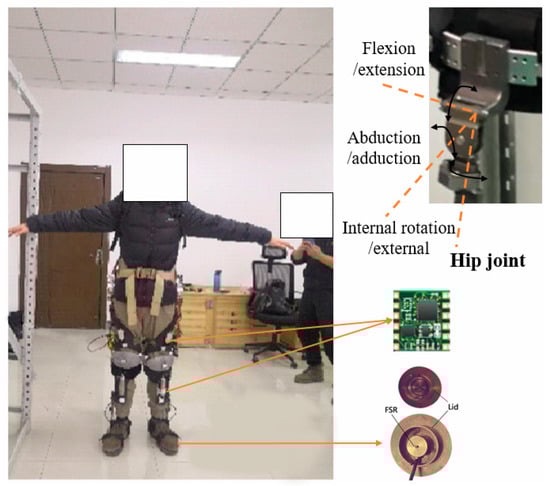
Figure 1.
The lower extremity exoskeleton robot of BIT.
2.2. Data Source
The following is a unified definition of the concepts related to locomotion mode to facilitate discussion. The human body’s locomotion modes fall into two categories: stable locomotion mode and locomotion mode transition. Stable locomotion mode refers to continuous motion in a single locomotion mode, whereas locomotion mode transition refers to the rapid transition from one locomotion mode to another during motion. The transition time of the locomotion mode is defined uniformly as the moment when the leading foot of the previous mode leaves the ground, and the cycle from this time until the next time this foot first leaves the ground in the next mode is known as the locomotion mode transition period.
A total of five subjects volunteered to participate in this experiment, and the height of these subjects was 1.60~1.80 m and the weight was 60~80 kg. Before the experiment, all participants were informed of all experimental procedures and had no diseases. Before the experiment, the connection between each structural member and the exoskeleton’s information acquisition system was checked to ensure that the sensor is calibrated and in a standard state. When a subject is wearing an exoskeleton, the length of the exoskeleton rod is adjusted based on the subject’s feelings. Then the subjects walked adaptively for approximately one minute, after which they continued to fine-tune their gait to maximize human comfort and flexibility. Each subject wore an exoskeleton robot and conducted two types of experiments at a speed that was approximately constant and without load. The initial experiment consists of a stable mode experiment with various locomotion modes. As shown in Figure 2, the subjects walk in five modes: flat walking (FW), up the stairs (US), down the stairs (DS), up the ramp (UR) and down the ramp (DR). The staircase is 1.5 m wide, 40 cm deep, 15 cm tall, and slopes at about 26°. The ramp slope is approximately 10°, and its length is 4.5 m. Each exercise mode included five experiments for one subject, each lasting about thirty seconds. The second experiment involves the transition between various locomotion modes. Each experimenter walks from the flat ground to another locomotion mode, and from other modes to the flat ground, with a total of eight conversion modes, i.e., FWUS, USFW, FWDS, DSFW, FWUP, UPFW, FWDP, DPFW. Each transition period included five experiments on one subject lasting thirty seconds.
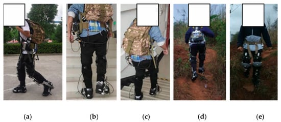
Figure 2.
Experiments of different locomotion modes. (a) Flat Walking; (b) Up the Stairs; (c) Down the Stairs; (d) Up the Ramp; (e) Down the Ramp.
Once sufficient training datasets had been obtained, the FSM-HSVM model could be trained offline. To remove noise and interference from the data collected by the acquisition system, a second-order Butterworth low-pass filter with a cutoff frequency of 5 Hz was applied. Locomotion mode recognition was performed in real-time and online. Text was used to record the recognized pattern in the processor, which was then verified and analyzed after the experiment was completed. All experiments were approved by the Beijing institute of technology’s Medical and Experimental Animal Ethics Committee, and the procedures used in this study followed the specified principles.
2.3. Feature Selection and Analysis of Motion Characteristics
When people walk with a lower limb exoskeleton robot, a large number of experimental studies [17,18,19,20,27,28] indicate that the joint angle of lower limb and plantar pressure undergo very obvious periodic changes. At the same time, the motion characteristics and change laws of various modes and gait phases are distinct, particularly the change amplitude, peak value, and change trend. These distinctions serve to distinguish between various motion modes. As a result, the hip angle, knee angle, and plantar pressure are utilized as input signals, and the resulting information combination is expressed as follows:
where are the pressure on the ball and heel of left and right legs, and are the angle of the hip and knee joints of the left and right legs. Through a comprehensive and detailed analysis of the obtained motion signals, it is possible to extract feature information with high discrimination, which lays the foundation for the later research of the recognition algorithm. Figure 3 depicts the joint angle and plantar pressure for each of the five locomotion modes.
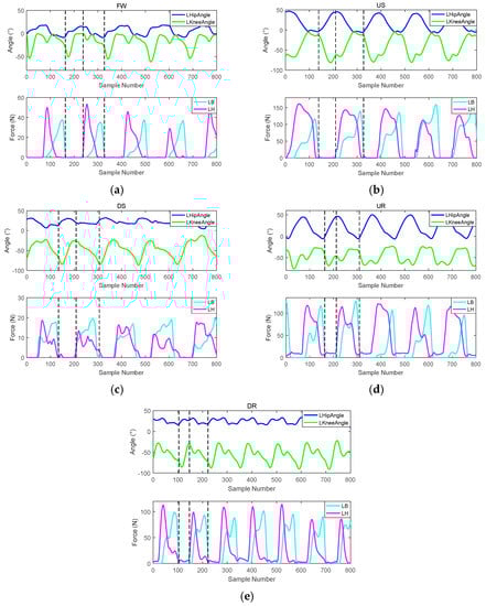
Figure 3.
The lower limb information under different locomotion modes. (a) Flat Walking; (b) Up the Stairs; (c) Down the Stairs; (d) Up the Ramp; (e) Down the Ramp.
Using walking on FW as an example, the toe off time is the beginning of a cycle. At this point, the swinging leg is behind the body, and the hip angle of the swinging leg is close to its minimum value. With an increase in the swing period, the angle of hip flexion gradually increases. The maximum angle of flexion of the hip joint was reached when the swing foot touched the ground during the support period. As the duration of support increased, the angle of hip flexion began to gradually decrease. At the conclusion of the support period, the hip angle reaches its minimum value. The knee joint’s change law of knee joint is comparable to that of the hip joint, with the exception of the time and range of extreme values. The plantar pressure clearly demonstrates that the heel contacts the bottom first, followed by the sole and the pressure change curve is very smooth without multiple extreme points.
When ascending and descending stairs and ramps, the knee angle starts to decrease from its peak at the end of the swing period, and rebounds for a time during early and late support, and then decreases. The change range and peak value of hip angle are greater than those of flat walking, and the change curve of hip angle is more sinusoidal like.
In the initial phase of descent on stairs or a ramp, the knee angle reaches the maximum and then gradually decreases. At the conclusion of the swing, the angle reaches its minimum and begins to gradually increase as the support begins. In the initial phase of support, there is a period of decline, followed by an increase to its maximum level. The hip joint’s change range and peak value are the smallest. The hip angle varies from 10° to 20°, especially when descending the ramp. This is because the hip joint is primarily responsible for maintaining body balance. Upon contact with the ground, the pressure on the heel and sole began. Specifically, there is a noticeable oscillation at the top of the stairs.
2.4. Motion Pattern Recognition Algorithm
2.4.1. Hierarchical Support Vector Machine Classifier (HSVM)
Support vector machine (SVM) [29] is a new machine learning technique founded on Vapink’s statistical learning theory (STL). The statistical learning theory implements the structural risk minimization (SRM) criterion, which minimizes sample point error and structural risk. This criterion enhances the model’s capacity for generalization, and has no restrictions on data dimension. In linear classification, the classification surface is taken at the point of greatest separation between the two sample types. Through kernel function [30], nonlinear classification problems can be into linear classification problem in high-dimensional space.
Classical SVM is limited to two classification problems, therefore, multiclassification problems require further improvement. Currently, the multi-classification SVM is primarily implemented by decomposing and reconstructing multiple binary SVMs [31]. Commonly used techniques include one to one (OVO) [21], one to rest (OVR) [22], directed acyclic graph SVMs (DAG SVMs) [23], hierarchical support vector machines (HSVM) [24], etc. These multi-classification decomposition and reconstruction methods choose various training methods and combination strategies, which determine the training and classification complexity of the classifier. For the K-classification problem, Table 1 compares the training and classification complexity of the aforementioned common multi-classification SVMs.

Table 1.
The comparison of the training and classification complexity of the multi-classification SVM.
As shown in Table 1, both OVO and DAG use a one to one approach for basic SVM training. The number of SVM sub-classifiers that must be trained is the greatest and grows exponentially as the number of K classes increases. The basic thought of OVR and HSVM is one to rest, and the number of trainers is significantly less than OVO and DAG. HSVM employs a tree structure to reduce the complexity of training and requires the training of only (K–1) SVM classifiers. OVO and OVR must traverse all trained SVMs, resulting in low overall efficiency. DAG adopts directed acyclic graph structure, and the average number of SVMs required for classification is (K–1), with a small number and high classification efficiency. Although HSVM traverses all sub-classifiers, classification efficiency is also high due to the small number of trained classifiers. To sum up, it is very clear that HSVM requires the smallest number of sub-classifiers during training and identification due to its unique tree structure, and this method has the least amount of training calculation and the highest classification efficiency. Therefore, HSVM is used to classify and identify locomotion modes in this paper. The overall structure of HSVM is comparable to that of binary tree, in which the intermediate node implements local decisions and the leaf node identifies the category. This method makes full use of a priori human behavior. In order to ensure the validity of the classification, it makes the categories within the subclasses more similar while the categories between the subclasses have clear distinctions. For HSVM to have the best generalization performance, the divisibility between the upper layer’s two subclasses must be as strong as possible [32]. Typically, the Euclidean distance between various samples in the input space is used to cluster layer by layer, so as to create a reasonable hierarchical structure. However, the Euclidean distance requires that time series data have the same length. The distance is then calculated and summed based on the points on the time axis. According to the research, the cycle length of human walking is not fixed, and the cycle length under the five different motion modes is also obviously different, leading to the fact that the time series cannot correspond one by one, so the Euclidean distance cannot be solved in this case. At this time, we can further analyze the change trend and duration of the gait cycle by using the DTW algorithm [33], and deeply analyze the similarity of data of two consecutive gait cycles based on the continuity of time. To compare the similarity of two sets of data, the distortion of their corresponding frames must be calculated. The smaller the distortion, the higher the similarity. Because the total number of frames in two segments of gait cycle data is typically different, the signal value sequence must be re-aligned in time. The algorithm for dynamic time warping can effectively solve this data comparison problem. In other words, the data sequence of the smaller total frame number is mapped to the data sequence of the larger total frame number, and the degree of distortion between the newly corresponding frames is calculated and added. Next, the complete data of one cycle under five motion modes are intercepted separately to calculate the DTW distance, as shown in Table 2, in order to investigate the similarity between various locomotion modes.
Table 2.
The DTW distance for different locomotion modes.
As shown in the table above, the most recent data groups for the five terrain types are: {FW, DR}, {US, UR}, {DS, DR}, {UR, US}, {DR, DS}. As shown in Figure 4, the five motion modes can be subdivided according to the tree structure to establish the hierarchical structure in HSVM.
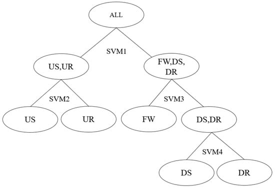
Figure 4.
Segmentation of different locomotion modes by HSVM.
As shown in Figure 3, the classification procedure involves hierarchical decision-making and gradual subdivision. First of all, five motion modes can be divided into two major categories by first classifier SVM1 according to DTW distance. The first category includes up stairs and up ramps, while the second category includes three modes: flat walking, down stairs and down ramp. Then, the classifier SVM2 is used to identify up the stairs and up the ramp, and SVM3 is used to further divide the second category into L and {DS, DR}. Ultimately, the forth classifier SVM4 is utilized to differentiate between DS and DR. So far, four classifiers have been used to separate the five motion patterns. The penalty coefficient c and the kernel function parameter will have a significant effect on the accuracy of these binary classifiers. In this paper, specific values of c and are screened using the grid method, which is easy to implement and does not require manual adjustment.
2.4.2. Finite State Machine (FSM)
Finite state machine (FSM) is a mathematical model that represents a finite number of states and the transfer and action between these states [34]. The FSM can be expressed as the following five element function group:
where represents a set of states of the finite state machine, including five common locomotion modes. is a limited set of input information, including plantar pressure and joint angle. At any given moment, the finite state machine can only be in a certain state , the finite state machine can only receive one definite input . is the state transition function. In a certain state, the finite state machine will enter a new state determined by the state transition function after a given input. is the initial state, and the finite state machine begins to receive input from this state from. is the final state set, and the finite state machine will no longer receive input after reaching the final state.
2.4.3. FSM-HSVM
The movement of human body is an action sequence consisting of continuous and sequential movements along the time axis. As long as the current motion mode is known, the following motion mode will be constrained. The human–machine movement conforms to the same as human movement, and there will be no unreasonable mode switching. For instance, if the current motion mode is ascending stairs, the locomotion mode can only be ascending stairs or walking on flat ground, and it is impossible to convert directly to going down ramp. Therefore, reasonable transformation should be taken into account when recognizing the locomotion mode, and unreasonable transformation can be eliminated immediately. This paper introduces a finite state machine to construct the exoskeleton movement mode finite state machine framework, so as to make necessary restrictions on the movement modes and their transitions.
According to actual statistics and research, there are five common motion modes: flat walking (FW), up the stairs (US), down the stairs (DS), up the ramp (UR) and down the ramp (DR). There are only eight corresponding locomotion mode transitions, namely FWUS, USFW, FWDS, DSFW, FWUR, URFW, FWDR, DRFW. The transitions between USDS and URDS modes of locomotion does not exist. When the current mode is FW, the next motion mode may be stability mode FW or four other conversion modes, i.e., US, DS, UR and DR. When the current mode is other four motion modes, the motion mode at the next time is either the same stable mode as the previous time or flat mode. Other locomotion mode transitions, such as USDS and URDS are unreasonable and do not exist in the actual environment. Figure 5 depicts the specific finite-state transition diagram of locomotion mode.
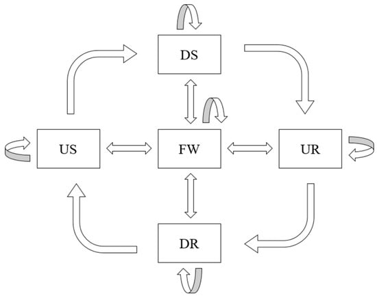
Figure 5.
Finite state machine transition diagram of locomotion modes.
Currently, the finite state machine in reference [19] is only used for mode switching post-processing and is not integrated with the recognition algorithm. This paper proposes a support vector machine algorithm based on finite state machine (FSM-HSVM). By combining the finite state machine with common locomotion modes and the HSVM recognition model, the model transformation framework is established. The algorithm can restrict mutations in the stable locomotion, and significantly enhance recognition efficiency. It can be divided into five rules for the FSM motion mode framework and HSVM recognition model fusion. The specific rules are as follows:
- If ,
- If ,
- If ,
- If ,
- If , .
According to rule 1, the next motion mode can be any of the five locomotion modes when the locomotion mode is flat walking, and the entire HSVM model must be invoked for recognition. According to rule 2, when the locomotion mode is ascending stairs, it can only continue ascending stairs or transition to walking on flat ground. Currently, only one sub-classifier SVM1 is required for recognition. Rules 3, 4 and 5 are identical to rule 2. That is, only rule 1 needs to call the whole HSVM model for recognition. Other rules need to call one sub-classifier to meet the classification requirements. The FSM-HSVM model has no more than (K–1), which is the smallest number among all multi-classification SVM methods.
2.5. Performance Evaluation
In order to evaluate the performance of the algorithm, the recognition accuracy (RA) is defined to quantify the recognition results.
where is the number of correct locomotion modes identified in the test set, is the total number of divided locomotion modes in the test set.
For a more precise analysis of gait phase recognition misclassification, the confusion matrix is constructed to quantify the error distribution.
where each element of the confusion matrix is defined as:
where is the number of events in the motion mode recognized as the motion mode during classification and recognition, is the total number of events in the locomotion mode. Thus, the diagonal elements of the confusion matrix represent the number of correct recognitions at the corresponding phase stage, whereas the non-diagonal elements represent the number of recognition errors.
In addition to the recognition accuracy, pattern recognition algorithms must typically assess whether they were detected in time. Consequently, the recognition delay rate (RD) is defined to quantify the degree of identification delay of the algorithm.
In this formula, is the moment when the locomotion mode transition is correctly recognized for the first time, is the transition moment and is the total time of a gait cycle. According to these three moments, the RD between gait mode transitions can be obtained. It is worth noting that the defined also needs to satisfy the remaining time without error determination.
In addition, the running time t of the algorithm is also an important indicator of the model performance. The time required for algorithm recognition can be used to evaluate the algorithm’s complexity and the hardware resources it requires. Since the single recognition time is extremely small and difficult to measure, the entire test set can be used for recognition, and the cumulative recognition time can be calculated.
3. Results
3.1. Experimental Results and Analysis of Locomotion Mode Recognition
In order to confirm the efficacy of the FSM-HSVM locomotion mode recognition model, the confusion matrix is used to evaluate the performance of the model using the same motion dataset. Five human subjects were required to walk at a similar speed over varied terrain. The identification motion mode label is recorded in the control software using three distinct techniques: SVM, HSVM and FSM-HSVM. As mentioned previously, the confusion matrix can be used to display the recognition accuracy. In order to study the stability and statistical law of these algorithms, it is necessary to further deal with the confusion matrix of all subjects, and the average value MEAN of each element and its corresponding standard error SEM are calculated respectively. So, the elements of the confusion matrix are expressed as MEAN ± SEM in Table 3, Table 4 and Table 5 below.
Table 3.
Confusion matrix (MEAN ± SEM) for experimental results of SVM (%).
Table 4.
Confusion matrix (MEAN ± SEM) for experimental results of HSVM (%).
Table 5.
Confusion matrix (MEAN ± SEM) for experimental results of FSM-SVM (%).
As shown in Table 3 above, the highest recognition accuracy occurs in down ramp mode with a 95.948% recognition accuracy. In flat walking, the lowest recognition accuracy is only about 83.658%. Table 4 shows the recognition accuracy for HSVM, with the highest recognition accuracy being 96.201% when going up the stairs. The recognition accuracy of flat walking remains the lowest. According to Table 5, the accuracy of motion pattern recognition exceeds 93.420%. In particular, up the stair mode has a recognition rate of 98.760%. In comparison to Table 3 and Table 4, the results demonstrate that FSM-HSVM has higher recognition accuracy. Figure 6 depicts the recognition accuracy of three algorithms. The FSM-HSVM algorithm has achieved the highest recognition accuracy across five different locomotion modes, with an average accuracy of 97.106% ± 0.955%. In addition, the flat walking mode has the lowest recognition accuracy of the three algorithms. Review the Table 3, Table 4 and Table 5 reveals that walking on flat ground is easily confused with walking down the ramp. Even with the FSM-HSVM algorithm, the probability is as high as 3.907%.
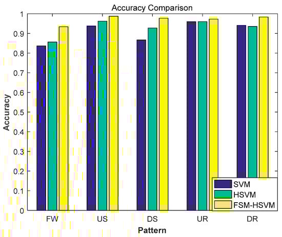
Figure 6.
Comparison of recognition rates of three algorithms.
The performance index of RRD is used to evaluate the real-time performance of the proposed recognition strategy. In this paper, Table 6 shows the RDR for the eight conversion modes. If RRD is positive, it indicates that the correct identification time is later than the actual transition time. If RDR is negative, the correct recognition time is in advance of the actual transition time. According to Table 5, the RDRs for all eight transitions between locomotion modes are positive, indicating that the correct recognition under all locomotion modes lags behind the actual conversion time. Especially for DR→FW conversion mode, the RRD can reach 53.733%. The following is UR→FW locomotion mode transition, and the delay rate is 43.067%. In other words, it can be distinguished by the middle of the whole cycle when the ramp is transitioned to flat walking. The lowest RRD is only 5.333% when FW→DS, and it indicated that the leg is correctly recognized in the early stage of swing. The average RRD is 25.017% ± 6.074% under all locomotion mode transitions. According to research, the swing period accounts for about 40% of the whole gait cycle, and the precise transition occurs roughly in the middle of the swing period.
Table 6.
DRs of locomotion mode transitions.
3.2. Algorithm Efficiency and Analysis
In order to demonstrate the complexity of the algorithm, three trained algorithm models of SVM, HSVM, and FSM-HSVM are used to identify offline the same test set that has been previously processed, and the cumulative recognition time is calculated and compared with each other; the results are depicted in Figure 7. Compared to SVM and HSVM, the algorithm proposed in this paper reduces the running time t of the algorithm by about 8 s and 3 s, respectively. In other words, the recognition efficiency of the algorithm in this paper is improved between 60% and 36%, indicating that the overall amount of calculation is small, thereby conserving a significant amount of exoskeleton hardware resources.
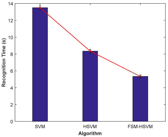
Figure 7.
Comparison of recognition time of three algorithms.
The time required for the classification and recognition of HSVM and FSM-HSVM models is discussed in detail below. Assume that is the total number of identified data samples, is the proportion of flat walking data in the total number of samples (), and the number of motion mode categories is (). The recognition time of HSVM model and FSM-HSVM are as follows.
If, . In other words, the HSVM-HSVM model degenerates into HSVM model when all data are flat walking data. If , there are no flat data in the dataset, . At this time, the recognition time is only of the recognition time of HSVM. If , the ratio between FSM-HSVM recognition time and HSVM recognition time is given by:
Obviously, the range of time ratio is: . In other words, the recognition time of the FSM-HSVM model is less than or equal to that of the conventional HSVM model. Especially when the recognition category is large or there is less flat data, the overall time will be greatly reduced compared to HSVM model, and the recognition efficiency will be significantly enhanced. In comparison to SVM and HSVM models, FSM-HSVM has the highest recognition efficiency.
4. Discussion
The experimental results show that the average recognition accuracy of FSM-HSVM for five different motion modes is 97.106% ± 0.955%, whereas the average recognition accuracies of SVM and HSVM algorithms are 90.826% ± 2.391% and 92.807% ± 1.927% respectively. In comparison with the other two algorithms, the average recognition rate increased by 6.28% and 5.036%, while the standard error decreased by 1.43% and 0.972%. Evidently, the algorithm proposed in this paper demonstrates superior recognition efficiency and recognition stability compared to SVM and HSVM. However, the results also show that the recognition accuracy of the three kinds of flat walking is the lowest, and there is a high likelihood that they are misidentified as walking down the ramp. The shortest distance, according to the DTW distance table, is between the FW and DR. It demonstrates conclusively that the similarity between the two modes is high and difficult to distinguish. This is likely due to the slope selected in this paper being only about 10°, making it virtually identical to the flat ground. At present, some good progress has been made in recognition accuracy in motion pattern recognition [18,19]. The recognition accuracy of reference [18] is as high as 98.35% ± 1.65%. However, on the premise of higher slope and easier detection, there are still obvious misjudgments in the process of stable motion pattern recognition, and the stability is weaker than that of the algorithm proposed in this paper. In reference [19], the finite state machine was used to limit the state transition for post-processing to improve the overall performance, but it was not enough for only three kinds of terrain, the common slope terrain in daily life should especially be considered. In conclusion, the proposed algorithm has better stability compared to references [18,19]. In practice, the RRDs of eight transitions between locomotion mode are extremely important. According to Table 5, we can find that the RRD is the smallest when the flat walking is converted to descending stairs, with a value of 5.333% ± 1.687%. This demonstrates that the characteristics of the transition period between flat ground and down stairs change significantly, and the algorithm is highly sensitive. The highest delay rate was 53.733% ± 9.363%, which occurred during the period from down the ramp to flat walking, and the second highest was 43.067% ± 4.107% when going from up the ramp to flat walking. This demonstrates that the feature change from ramp to ground is ambiguous, and the algorithm recognizes it only in the middle of the transition. According to that mentioned above, it is obvious that the slope gradient is small and is not different from the flat walking. The lack of prominent data collection characteristics during the transition period may be the primary cause of the high delay rate. The overall recognition delay rate is 25.017% ± 6.074%, which is significantly less than one step, indicating that the corresponding large motion mode can be recognized in the middle of swing. The conversion between these motion modes can also be accomplished through prior knowledge of the wearer or pre control, allowing the robot exoskeleton system to respond in advance, thereby ensuring system stability.
In terms of the algorithm’s recognition efficiency, the experimental results indicate that the motion time is reduced by approximately 8s and 3s compared to SVM and HSVM, respectively. Through theoretical calculation and analysis, it is also determined that the FSM-HSVM algorithm is significantly less effective than the HSVM algorithm when using SVM to solve multiclassification problems. In addition, Table 2 demonstrates that HSVM’s recognition efficiency is superior to that of other multi-classification SVM algorithms. Among the multi-classification SVM algorithms discussed in this paper, FSM-HSVM has the highest recognition efficiency. Clearly, this will significantly conserve the computing resources of exoskeleton hardware and make collaborative control of subsequent exoskeletons more feasible.
Nonetheless, there is still room for future improvement and optimization. On the one hand, walking on flat ground has a high likelihood of being interpreted as walking down the ramp, and the conversion delay rate between ramp and flat ground exceeds 40%. It is very likely to result in the miscalculation and control lag of the exoskeleton, which will affect the coordination between man and machine. In order to improve the performance of the algorithm, we will concentrate on the internal differences between the two locomotion modes, and extract higher distinguishing features for classification and recognition, thereby increasing the recognition rate and decreasing the delay rate. On the other hand, the influence of speed change under different motion modes is not taken into account, so additional research on speed adaptability is required.
5. Conclusions
In this paper, we propose a method for exoskeleton robot locomotion mode recognition in real-time. This method calculates the hip angle and knee angle using four IMUs installed on the exoskeleton as well as four plantar pressure sensors located on the sole and heel. The information is then used as input signals and imported for training into the FSM-HSVM classification algorithm model. During recognition, only one or multiple classifiers under the HSVM recognition model are required. Experiments identify five typical motion modes and eight motion mode conversions in real-time, and SVM and HSVM algorithms are used to simultaneously obtain the same input signal for training and recognition as a reference group. The experimental results indicate that that the proposed algorithm can be improved by 6.28% and 5.036% relative to SVM and HSVM, respectively, while its recognition efficiency is enhanced by approximately 60% and 36%. All transitions have an average recognition delay of less than one step. This method can be effectively applied to the recognition and control of exoskeleton intentions due to its low complexity, small amount of calculations, and high practicability.
Author Contributions
Conceptualization, Z.Q. and Q.S.; methodology, Z.Q.; investigation, Z.Q. and C.G.; resources, Z.Q., Q.S. and Y.L.; data curation, C.G.; writing—original draft preparation, Z.Q.; writing—review and editing, Z.Q., Q.S. and Y.L.; visualization, Z.Q.; supervision, Q.S.; project administration, Q.S. and Y.L.; funding acquisition, Q.S. and Y.L. All authors have read and agreed to the published version of the manuscript.
Funding
This work was supported in part by the Ministry of Science and Technology national key RD program (Grant Number: 2017YFB1300500), in part by the National Natural Science Foundation of China (Grant No.51905035), and in part by the Science and Technology Innovation Special Zone Project (Grant No. 2116312ZT00200202), and in part by the Science and Technology Innovation Special Zone Youth Project (Grant No. 2016312ZT00200203).
Institutional Review Board Statement
The study was conducted according to the guidelines of the Declaration of Helsinki, and approved by the Ethics Committee of Beijing Sport University (protocol code: 2019007H and date of approval: 22 January 2019).
Informed Consent Statement
Informed consent was obtained from all subjects involved in the study.
Data Availability Statement
The data presented in this study are available on request from the corresponding author. The data are not publicly available due to the data also forms part of an ongoing study.
Acknowledgments
The authors would like to thank all subjects who participated in the experiment.
Conflicts of Interest
The authors declare no conflict of interest.
References
- Pons, J.L. Wearable Robots: Biomechatronic Exoskeletons; Wiley: New York, NY, USA, 2008. [Google Scholar]
- Viteckova, S.; Kutilek, P.; Jirina, M. Wearable lower limb robotics: A review. Biocybern. Biomed. Eng. 2013, 33, 96–105. [Google Scholar]
- Sup, F.; Varol, H.; Mitchell, J.; Withrow, T.; Goldfarb, M. Preliminary evaluations of a self-contained anthropomorphic transfemoral prosthesis. IEEE/ASME Trans. Mechatron. 2009, 14, 667–676. [Google Scholar] [CrossRef] [PubMed] [Green Version]
- Hitt, J.; Sugar, T.; Holgate, M.; Bellmann, R.; Hollander, K. Robotic transtibial prosthesis with biomechanical energy regeneration. Ind. Robot. 2009, 36, 441–447. [Google Scholar] [CrossRef]
- Chen, B.; Zheng, E.; Wang, Q. A locomotion intent prediction system based on multi-sensor fusion. Sensors 2014, 14, 12349–12369. [Google Scholar] [CrossRef] [Green Version]
- Du-Xin, L.; Xinyu, W.; Wenbin, D.; Can, W.; Tiantian, X. Gait phase recognition for lower-limb exoskeleton with only joint angular sensors. Sensors 2016, 16, 1579. [Google Scholar]
- Young, A.J.; Simon, A.M.; Fey, N.P.; Hargrove, L.J. Intent recognition in a powered lower limb prosthesis using time history information. Ann. Biomed. Eng. 2014, 42, 631–641. [Google Scholar] [CrossRef]
- Young, A.J.; Simon, A.M.; Hargrove, L.J. A Training Method for Locomotion Mode Prediction Using Powered Lower Limb Prostheses. IEEE Trans. Neural Syst. Rehabil. Eng. 2014, 22, 671–677. [Google Scholar] [CrossRef]
- Fleischer, C.; Hommel, G. A Human-exoskeleton Interface Utilizing Electromyography. IEEE Trans. Robot. 2008, 24, 872–882. [Google Scholar] [CrossRef]
- Joshi, D.; Nakamura, B.H.; Hahn, M.E. High energy spectrogram with integrated prior knowledge for EMG-based locomotion classification. Med. Eng. Phys. 2015, 37, 518–524. [Google Scholar] [CrossRef]
- Huang, H.; Kuiken, T.A.; Lipschutz, R.D. A strategy for identifying locomotion modes using surface electromyography. IEEE Trans. BioMed. Eng. 2009, 56, 65–73. [Google Scholar] [CrossRef] [Green Version]
- Zheng, E.; Wang, L.; Wei, K.; Wang, Q. A non-contact capacitive sensing system for recognizing locomotion modes of transtibial amputees. IEEE Trans. Biomed. Eng. 2014, 61, 2911–2920. [Google Scholar] [CrossRef] [PubMed]
- Zhou, J. Research on Gait Recognition Based on Multi-Sensor Fusion. Modern Computer. 2016, 03, 40–45. [Google Scholar]
- Khaleghi, B.; Khamis, A.; Karray, F.O.; Razavi, S.N. Multisensor data fusion: A review of the state-of-the-art. Inf. Fusion 2013, 14, 28–44. [Google Scholar] [CrossRef]
- Huang, H.; Zhang, F.; Hargrove, L.; Dou, Z.; Rogers, D.; Englehart, K. Continuous locomotion mode identification for prosthetic legs based on neuromuscular-mechanical fusion. IEEE Trans. Biomed. Eng. 2011, 58, 2867–2875. [Google Scholar] [CrossRef] [Green Version]
- Feng, Y.; Chen, W.; Wang, Q. A strain gauge-based locomotion mode recognition method using convolutional neural network. Adv. Robot. 2019, 33, 254–263. [Google Scholar] [CrossRef]
- Liu, Z.J.; Lin, W.; Geng, Y.L. Intent Pattern Recognition of Lower-limb Motion Based on Mechanical Sensors. IEEE/CAA J. Autom. Sin. 2017, 4, 651660. [Google Scholar] [CrossRef]
- Long, Y.; Du, Z.J.; Wang, W.D.; Zhao, G.Y.; Xu, G.Q.; He, L.; Mao, X.W.; Dong, W. PSO-SVM Based Online Locomotion Mode Identification for Rehabilitation Robotic Exoskeletons. Sensors 2016, 16, 1408. [Google Scholar] [CrossRef] [Green Version]
- Yin, Z.; Zheng, J.; Huang, L.; Gao, Y.; Peng, H.; Yin, L. SA-SVM-Based Locomotion Pattern Recognition for Exoskeleton Robot. Appl. Sci. 2021, 11, 5573. [Google Scholar] [CrossRef]
- Wang, W.; Zhang, L.; Liu, J. A real-time walking pattern recognition method for soft knee power assist wear. Int. J. Adv. Robot. Syst. 2020, 17, 172988142092529. [Google Scholar] [CrossRef]
- Bottou, L.; Cortes, C.; Denker, J. Comparison of classifier methods: A case study in handwriting digit recognition. In Proceedings of the 12th IAPR International Conference on Pattern Recognition, Vol. 3—Conference C: Signal Processing (Cat. No.94CH3440-5), Jerusalem, Israel, 9–13 October 1994. [Google Scholar]
- Krebel, U. Pairwise classification and support vector machines. In Advances in Kernel Methods; The MIT Press: Cambridge, MA, USA, 1999; pp. 255–268. [Google Scholar]
- Platt, J.C.; Cristianini, N.; Shawe-Taylor, J. Large margin DAGs for multiclass classification. Adv. Neural Inf. Processing Syst. 2000, 12, 547–553. [Google Scholar]
- Schwenker, F. Hierarchical support vector machines for multi-class pattern recognition. In Proceedings of the International Conference on Knowledge-based Intelligent Engineering Systems & Allied Technologies, Brighton, UK, 30 August–1 September 2000. [Google Scholar]
- Zhao, H.; Rong, L.L.; Li, X. New Method of Design Hierarchical Support Vector Machine Multi-class Classifier. Appl. Res. Comput. 2006, 23, 34–37. [Google Scholar]
- Qi, Z.; Liu, Y.; Song, Q.; Zhou, N. An Improved Greedy Reduction Algorithm Based on Neighborhood Rough Set Model for Sensors Screening of Exoskeleton. IEEE Sens. J. 2021, 21, 26964–26977. [Google Scholar] [CrossRef]
- Rose, J.; Gamble, J. Human Walking; Williams and Wilkins: Baltimore, MD, USA, 1994. [Google Scholar]
- Chu, A.; Kazerooni, H.; Zoss, A. On the biomimetic design of the Berkeley lower extremity exoskeleton (BLEEX). Robot. Autom. 2006, 4, 4345–4352. [Google Scholar]
- Cortes, C.; Vapnik, V. Support-vector networks. Mach. Learn. 1995, 20, 273–297. [Google Scholar] [CrossRef]
- Hofmann, T.; Schölkopf, B.; Smola, A.J. Kernel methods in machine learning. Ann. Stat. 2008, 36, 1171–1220. [Google Scholar] [CrossRef] [Green Version]
- Hsu, C.W.; Lin, C.J. A comparison of methods for multi-class support vector machine. IEEE Trans. Neural Netw. 2002, 13, 415–425. [Google Scholar] [PubMed] [Green Version]
- Weston, J.; Watkins, C. Support vector machines for multi-class pattern recognition. In Proceedings of the European Symposium on Artificial Neural Networks (ESANN), Bruges, Belgium, 21–23 April 1999. [Google Scholar]
- Petitjean, F.; Ketterlin, A.; Gancarski, P. A global averaging method for dynamic time warping with applications to clustering. Pattern Recognit. 2011, 44, 678–693. [Google Scholar] [CrossRef]
- Zlatnik, D.; Steiner, B.; Schweitzer, G. Finite-State Control of a Trans-Femoral (TF) Prosthesis. IEEE Trans. Control. Syst. Technol. 2002, 10, 408–420. [Google Scholar] [CrossRef]
Publisher’s Note: MDPI stays neutral with regard to jurisdictional claims in published maps and institutional affiliations. |
© 2022 by the authors. Licensee MDPI, Basel, Switzerland. This article is an open access article distributed under the terms and conditions of the Creative Commons Attribution (CC BY) license (https://creativecommons.org/licenses/by/4.0/).