Early Warning of the Construction Safety Risk of a Subway Station Based on the LSSVM Optimized by QPSO

Abstract

Subway station projects are characterized by complex construction technology, complex site conditions, and being easily influenced by the surrounding environment; thus, construction safety accidents occur frequently. In order to improve the computing performance of the early risk warning system in subway station construction, a novel model based on least-squares support vector machines (LSSVM) optimized by quantum-behaved particle swarm optimization (QPSO) was proposed. First, early warning factors from five aspects (man, machine, management, material, and the environment) were selected based on accident causation theory and literature research. The data acquisition method of each risk factor was provided in detail. Then, the LSSVM with strong small sample analysis and nonlinear analysis abilities was chosen to give the early warning. To further ameliorate the early warning accuracy of the LSSVM, QPSO with a strong global retrieval ability was used to find the optimal calculation parameters of the LSSVM. Seventeen subway stations of Chengdu Metro Line 11 in China were picked as the empirical objects. The results demonstrated that the best regularization parameter was 1.742, and the best width parameter was 14.167. The number of misjudged samples of the proposed model was 1, and the early warning error rate was only 4.41%, which met the needs of engineering practice. Compared with the classic and latest methods, the proposed model was found to have a faster prediction speed and higher prediction accuracy.

1. Introduction

Due to the traffic congestion caused by the rapid increase in the urban population and prosperous economic development, major cities worldwide are actively promoting subway construction [1]. Subway station projects are the most important component of a subway system, but the majority of safety accidents of subway system construction occur in subway station projects [2]. There are many potential safety hazards in subway construction, and safety accidents caused by these risk factors are likely to cause huge human and economic losses. In addition, early risk warning is an important component of risk management that links daily risk management and emergency risk management [3]. The accurate early warning of the construction safety risk level of subway station projects could effectively improve the emergency risk management of managers, thereby ultimately reducing the losses caused by construction safety accidents to the greatest extent.

The construction content of subway station projects is complicated and includes excavation, support, the dewatering of the foundation pit, and the construction of the main and auxiliary structures of the station. In narrow and deep foundation pits, constructors of different professions operate various construction machinery. Therefore, the risk of subway station construction is characterized by many influencing factors. At present, the most commonly used method at the construction site is the checklist method [4]. Via the on-the-spot inspection of all hazard sources on the construction site, this method can directly reveal the construction safety risk status. However, this method has two serious shortcomings, namely (1) the cost is high, and the early warning efficiency is low, and (2) the result of risk early warning based on this method relies heavily on the subjective judgment of experts, so the accuracy is low.

To cope with the deficiency of the checklist method in construction risk management, a large number of scholars have put forward a variety of early warning models based on the concept of multiple linear regression [5,6,7]. These methods make full use of the multivariate heterogeneous data of the construction site and realize the low-cost and rapid early warning of the construction risk. However, they assume that there is a linear relationship between the predicted data and the risk level and therefore cannot effectively cope with the complexity of subway construction safety risks [8]; thus, the risk early warning accuracy cannot meet the needs of engineering practice.

With the vigorous development of machine learning and artificial intelligence in recent years, some scholars have applied machine learning technology to the early warning of construction safety risks. At present, the most representative models are the backpropagation neural network (BPNN) [9], the random forest (RF) [10], and the support vector machine (SVM) [11]. Related research results have shown that these new technologies could effectively improve the early warning accuracy of construction safety risks. However, the BPNN requires a huge training set to ensure the prediction results, and the data samples in engineering practice are usually small. The RF is not able to effectively cope with data with different attributes, and when the risk factors are divided into many values, the prediction results will be adversely affected. Although the SVM can sufficiently handle small sample data, it faces difficulty solving inequality constraints. When applied to the research of construction risk early warning, the SVM is characterized by some shortcomings, such as a too-large solution scale and insufficient computational performance.

The least-squares support vector machine (LSSVM) is an improved SVM, and the core of the improvement is the solution of a set of linear equations obtained by the Kuhn–Tucker condition [12]. The LSSVM reduces the solution difficulty and improves the solution speed, and it is a new application in complex problems such as power demand prediction [13], slope safety factor prediction [14], and soft soil settlement prediction [15]. In addition, in the application research of machine learning modeling, different algorithms reach different conclusions for different research problems. Therefore, it is very meaningful to introduce the LSSVM into the research of this paper.

The kernel width and the regularization parameter of the LSSVM have obvious influences on its computational performance [12,13,14]. The genetic algorithm (GA) [16] or particle swarm optimization (PSO) [17] is often used to find the optimal parameter combination. However, the GA has some shortcomings, such as low computational efficiency and premature convergence, and PSO easily falls into the trap of the local optimum because of the lack of randomness of the change of the particle position. In addition, both the GA and PSO require the preset of too many calculation parameters, which is not conducive to finding the optimal parameters of the model to be optimized. Quantum-behaved particle swarm optimization (QPSO) replaces the displacement updating formula and velocity updating formula in the traditional PSO with the wave function of quantum mechanics [18]. Because the particles in QPSO appear in all dimensions of the solution space in the form of probability, it has a better global retrieval ability than the classical meta-heuristic optimization algorithms from the aspects of the prediction and optimization of turning surface roughness [19], image segmentation optimization [20], and economic scheduling optimization [21].

According to the “no free lunch” quantification in machine learning, although many scholars have already discussed the advantages of QPSO and the LSSVM in different fields, the research of their application in the research object of this paper is still valuable.

Therefore, an early warning model of the construction safety risk of subway stations is constructed based on the LSSVM optimized by QPSO, and an empirical study on Chengdu Metro Line 11 is conducted. The contributions of this study include the following. (1) At present, most of the research results simply and roughly give the early warning index system of construction risk, lacking the relevant theoretical basis. Based on accident causation theory and the characteristics of subway station engineering, an index system is completely constructed to effectively deal with the risk complexity. To improve the engineering application value, the methods of obtaining each index are provided in detail. (2) At present, the prediction accuracy of related research cannot meet the engineering needs. Therefore, a novel early warning model integrating the computing advantage of QPSO and LSSVM is constructed to effectively deal with the strong nonlinearity of safety risks in subway station construction. (3) Different from the common simulation examples used previously, Chengdu Metro Line 11 is selected for empirical research. The findings provide new insights into the construction safety risk management of this project.

The remainder is arranged as follows. Section 2 summarizes the related research. Section 3 describes the construction of the early warning index system for the construction safety risk of subway stations and describes the methods of obtaining the index data in detail. Section 4 proposes the early warning model in detail. Section 5 describes a case analysis. Section 6 discusses the computational performance of different optimization algorithms and prediction methods to highlight the advancement of the proposed model. Finally, the research results and limitations are summarized in Section 7.

2. Related Work

To improve the efficiency of project management decision-making, Sjekavica and Radujkovic [5] used the linear regression method to construct an early warning and monitoring system for water conservancy projects. However, the data on early warning indicators (outcome factors) in that study were obtained from questionnaire surveys and expert interviews, which are not subjective. Qiu et al. [6] established a risk prediction model for oil and gas construction projects. However, although the model included the addition of grey relational analysis, it still could not effectively deal with the strong nonlinear management of the risk factors of oil and gas construction projects. Senthil and Muthukannan [7] constructed a modified historical simulation statistical method for the development, identification, and prediction of construction risk. Although the strong nonlinearity among risk factors was found to have a great influence on the prediction results, this nonlinear feature was not effectively dealt with.

Considering the strong nonlinearity of construction safety risk factors, Shen et al. [9] built a safety risk prediction model based on the BPNN. However, the research object was the entire construction industry, which lacks pertinence. Yaseen et al. [10] compared the common risk early warning methods and emphasized that artificial intelligence could sufficiently deal with the dynamics, uncertainty, and complexity of construction risks. While an RF model optimized by the GA was developed, the data were obtained from questionnaires and expert interviews. Liu et al. [11] introduced safety risk management into the design and management center of a subway station and proposed an SVM model optimized by PSO to predict the construction safety risk of subway stations. However, the prediction accuracy of the model was only 85.26%; although it was higher than other models, it still did not meet the requirements of engineering practice.

Via the powerful nonlinear modeling ability of the LSSVM, Huang et al. [13] effectively solved the problem of power demand forecasting. However, a trial algorithm was used instead of an intelligent swarm algorithm to solve the parameter combination of the LSSVM, which reduced the computational performance. Zeng et al. [14] used trial and error (TE), the gravity search algorithm (GSA), and the whale optimization algorithm (WOA) to find the best parameters of the LSSVM. Because the settlement of soft soil is a complex nonlinear system, Cui et al. [15] used the cross-validation method to get the best LSSVM model. The results showed that the selection of the control parameters had a significant impact on the predictive performance of the LSSVM. To accurately predict landslide displacement, Zhu et al. [16] proposed an LSSVM model optimized by the GA. However, the GA requires the preset of several calculation parameters, which brings a lot of trouble to the predictive work [22].

Based on QPSO, Alajmi and Almeshal [19] constructed a new prediction method for turning surface roughness. The simulation results revealed that compared with the artificial neural network (ANN) and classical meta-heuristic optimization algorithm, QPSO exhibited advantages in accuracy, robustness, and rapid convergence to the global optimum. Yang et al. [20] used QPSO to solve image segmentation and found that, compared with other optimization algorithms, QPSO improved the stability and accuracy of image segmentation. The economic dispatch problem in power systems is a typical high-dimensional nonlinear problem. Sun et al. [21] used QPSO with a powerful global retrieval ability to effectively solve this problem. The results of simulations showed that QPSO achieved better computational performance than differential evolution (DE), PSO, and the GA.

3. Early Warning Index System

3.1. Risk Identification Based on Accident Causation Theory

Accident causation theory is an accident mechanism and model extracted from the compromise of the essential causes of accidents. The system involves four basic elements, namely the unsafe behavior of men, the unsafe state of machinery, adverse effects from the environment, and the lack of management [23].

(1) Unsafe behavior of men. This mainly refers to the unsafe behavior of people, including people’s mistakes in activities, behaviors, and communication [24]. Examples include operation violations, improper emergency treatment, on-site monitoring errors, human error, malicious damage to engineering buildings or equipment by contractors, shortage of standby personnel, etc.

(2) Unsafe state of machinery. Considering the complexity of subway station engineering, in this work, the unsafe state of equipment is defined as the unsafe state of construction machinery and the unsafe state of construction materials. Inadequate investment in construction tools and equipment in subway construction will cause many problems, including outdated production equipment and incomplete or substandard safety protection facilities. These problems will reduce the disaster prevention and resistance ability of subway construction projects, which are the direct causes of many failures of safety protection facilities and poor safety protection ability.

(3) Adverse effects from the environment. Subway station engineering is generally a form of underground engineering, and its environmental impact is complex, including physical, chemical, and biological factors. The common environmental risks in subway station construction include the settlement and horizontal displacement of retaining piles, stratum subsidence and horizontal displacement, the water level of groundwater and rivers, foundation pit rebound, the geological conditions of the construction site, the construction of facilities and pipelines along the line, ground traffic and surrounding ground buildings, harmful substance injury, floods, earthquakes, fires, etc.

(4) Lack of management. The management of subway station construction includes the implementation of national guidelines, clever strategies, laws, regulations, and standards related to subway construction, the establishment of a sound safety production responsibility system, the organization of regular inspections and maintenance, and the carrying out of regular education and training on safety knowledge and skills for employees.

It should be emphasized that management mistakes cause defects in people, things, and the environment, which leads to the unsafe behaviors of subway constructors, the unsafe state of things, and an unsafe production environment, thus leading to accidents.

3.2. Early Warning Index System

Ten experts in the field of subway project management were interviewed to construct the early warning index system for the construction safety risk of subway stations. Basic information about the ten experts is reported in

Table 1. The information about the ten experts.

No.	Position	Length of Work Years	Title	Number of Subway Projects Involved
(1)	Contractor	16	Senior engineer	47
(2)	Contractor	21	Senior engineer	38
(3)	Contractor	28	Senior engineer	27
(4)	Contractor	25	Senior engineer	30
(5)	Contractor	10	Senior engineer	35
(6)	Design	35	Senior engineer	147
(7)	Design	38	Senior engineer	205
(8)	Government	12	Senior engineer	7
(9)	Government	5	Intermediate engineer	5
(10)	Academy	35	Professor	16

.

The ten experts who participated in the interview were all from units related to subway station projects, which indicates they had a good professional background. Their average number of working years was 22.5 years, and nine experts had senior professional titles, which indicates that they had rich experience. The average number of subway station projects attended by the ten experts was 55.7, which also demonstrates that they had rich experience in the project management of subway stations.

By combining the various impact factors described in Section 3.1, the interview results of the ten experts, and previous research results [25,26], the early warning index system for the construction safety risk was designed and presented in

Table 2. The early warning index system.

Primary Index	Secondary Index	Unit
$R_1$: Man	$R_{11}$: Rate of operation violation	%
	$R_{12}$: Rate of technical failure	%
	$R_{13}$: Emergency handling	-
	$R_{14}$: Rate of monitoring error	%
	$R_{15}$: Proportion of old workers	%
$R_2$: Machine	$R_{21}$: Rate of mechanical quality failure	%
	$R_{22}$: Rate of mechanical installation failure	%
	$R_{23}$: Rate of mechanical maintenance failure	%
$R_3$: Material	$R_{31}$: Qualified rate of concrete	%
	$R_{32}$: Qualified rate of steel	%
	$R_{33}$: Rate of material supply	%
	$R_{34}$: Rate of material stacking error	%
$R_4$: Environment	$R_{41}$: Maximum deformation of foundation pit	mm
	$R_{42}$: 24-h maximum rainfall	mm
	$R_{43}$: Poor geological conditions	-
	$R_{44}$: Poor geomorphic conditions	-
	$R_{45}$: Extreme weather conditions	-
$R_5$: Management	$R_{51}$: Efficiency of communication	-
	$R_{52}$: Team cohesion	-
	$R_{53}$: Rate of personnel change	%
	$R_{54}$: Rationality of organization	-

.

The index system shown in Table 2 is hierarchical and includes five primary indexes and 21 secondary indexes. $R_{43}$, $R_{44}$, $R_{45}$, $R_{51}$, $R_{52}$, and $R_{53}$ are qualitative indexes, which refer to data obtained by qualitative methods. Other indicators are quantitative indicators, which refer to the data obtained through quantitative methods. $R_{13}$, $R_{31}$, $R_{32}$, $R_{33}$, $R_{45}$, $R_{52}$, $R_{53}$, and $R_{54}$ are cost indexes, which refer to those for which the lower the index score, the higher the security risk warning level. Other indicators are benefit indexes, which refer to those for which the higher the index score, the higher the security risk warning level.

3.3. Acquisition Methods of the Index Data

The rate of operation violation ($R_{11}$) is a measure of the implementation of national subway construction laws and regulations, construction manuals, and safety operation regulations by constructors. The lower the value of $R_{11}$, the greater extent to which the constructors strictly implement the relevant operation requirements, and the lower the construction safety risk. The index data are obtained by field investigation.

$$R_{11}=R_{11}^1/R_{11}^2\ast 100\%,$$

(1)

where $R_{11}^1$ is the number of illegal operation events on a certain day, and $R_{11}^2$ is the total number of operation events investigated on a certain day.

The rate of technical failure ($R_{12}$) is a measure of the knowledge, technical level, and working ability of project managers. The lower the value of $R_{12}$, the higher the technical level and project management level of the project managers, and the lower the construction safety risk. The index data can be obtained by technical training and examination.

$$R_{12}=R_{12}^1/R_{12}^2\ast 100\%,$$

(2)

where $R_{12}^1$ is the number of people who failed the exam, and $R_{12}^2$ is the total number of people who took the exam.

Emergency handling ($R_{13}$) is a measure of managers’ abilities and results in dealing with emergencies. The lower the value of $R_{13}$, the fewer emergencies on the construction site, and the lower the construction safety risk. The index data can be obtained by field investigation.

The rate of monitoring error ($R_{14}$) mainly refers to the monitoring errors of deformation, temperature, rainfall, water levels, methane contents, etc. The lower the $R_{14}$ value, the more accurate the monitoring of major hazard sources, the easier it is for project managers to carry out accurate risk management, and the lower the construction safety risk. The index data are obtained by field investigation.

$$R_{14}=R_{14}^1/R_{14}^2\ast 100\%,$$

(3)

where $R_{14}^1$ is the number of monitoring errors on a certain day, and $R_{14}^2$ is the total number of monitoring instances on a certain day.

The proportion of old workers ($R_{15}$) is a measure of the population structure of workers on the construction site. Generally speaking, the older workers are, the more easily they get hurt in safety accidents [27]. Therefore, the lower the value of $R_{15}$, the lower the construction safety risk. The index data are obtained by field investigation.

$$R_{15}=R_{15}^1/R_{15}^2\ast 100\%,$$

(4)

where $R_{15}^1$ is the number of workers over 50 years old, and $R_{15}^2$ is the total number of workers.

The rate of mechanical quality failure ($R_{21}$) reflects the mistakes in the design selection, material selection, manufacturing, and processing of construction equipment. It is difficult to ensure the stability of engineering structures and non-engineering institutions by selecting inappropriate construction machinery and construction machinery with excessive machining errors. The lower the value of $R_{21}$, the lower the construction safety risk. The index data are obtained by field investigation.

$$R_{21}=R_{21}^1/R_{21}^2\ast 100\%,$$

(5)

where $R_{21}^1$ is the value of unqualified construction tools at the construction site, and $R_{21}^2$ is the total value of all construction tools at the construction site. There is no strict requirement on the selection of the measurement units of $R_{21}^1$ and $R_{21}^2$, as long as they are consistent. Considering that the case study of this research is in China, RMB, the monetary unit of China, was selected as the unit of both $R_{21}^1$ and $R_{21}^2$.

The rate of mechanical installation failure ($R_{22}$) reflects installation problems caused by unfamiliarity with the installation process, a lack of special command, and failure to promptly update all kinds of connecting bolts after damage. The lower the $R_{22}$ value, the lower the construction safety risk. The index data are obtained by field investigation.

$$R_{22}=R_{22}^1/R_{22}^2\ast 100\%,$$

(6)

where $R_{22}^1$ is the number of unqualified inspections and installations, and $R_{22}^2$ is the total number of installations.

The rate of mechanical maintenance failure ($R_{23}$) is an index with which to measure the maintenance of construction equipment. The better the mechanical maintenance, the lower the $R_{23}$ value, and the lower the construction safety risk. The index data are obtained by field investigation.

$$R_{23}=R_{23}^1/R_{23}^2\ast 100\%,$$

(7)

where $R_{23}^1$ is the number of failed maintenance inspections, and $R_{23}^2$ is the total number of inspections.

Concrete and steel are the most important materials for subway station construction. The qualified rate of concrete ($R_{31}$) and the qualified rate of steel ($R_{32}$), respectively, indicate the quality of these two materials. The lower the values of $R_{31}$ and $R_{32}$, the lower the construction safety risk. The data are all obtained from field tests.

$$R_{31}=R_{31}^1/R_{31}^2\ast 100\%,$$

(8)

$$R_{32}=R_{32}^1/R_{32}^2\ast 100\%,$$

(9)

where $R_{31}^1$ represents the volume of qualified concrete in the field test, $R_{31}^2$ represents the total volume of concrete in the field test, $R_{32}^1$ represents the weight of qualified steel in the field test, and $R_{32}^2$ represents the total weight of steel in the field test. The unit of $R_{31}^1$ and $R_{31}^2$ is m³, and the unit of $R_{32}^1$ and $R_{32}^2$ is tons (1 ton = 103 kg).

The rate of material supply ($R_{33}$) indicates the material supply at the construction site. If the construction materials are not supplied in time, the construction can easily be interrupted unexpectedly, thus increasing the construction safety risk. The index data are obtained by consulting the construction log.

$$R_{33}=R_{33}^1/R_{33}^2\ast 100\%,$$

(10)

where $R_{33}^1$ is the number of instances of timely construction material supply, and $R_{33}^2$ is the total number of instances of construction material supply.

The rate of material stacking error ($R_{34}$) indicates the stacking situation of construction materials at the site. The incorrect stacking of construction materials can easily lead to collapse, so the potential safety hazard is substantial. The lower the value of $R_{34}$, the lower the construction safety risk. The index data are obtained by field investigation.

$$R_{34}=R_{34}^1/R_{34}^2\ast 100\%,$$

(11)

where $R_{34}^1$ is the number of inspections for which the inspection fails to meet the standard, and $R_{34}^2$ is the total number of inspections.

The maximum deformation of the foundation pit ($R_{41}$) indicates the stability of the foundation pit supporting structure. The lower the value of $R_{41}$, the more stable the foundation pit supporting structure, and the lower the construction safety risk. The index data are obtained by consulting the monitoring data of the construction site. The unit of $R_{41}$ is mm.

The 24-h maximum rainfall ($R_{42}$) represents the rainfall intensity. Because subway station projects are completely exposed to the natural environment, rainfall can easily lead to safety accidents such as landslides, waterlogging, and electric shock. The lower the value of $R_{42}$, the lower the construction safety risk. The index data are obtained by consulting the construction log or local meteorological data. The unit of $R_{42}$ is mm.

Poor geological conditions ($R_{43}$) refer to the adverse effects of the soil type, rock weathering, and the groundwater level on the construction site. The lower the value of $R_{43}$, the more favorable the geological conditions for construction, and the lower the construction safety risk. The index data are obtained by consulting the previous geological survey data. If the geological conditions are too complicated, expert interviews can be used to obtain the index data.

Poor geomorphic conditions ($R_{44}$) refer to the adverse effects of underground passages, lakes, rivers, tall buildings, and other factors around the construction site on the construction. The lower the value of $R_{44}$, the fewer geomorphic elements that are not conducive to construction, and the lower the construction safety risk. The index data are obtained by field investigation or expert interviews.

Extreme weather conditions ($R_{45}$) refer to the adverse effects of extreme weather, such as gale, rainstorms, hail, typhoons, and tsunamis, on construction. The lower the value of $R_{45}$, the less extreme the weather, and the lower the construction safety risk. The index data are obtained by consulting the construction log or local meteorological data.

The efficiency of communication ($R_{51}$) refers to the information communication within the project management team. Generally speaking, the more efficient the information communication, the more timely the disposal of potential construction safety accidents, and the lower the construction safety risk. This index is qualitative and comprehensive, so its data are obtained through expert interviews.

Team cohesion ($R_{52}$) is an index by which to measure whether the management style between construction working groups is democratic, whether the division of labor is reasonable, and the degree of tacit cooperation, and the index data are obtained by the scoring method. The lower the value of $R_{52}$, the lower the construction safety risk. This index is qualitative and comprehensive, so its data are obtained through expert interviews.

The rate of personnel change ($R_{53}$) reflects the index of organizational personnel adjustment and personnel flow. The lower the value of $R_{53}$, the more stable the project management team, and the lower the construction safety risk. The index data are obtained by consulting the project management documents.

$$R_{53}=R_{53}^1/R_{53}^2\ast 100\%,$$

(12)

where $R_{53}^1$ is the number of people leaving this project, and $R_{53}^2$ is the number of project managers.

The rationality of organization ($R_{54}$) indicates the influence of project management organization on construction. The higher the value of $R_{54}$, the more reasonable the project management organization, and the lower the construction safety risk. This index is qualitative and comprehensive, so its data are obtained by expert interviews.

3.4. Classification of Early Warning Levels

At present, there is no unified classification system of the early warning levels of construction safety risks. Scholars [28,29,30] often classify construction safety risk levels according to the research needs. In the present work, according to the emergency management measures, the classification of early warning levels is divided into five levels. Very safe (I) means that the construction risk is very low and no measures need to be taken. Safe (II) means it is low, but managers should examine the implementation of the safety measures taken. Medium (III) indicates it is acceptable, but managers should reduce dangerous risk factors in a targeted manner. Dangerous (IV) means it is unacceptable, and managers should immediately take targeted measures to reduce the construction risk. Very dangerous (V) means it is totally unacceptable, and managers should immediately issue shutdown instructions.

With reference to the Standard for Construction Safety Assessment of Metro Engineering (GB 50715-2011), the Unified Code for Technique for Constructional Safety (GB 50870-2013), the Technical Code for Construction Safety of Deep Building Foundation Excavations (JGJ 311-2013), the Standard for Construction Survey (JGJ/T 408-2017), and the opinions of the experts described in Table 1, all the construction risk warning levels of the secondary indicators were divided, as shown in

Table 3. The classification of the construction risk early warning of the secondary indexes.

Indexes	I	II	III	IV	V
$R_{11}$ (%)	$[0,1)$	$[1,3)$	$[3,5)$	$[5,10)$	$[10,100]$
$R_{12}$ (%)	$[0,5)$	$[5,10)$	$[10,20)$	$[20,40)$	$[40,100]$
$R_{13}$	$[0,3)$	$[3,5)$	$[5,10)$	$[10,20)$	$[20,100]$
$R_{14}$ (%)	$[0,5)$	$[5,10)$	$[10,20)$	$[20,40)$	$[40,100]$
$R_{15}$ (%)	$[0,5)$	$[5,10)$	$[10,20)$	$[20,40)$	$[40,100]$
$R_{21}$ (%)	$[0,1)$	$[1,3)$	$[3,5)$	$[5,10)$	$[10,100]$
$R_{22}$ (%)	$[0,1)$	$[1,3)$	$[3,5)$	$[5,10)$	$[10,100]$
$R_{23}$ (%)	$[0,3)$	$[3,5)$	$[5,10)$	$[10,20)$	$[20,100]$
$R_{24}$ (%)	$[0,3)$	$[3,5)$	$[5,10)$	$[10,20)$	$[20,100]$
$R_{31}$ (%)	$[99,100]$	$[97,99)$	$[95,97)$	$[90,95)$	$[0,90)$
$R_{32}$ (%)	$[99,100]$	$[97,99)$	$[95,97)$	$[90,95)$	$[0,90)$
$R_{33}$ (%)	$[95,100]$	$[90,95)$	$[85,90)$	$[80,85)$	$[0,80)$
$R_{34}$ (%)	$[0,3)$	$[3,5)$	$[5,10)$	$[10,20)$	$[20,100]$
$R_{41}$ (mm)	$[0,30)$	$[30,50)$	$[50,80)$	$[80,100)$	$[100,+\infty )$
$R_{42}$ (mm)	$[0,50)$	$[50,100)$	$[100,150)$	$[150,250)$	$[250,+\infty )$
$R_{43}$	Rarely $[0,20)$	A few $[20,40)$	Acceptable $[40,60)$	Many $[60,80)$	Too many $[80,100]$
$R_{44}$	Rarely $[0,20)$	A few $[20,40)$	Acceptable $[40,60)$	Many $[60,80)$	Too many $[80,100]$
$R_{45}$	Rarely $[0,20)$	A few $[20,40)$	Acceptable $[40,60)$	Many $[60,80)$	Too many $[80,100]$
$R_{51}$	Very efficient $[0,20)$	Efficient $[20,40)$	Acceptable $[40,60)$	Inefficient $[60,80)$	Very inefficient $[80,100]$
$R_{52}$	Very good $[0,20)$	Good $[20,40)$	Acceptable $[40,60)$	Bad $[60,80)$	Very bad $[80,100]$
$R_{53}$	$[0,10)$	$[10,20)$	$[20,30)$	$[30,50)$	$[50,100]$
$R_{54}$	Very reasonable $[0,20)$	Reasonable $[20,40)$	Acceptable $[40,60)$	Unreasonable $[60,80)$	Completely unreasonable $[80,100]$

. It should be emphasized that the theoretical upper limit of the five levels of $R_{41}$ and $R_{42}$ was $+\infty$, but an upper limit with engineering significance should be set artificially according to the project management needs in actual case analyses. The equivalent division of the qualitative indicators includes qualitative language descriptions and corresponding quantitative data intervals.

4. The Early Warning Model

4.1. Introduction to QPSO

PSO is a meta-heuristic method that can realize the global optimization of multi-extremum functions. The particles in the population search for the global optimum of the function via cooperation and competition and share or exchange the information they obtained in their respective search processes. PSO has the following shortcomings: (1) when the number of iterations tends to infinity, the algorithm cannot converge to the global optimum with probability 1, i.e., it does not have global convergence; (2) the speed of a single particle has an upper limit, and its search space is limited, which cannot cover the whole feasible region.

Aiming at the deficiency of PSO, Sun et al. [21] proposed QPSO from the perspective of quantum mechanics, which holds that every particle in the population has quantum behavior in $\delta$ potential wells. Thus, the particle has an uncertain search trajectory, and the algorithm has global convergence.

The iterative optimization expression of QPSO is as follows [21]:

$$p_i\left(t\right)=\phi \left(t\right)p_{\mathrm{best},i}\left(t\right)+\left(1-\phi \left(t\right)\right)g_{\mathrm{best}}\left(t\right),$$

(13)

where $t$ is the number of iterations, $p_i\left(t\right)$ represents the current particle position, $\phi \left(t\right)$ is a random number that obeys a uniform distribution in (0,1), $p_{\mathrm{best},i}\left(t\right)$ represents the self-optimal position in the $i$-th particle search process, and $g_{\mathrm{best}}\left(t\right)$ is the population optimal position in all particle search processes.

$$s_i\left(t+1\right)=p_i\left(t\right)\pm \alpha \left(t\right)\left|s_i\left(t\right)-C\left(t\right)\right|\mathrm{In}\left(1/\beta \left(t\right)\right),$$

(14)

where $\alpha \left(t\right)$ is a compression-expansion factor, which can be used to adjust the influences of “self experience” and “group experience” on the particle position in the next iteration. To ensure the global convergence of QPSO, $\alpha \left(t\right)$ must be less than 1.781. Moreover, $\beta \left(t\right)$ is a random number that obeys a uniform distribution in (0,1), and the sign before $\alpha \left(t\right)$ is determined by $\beta \left(t\right)$. When $\beta \left(t\right)\le 0.5$, the value of $\alpha \left(t\right)$ is positive; otherwise, it is negative. Finally, $D\left(t\right)$ is the average of the self-optimal positions in the searching process, and is defined as follows [21].

$$D\left(t\right)=\frac{1}{N}{{\displaystyle \sum }}_{i=1}^n{p}_{\mathrm{best},i}\left(t\right).$$

(15)

The updating method of $p_{\mathrm{best},i}\left(t\right)$ and $g_{\mathrm{best}}\left(t\right)$ in QPSO is the same as that in PSO.

4.2. Introduction to the LSSVM

The LSSVM is a derivative method of the SVM and is characterized by the successful introduction of least-square estimation into the SVM. In this study, the regression form of the LSSVM is adopted. After a series of strict derivation and simplification, the problem is finally transformed into the solution of $a$ and $b$ in linear equations by the least-square method, and the regression function of the LSSVM is as follows [12]:

$$f\left(x\right)={{\displaystyle \sum }}_{i=1}^{N}aK\left(x,x_i\right)+b,$$

(16)

where $a$ is the weight variable of the regression function, $K\left(x,x_i\right)$ is the kernel function, and $b$ is the deviation coefficient.

The key to solving the LSSVM is to solve the prediction function. By combining the prediction function in Equation (16) with the structural risk function [14], the solution of the LSSVM can be equivalent to the following nonlinear optimization problem [31]:

$$\{\begin{array}{c}\min J\left(w,\delta \right)=\frac{1}{2}{\parallel w\parallel }^2+\frac{\mathrm{C}}{2}{{\displaystyle \sum }}_{i=1}^l{{\delta }_i}^2\\ s.t. y_i=w^T\phi \left(x\right)+b+{{\delta }_i}^2, i=1,2,\cdots l\end{array},$$

(17)

where ${\delta }_i$ represents a relaxation variable, and $\mathrm{C}$ represents a regularization parameter, $\mathrm{C}>0$. The regularization parameter is an important parameter in the LSSVM, and a reasonable value guarantees the efficient and accurate prediction of the LSSVM. If the value is too small, the prediction model will punish the prediction deviation too little, thus increasing the possibility of the under-fitting of the prediction model and reducing the prediction performance. If the value is too large, the prediction model will punish the prediction deviation too much, thus increasing the possibility of the over-fitting of the prediction model and reducing the prediction performance.

Compared with the polynomial kernel function, the radial basis function (RBF) has the advantages of a lesser number of iterations, higher running efficiency, and only one kernel parameter. Therefore, the RBF was chosen for use in this study:

$$K\left(x,x_i\right)=exp(-\frac{\parallel x-x_i\parallel }{2{\sigma }^2}),$$

(18)

where $\sigma$ represents the width parameter of the RBF, which is the key calculation parameter. If the value of $\sigma$ is small, the range of learning variables is small. Although the LSSVM model has a high calculation accuracy, the calculation and prediction results cannot be effectively promoted. If the value of $\sigma$ is too large, the range of learning variables will be larger. Although the generalization of the prediction results is improved, the calculation accuracy of the LSSVM model will be poor.

Therefore, when using the LSSVM for data regression analysis, it is necessary to optimize the regularization parameter and the width parameter of the RBF.

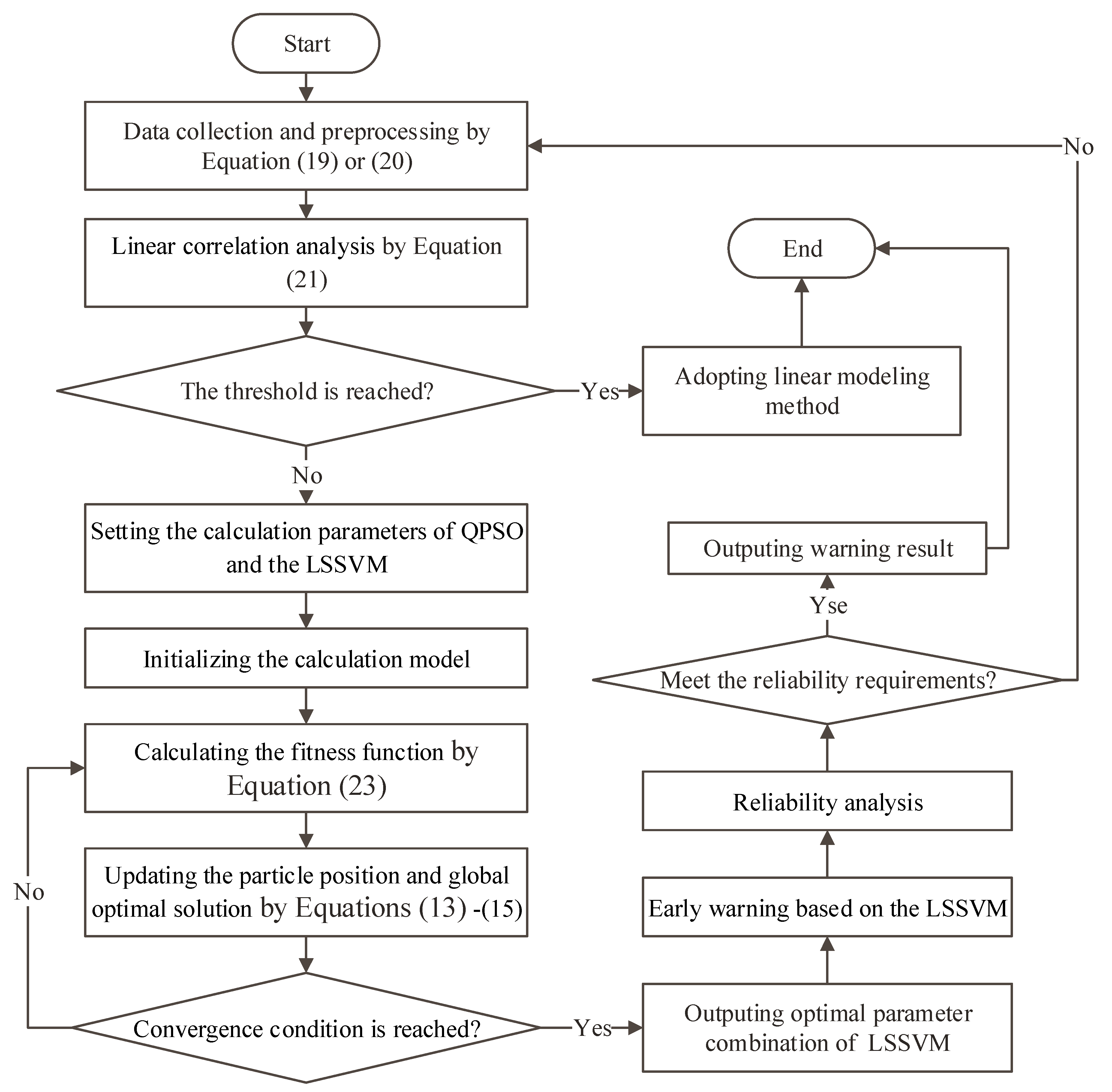
4.3. The Proposed Prediction Model

Step 1: Data collection and preprocessing

Data are obtained by on-site investigation and the consultation of construction logs and project management documents. Qualitative index data should be tested for reliability and validity.

To reduce the complexity of the modeling calculation of the LSSVM, the extreme value normalization method is adopted to standardize the data.

For benefit-based indicators [31]:

$$x_{ij}^{*}=\frac{x_{ij}-\min \left(x_j\right)}{\max \left(x_j\right)-\min \left(x_j\right)}.$$

(19)

For cost-based indicators [31]:

$$x_{ij}^{*}=\frac{\max \left(x_j\right)-x_{ij}}{\max \left(x_j\right)-\min \left(x_j\right)},$$

(20)

where $x_{ij}$ is the data of the $j$-th indicator of the $i$-th early warning object, $\min \left(x_j\right)$ represents the minimum value of the data of the $j$-th indicator, $\max \left(x_j\right)$ represents the maximum value of the data of the $j$-th indicator, and $x_{ij}^{*}$ is the normalized data.

Step 2: Linear correlation analysis

Choosing the linear or nonlinear modeling method is the first step of early risk warning. In this study, the Pearson correlation coefficient is selected to analyze the correlations between early warning indicators and early warning results. Its calculation formula is as follows [31]:

$$r=\frac{{{\displaystyle \sum }}_{i=1}^n\left(x_i-\overline{x}\right)\left(y_i-\overline{y}\right)}{\sqrt{{{\displaystyle \sum }}_{i=1}^n{\left(x_i-\overline{x}\right)}^2{\left(y_i-\overline{y}\right)}^2}},$$

(21)

where $x_i$ is the value of a certain early warning variable, $\overline{x}$ is the average value of a certain variable, $y_i$ is the risk early warning result, and $\overline{y}$ is the average value of the risk early warning result. If $r$ is greater than 0.7, there is only a certain linear correlation; if $r$ is less than 0.7, there is almost no linear correlation [32].

In this work, 70% is set as the threshold for selecting the modeling method. When more than 70% of the early warning indicators have an obvious linear relationship with the risk early warning results, the linear modeling method should be used for risk prediction. If most of the early warning indicators are linearly related to the results, it is suggested to adopt a linear modeling method or re-collect data.

Step 3: Searching for the optimal parameters of the LSSVM based on QPSO

(1)

Setting the calculation parameters of QPSO and the LSSVM.

Excluding the total number of particles $N$ and the maximum number of iterations $t_{max}$ in the population, the QPSO has only one parameter, namely the compression-expansion factor $\alpha \left(t\right)$. To simplify the algorithm to the greatest extent, the value strategy of α linear reduction is chosen for use [20]:

$$\alpha \left(t\right)=\frac{\left({\alpha }_1-{\alpha }_2\right)\left(t_{max}-t\right)}{t_{max}}+{\alpha }_2,$$

(22)

where ${\alpha }_1$ and ${\alpha }_2$ are the initial and termination values of $\alpha$, respectively, and ${\alpha }_1>{\alpha }_2$ is satisfied. It should be emphasized that the selection of calculation parameters of QPSO generally only affects the calculation efficiency of the algorithm and has little effect on the optimization results.

In the LSSVM, the regularization parameter and the width parameter of the kernel function are randomly given. However, the range of parameters should be as large as possible, so that the optimal parameter combination can be found.

(2)

Initializing the calculation model

The ratio of the training and test sets is set according to the research needs. The common ratios were 95%:5%, 90%:10%, 80%:20%, and 70%:30%.

The optimization model of QPSO is initialized according to Equations (13)–(15), and the nonlinear early warning model of the LSSVM is initialized according to Equations (16)–(18).

(3)

Calculating the fitness function

The regularization parameter and the width parameter are used as the solution dimensions in QPSO. The optimal kernel function parameters and penalty factor parameters in each iteration of QPSO are trained as the parameters of the LSSVM model, and the fitness values of all particles are calculated by the fitness function. The root-mean-square error ($RMSE$) is selected as the fitness function to evaluate QPSO [16,33]:

$$RMSE=\sqrt{\frac{1}{n}{{\displaystyle \sum }}_{i=1}^n{\left(y_i-{\widehat{y}}_i\right)}^2},$$

(23)

where $n$ is the number of samples in the test set, $y_i$ is the predicted value and ${\widehat{y}}_i$ is the true value.

(4)

Updating the particle position and global optimal solution according to the fitness function.

(5)

Judging whether the convergence condition is reached.

The convergence criterion of QPSO is usually that particles “gather” in a small range around a certain position. In this study, the following conditions must be met when converging [16]:

$$\max \left\{\left|u_i\left(t\right)-u_j\left(t\right)\right|\right\}<\epsilon ,$$

(24)

where $1\le i,j\le N$, and $i\ne j$. Moreover, $\epsilon$ is a small positive number, the value of which is considered 10⁻⁵ in this study.

If the convergence condition is not met, the optimization is continued. When the convergence condition is reached, the optimal parameter combination can be obtained.

Step 4: Construction risk early warning based on the LSSVM

The optimal parameter combination is introduced into Equations (16)–(18), and the LSSVM model is reconstructed for calculation so that the early warning result of the construction risk level can be obtained. It should be noted that, given the regularization parameter and the Gaussian kernel function width parameter, the LSSVM can conduct risk early warning. The purpose of Step 3 is to find the optimal calculation parameters of the LSSVM.

Step 5: Reliability analysis of the early warning results

To verify the reliability of the early warning results, the Bland–Atman analysis method is used to analyze the early warning values and the measured values. The Bland–Atman analysis is realized with the assistance of SPSS 17.0 software.

If the early warning result based on the proposed method is consistent with the true value within the 95% confidence interval, it indicates that the early warning result has good reliability and the early warning is over. Otherwise, Steps 3 and 4 are repeated.

Summarizing the above analysis, the flowchart of the proposed model was shown in Figure 1.

It should be emphasized that the proposed model was a data-driven model. Different cases mean different engineering data and different trained models. However, the proposed model, rather than trained models, is able to be applied to any type of case study.

5. Case Analysis

5.1. Project Overview and Data Acquisition

The total length of Chengdu Metro Line 11 in China is 22.0 km, and it has 17 new subway stations. The engineering profiles of the 17 stations are presented in

Table 4. The overview of the 17 stations.

Station	Maximum Excavation Depth	Regional Characteristics	Contractor	Adverse Conditions
Huilong Boulevard Station	21.26 m	Urban region under construction	CCTEB	Abandoned pipe gallery, high slope
Science Park Station	18.65 m	Urban region under construction	CCTEB	Abandoned pipe gallery
Science Park East Station	19.75 m	Urban region under construction	CCTEB	Fish pond, gas pipeline, high-voltage electric tower
Science Park South Station	25.18 m	Urban region under construction	CCTEB	Rivers, high gas
Wan’an Station	21.45 m	Urban region under construction	CCTEB	Multiple ponds, high gas
Lushan Boulevard Station	28.84 m	Established urban region	CCTEB	Under a bridge, high gas.
Shenyang Road Station	19.45 m	Established urban region	CSCRIE	Many ponds and rivers, high-voltage lines, high gas.
Dakoujing Station	18.46 m	Established urban region	CSCRIE	Many projects under construction, high gas
Miaoyan Station	26.47 m	Established urban region	CCTEB	High gas
Tianfu CBD North Station	28.80 m	Urban region under construction	CSCRIE	High voltage tower
Tianfu CBD East Station	22.50 m	Urban region under construction	CSCRIE	Large bridge
Guobin Boulevard station	24.37 m	Urban region under construction	CSCRIE	Utility tunnel, underpass tunnel, viaduct
Lujiao Village Station	19.57 m	Urban region under construction	CSCRIE	Ponds, chemical tanks, high-voltage wire towers, projects under construction
Diaoyuzui East Station	18.50 m	Suburban region	CCTEB	Ponds
Diaoyuzui Station	19.85 m	Suburban region	CCTEB	Flood channel, high slope, landscape bridge
Huilong Road Station	20.75 m	Suburban region	CCTEB	Low terrain, rivers, existing subway line
Huilonglu West station	22.46 m	Suburban region	CCTEB	Ponds, slopes, rivers

.

Due to spatial constraints, Table 4 only reports the four most important types of station information, namely the maximum excavation depth, regional characteristics, construction units, and unfavorable conditions.

The maximum excavation depth is the most important factor affecting the construction difficulty of subway station engineering. The greater the excavation depth, the higher the professional skills of the construction workers, the higher the management ability of the project managers, the higher the quality and maintenance level of the construction machinery, and the higher the quality of construction materials. In addition, the deeper the subway station project, the more easily it will experience adverse effects from the surrounding environment.

Regional characteristics reflect the availability of construction machinery and construction materials. In urban areas, due to traffic control, it is difficult to promptly obtain construction materials. In the suburbs and newly-built development zones, construction materials can easily be promptly obtained. In addition, subway station projects with different regional characteristics suffer from different unfavorable environmental factors.

Relevant information about the construction unit directly reflects the risk management level of the project management team. The construction units of this project are the China Construction Third Engineering Bureau Group Co., Ltd., Wuhan, China (hereinafter referred to as CCTEB) and the China State Construction Railway Investment & Engineering Group Co., Ltd., Wuhan, China (hereinafter referred to as CSCRIE). CCTEB has rich experience in subway station engineering construction, while CSCRIE lacks relevant construction experience.

Unfavorable conditions mainly include unfavorable geological conditions, unfavorable geomorphic conditions, and extreme weather conditions, all of which are important causes of construction safety accidents. Excluding Wan’an Station, Dakoujing Station, Guobin Avenue Station, Fishing Mouth East Station, Fishing Mouth Station, and Huilong Road West Station, the other stations are characterized by complicated pipelines, which affect the construction.

According to the index data acquisition methods described in Section 3.3, 294 groups of data were collected. After eliminating invalid data, 261 groups of valid data were retained, as shown in

Table 5. Partial case data.

No.	1	2	3	4	5	$\cdots$	257	258	259	260	261
Risk Level	II	III	I	II	II		IV	II	II	I	III
$R_{11}$	1.47	3.45	0.12	2.62	0.88	$\cdots$	4.01	1.34	5.76	4.90	2.62
$R_{12}$	5.89	5.9	8.04	2.52	4.11	$\cdots$	2.77	6.08	7.93	7.26	2.44
$R_{13}$	5	4	0	1	5	$\cdots$	13	9	1	7	3
$R_{14}$	5.46	2.47	3.19	9.94	4.61	$\cdots$	10.07	6.65	2.96	5.41	9.86
$R_{15}$	10.90	21.81	13.73	18.50	6.82	$\cdots$	10.92	7.46	20.35	10.14	5.37
$R_{21}$	3.18	3.76	4.50	3.69	2.67	$\cdots$	1.71	4.80	4.49	4.10	3.36
$R_{22}$	0.21	1.62	0.06	0.87	1.64	$\cdots$	1.07	1.86	0.29	1.29	2.00
$R_{23}$	0.29	5.54	6.54	2.97	3.74	$\cdots$	5.12	3.26	5.33	5.98	5.65
$R_{31}$	98.77	99.15	99.55	99.68	99.64	$\cdots$	98.77	99.66	98.92	98.44	98.94
$R_{32}$	99.58	98.5	98.18	99.51	98.67	$\cdots$	99.97	99.21	98.98	99.71	98.70
$R_{33}$	99.67	97.10	97.98	97.77	95.19	$\cdots$	95.91	98.23	95.99	97.10	96.69
$R_{34}$	2.45	3.58	2.93	2.77	0.49	$\cdots$	1.29	1.26	3.24	0.84	2.10
$R_{41}$	28.20	21.03	24.14	7.90	21.41	$\cdots$	33.33	6.98	13.01	30.57	6.90
$R_{42}$	167	0	0	5	55	$\cdots$	0	0	15	120	10
$R_{43}$	34.5	35	37.5	44	33.5	$\cdots$	38	47.5	35	46	49
$R_{44}$	65	71	74.5	13	36	$\cdots$	52	51.5	57	85	73.5
$R_{45}$	30	32.5	36	10	22.5	$\cdots$	27	24.5	28	29.5	19
$R_{51}$	10	14.5	19	13.5	13	$\cdots$	18	10.5	20	12.5	15.5
$R_{52}$	11	19.5	180	16	19.5	$\cdots$	17	17.5	18	13	16
$R_{53}$	13.58	12.57	13.98	14.69	18.69	$\cdots$	15.19	15.89	11.99	13.43	18.51
$R_{54}$	24	24.5	27	26.5	17	$\cdots$	16.5	26	14.5	11	12.5

. Due to spatial limitations, only partial data are provided in Table 5. It should be emphasized that 261 sets of data represent a small data set for simulation but a large data set for a case study.

Table 1 presents the information of the experts who participated in determining the qualitative indicators. The Cronbach’s alpha values of all qualitative indicators were found to be greater than 0.7, which proves the reliability of the questionnaire survey results [34].

5.2. Data Preprocessing and Correlation Analysis

According to the type of indicator, the normalized early warning data could be obtained by introducing the data in Table 5 into Equation (19) or (20). The normalized early warning data were then introduced into Equation (21) to obtain the correlation analysis results of each index (input variable) and the early warning level (output variable), as shown in

Table 6. The correlations between the secondary indexes and risk early warning results.

Secondary index	$R_{11}$	$R_{12}$	$R_{13}$	$R_{14}$	$R_{15}$	$R_{21}$	$R_{22}$
Pearson correlation coefficient	−0.4871	−0.7124	0.5767	−0.7521	0.1574	0.8017	−0.2578
Secondary index	$R_{23}$	$R_{31}$	$R_{32}$	$R_{33}$	$R_{34}$	$R_{41}$	$R_{42}$
Pearson correlation coefficient	−0.7533	0.4297	0.8746	0.3325	−0.1247	0.7197	−0.5427
Secondary index	$R_{43}$	$R_{44}$	$R_{45}$	$R_{51}$	$R_{52}$	$R_{53}$	$R_{54}$
Pearson correlation coefficient	0.3475	0.2458	−0.3462	0.746	0.3024	−0.7003	−0.2467

.

Among the 21 secondary indicators, the absolute values of the Pearson correlation coefficients of only eight indicators were greater than 0.7. Only 38.09% of the secondary indicators had an obvious linear relationship with the early warning results of construction risks. Therefore, the nonlinear modeling method was chosen for the case study.

5.3. Early Warning of Construction Safety Risks

(1)

Set the parameters of algorithms

The $t_{max}$ of QPSO was set to 1000, and the $N$ was set to 20 [18,20]. Moreover, the compression-expansion factors were set to ${\alpha }_1=0.8$ and ${\alpha }_2=0.4$. According to Equation (22),

$${\alpha }_t=0.4\left(1-\frac{t}{t_{max}}\right)+0.4.$$

(25)

The range of the $\mathrm{C}$ is [0.01, 10], and the range of the width parameter $\sigma$ of the kernel function is [10, 1000] [13]. The initial regularization parameter of the LSSVM is 2, and the initial width parameter is 30.

(2)

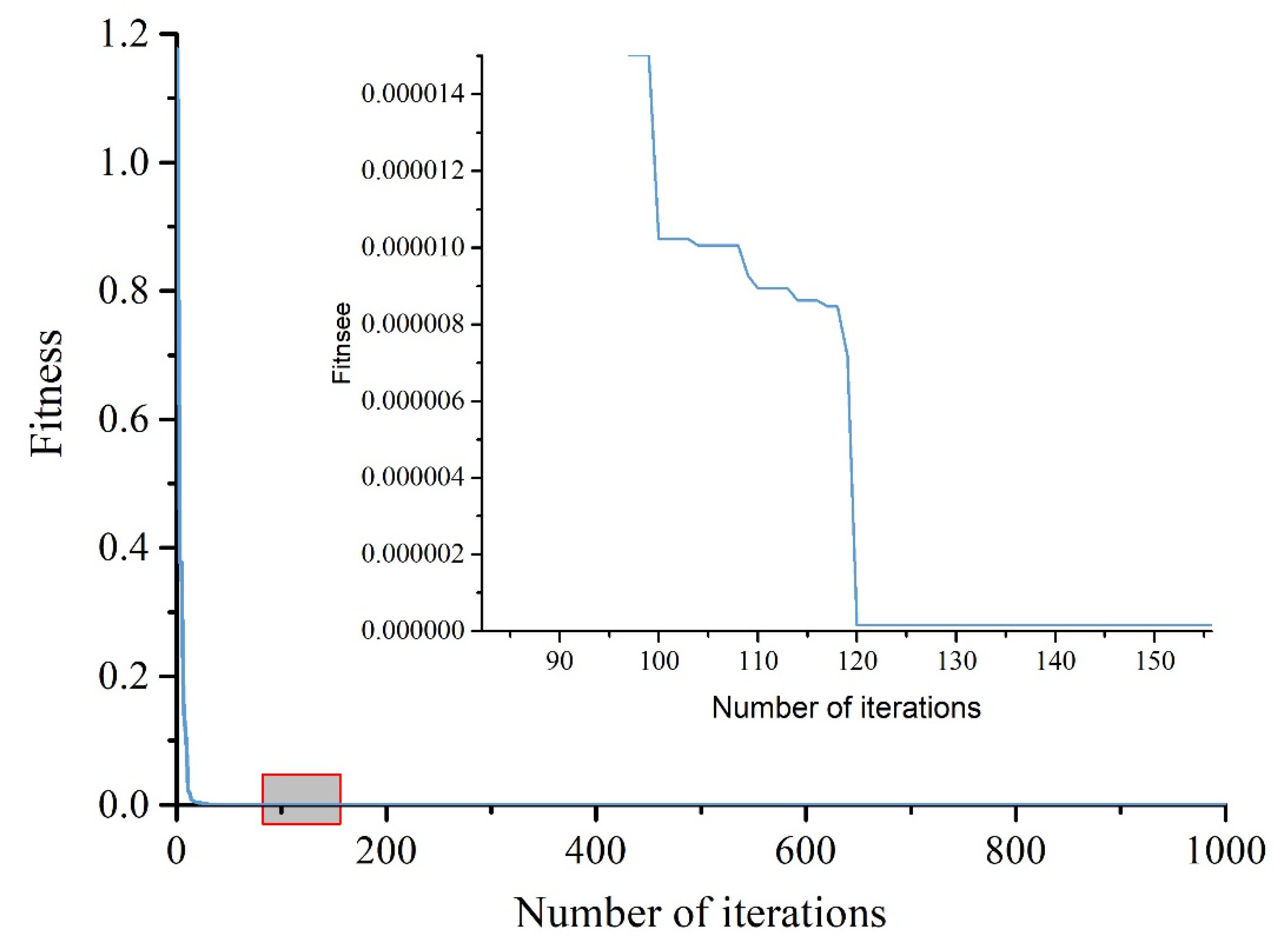
Find the optimal parameter combination of the LSSVM based on QPSO

The normalized data and preset QPSO parameters were introduced into Equations (13)–(15) to initialize the optimization model of QPSO. Then, the normalized data and preset LSSVM calculation parameters were introduced into Equations (16)–(18) to initialize the LSSVM-based nonlinear early warning model. All the calculation programs were realized with the assistance of MATLAB 2016 software.

The initial fitness function was calculated, and the particle position and global optimal solution were updated according to the fitness function. The fitness function of QPSO is shown in Figure 2.

The QPSO found the optimal calculation parameters of LSSVM around the 120th generation. The best regularization parameter was 1.742, and the best width parameter was 14.167. The iterative steps of QPSO around the 120th generation were tracked in detail, as exhibited in

Table 7. Detailed QPSO update process.

Iterations	Fitness of the k − 1 Iteration	Fitness of the k Iteration	Accuracy	Continue?
118	0.0000084643	0.0000084643	0 < 0.0000001	Yes
119	0.0000084643	0.0000071867	0.0000012776 > 0.0000001	Yes
120	0.0000071867	0.0000001597	0.0000070270 > 0.0000001	Yes
1000	0.0000001597	0.0000001597	0 < 0.0000001	No

.

Table 7 reveals that QPSO found the optimal calculation parameters of the LSSVM in the 120th generation. To examine the stability of QPSO calculations, the proposed model was recalculated 100 times. The QPSO found the best calculation parameters of LSSVM after 134.71 optimization times on average.

(3)

Construction of the early warning model based on the LSSVM

Among all data sets, 234 were randomly selected as training sets, and the remaining 27 were used as test sets. Thus, the ratio of the training sets to the test sets was 89.66%:10.34%. This ratio is discussed in detail in Section 6.3.

All data and calculation parameters were introduced back into Equations (16)–(18), and the nonlinear early warning model based on the LSSVM was calculated. The calculation results of the test set are reported in

Table 8. The prediction results of the test set.

Test Set	Actual Risk	The Predicted Results	Test Set	Actual Risk	The Predicted Results
1	II	II (2.003)	141	III	III (2.985)
11	II	II (1.986)	151	I	II (1.975)
21	III	III (3.014)	161	II	II (2.037)
31	I	I (0.997)	171	III	III (3.004)
41	IV	IV (4.006)	181	IV	IV (3.995)
51	II	II (2.013)	191	II	II (2.007)
61	I	I (1.012)	201	III	III (3.014)
71	II	II (2.004)	211	I	I (1.005)
81	III	III (2.987)	221	II	II (2.003)
91	I	I (1.001)	231	III	III (3.014)
101	III	III (3.027)	241	I	I (1.027)
111	II	II (2.001)	251	II	II (2.002)
121	I	I (1.000)	261	III	III (2.999)
131	II	II (1.998)	-	-	-

. Sample data with the wrong prediction in Table 8 are bolded.

Among the 27 test set samples, only the 151 test set had the wrong prediction. The error rate of the proposed model was 3.7%. It should be emphasized that this is the result of a prediction calculation.

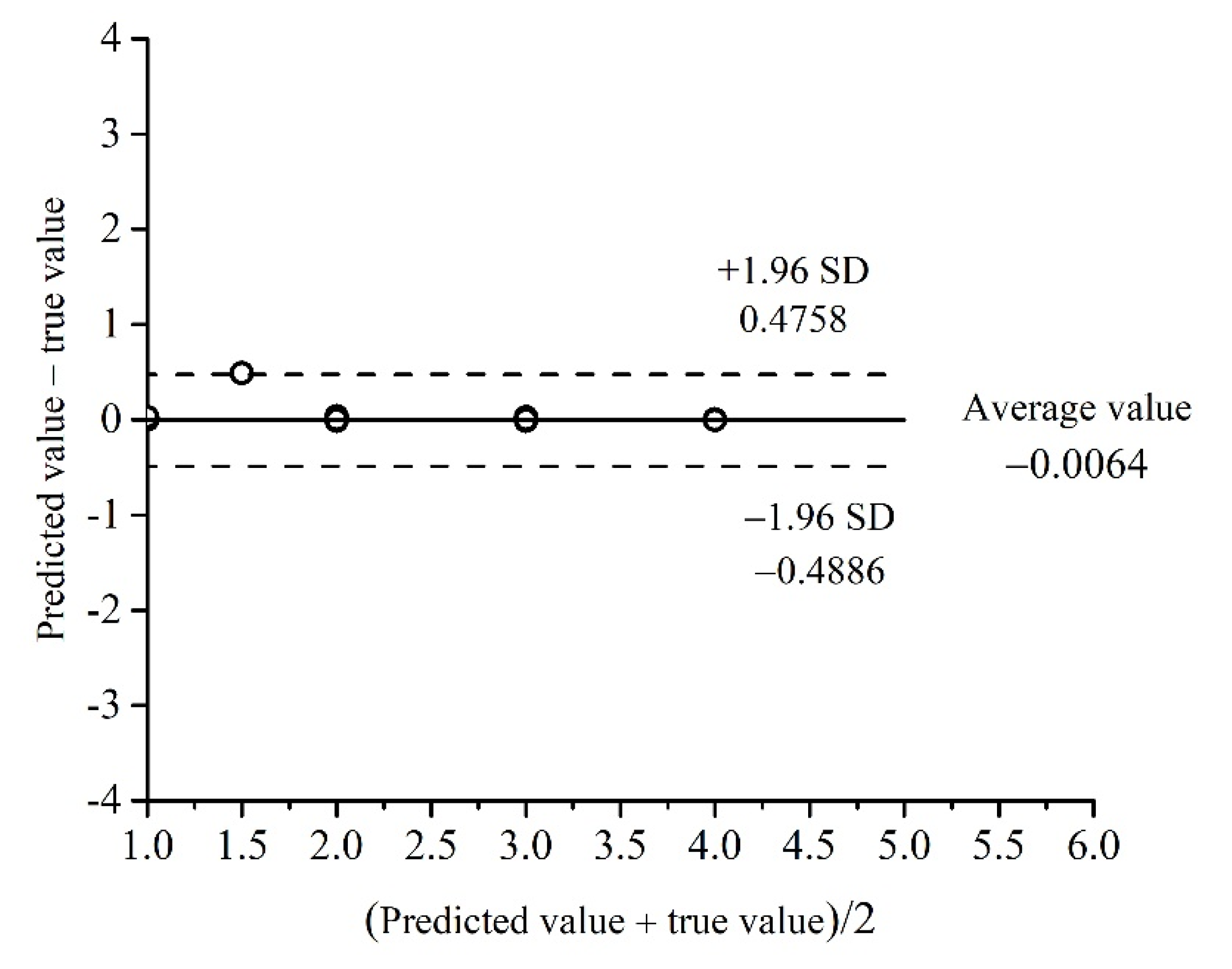
5.4. Reliability Analysis of Early Warning Results

To testify the reliability of the predicted results in Section 5.3, the Bland–Altman analysis was used to analyze the predicted values and the measured values. The Bland–Altman analysis method was first put forward by British scholars Bland and Altman in 1983. Its basic principle is to analyze the differences between the results calculated by two different methods within a 95% confidence interval (consistency limit). This method has become an authoritative statistical method to judge the consistency of the results calculated by two data calculation methods. In this research, the calculation results based on QPSO-LSSVM and the real construction risks were compared. If the calculation results based on QPSO-LSSVM were consistent with the real construction risks within a 95% confidence interval, it showed that the risk warning results based on QPSO-LSSVM had good reliability. In the empirical study, the Bland–Altman diagram is shown in Figure 3.

In Figure 3, the vertical axis of the diagram was the difference between the measured value and the predicted value, and the horizontal axis was the average of the measured value and the predicted value of the model. From Figure 3, 26 groups of values were within $\left(-1.96\mathrm{SD},+1.96\mathrm{SD}\right)$, and only one group was absent. According to the basic principle of the Bland–Altman analysis method, it could be known that the calculated results in Section 5.3 and the measured values met 95% of the predicted points within the consistency range. Therefore, the early warning results of construction risks in Section 5.3 had high reliability.

6. Discussion

6.1. Computational Performance of Different Optimization Algorithms

Although many research results have proved the excellent computing performance of QPSO in many optimization problems, there has been little research on the optimization performance of QPSO in the LSSVM model. The computational performance of different meta-heuristic optimization algorithms in different studies is likely to be significantly different [35]. Classical and latest meta-heuristic optimization algorithms (GA [11], PSO [36], GSA [14], WOA [14]) were selected to find the best calculation parameters in Section 5. The calculation parameters and principles of each algorithm refer to the corresponding references. In addition, TE [14], a classical LSSVM parameter determination method, was selected to perform calculations. The results of 100 calculations of different optimization algorithms are shown in

Table 9. Calculation results of different optimization algorithms.

Optimization Algorithm	Average Number of Misjudgments	Average Prediction Error	Average Calculation Time	Average Iteration Times at Convergence
TE	4.14	24.35%	-	-
GA	1.01	5.94%	1574.24	574.14
PSO	1.27	7.47%	654.04	377.08
GSA	1.05	6.18%	317.17	229.07
WOA	1.24	7.29%	357.81	197.43
QPSO	0.75	4.41%	203.38	134.71

.

It could be seen from Table 9 that, compared with other meta-heuristic optimization algorithms, the calculation error of QPSO was the smallest, and the best calculation parameters of LSSVM could be found fastest with the QPSO.

By researchers’ manual trial and error, the TE method could find the appropriate LSSVM calculation parameters, which was understood as finding the LSSVM calculation parameters without using an optimization algorithm. The calculation error of the TE was the largest. This result emphasized the necessity of introducing an optimization algorithm into LSSVM research.

Generally, the algorithm performance is judged by the following three conditions. The best case indicates the fastest optimization speed of the algorithm. Average means the average of the algorithm. In the worst case, it means that the algorithm cannot find the optimal solution. The best case is accidental, so it has no comparative value, and the average case has been discussed in this section. Therefore, this section will continue to discuss the worst case.

The range of the $\mathrm{C}$ was reset to [100, 10,000], and the range of the width parameter $\sigma$ was reset to [0.001, 10]. The optimal combination of parameters was not in this interval, so the three optimization algorithms could not find the optimal solution within the maximum iteration steps. After calculation, it was found that QPSO completed the calculation fastest, so the complexity of QPSO was the smallest among all algorithms.

6.2. Computational Performance of Different Prediction Methods

To compare the computational performance of the proposed model, the BPNN and Extreme Learning Machine (ELM) [37] were selected for comparative analysis. The two data prediction methods also use QPSO to get the optimal calculation parameters, and the calculation results of 100 calculations were shown in

Table 10. Calculation results of different early warning models.

Early Warning Model	QPSO-BP	QPSO-ELM	QPSO-LSSVM
Average number of misjudgments	3.28	1.74	0.75
Average prediction error	19.29%	10.24%	4.41%
Average calculation time	687.52	374.24	203.38
Average iteration times at convergence	439.34	233.01	134.71

.

It could be seen from Table 10 that the early warning error rate of QPSO-LSSVM was only 4.41%, and the early warning accuracy was significantly higher than that of QPSO-BP and QPSO-ELM. The prediction model constructed by BPNN had the largest misjudgment rate, which was 4.37 times that based on the LSSVM model. Under the same optimization algorithm, the average calculation time of LSSVM was the shortest, and the optimal solution could be found the fastest. It was considered that this method had the advantages of being a simple model and having a fast calculation speed.

According to the calculation principles of the three algorithms, the LSSVM determined the segmentation hyperplane only with fewer support vectors, while BPNN or ELM followed the law of large numbers in nonlinear modeling [38]. When the training data samples of BPNN or ELM were more, their prediction results were closer to the truth. The number of sample sets of BPNN or ELM was often required to be more than ten times that of input variables. Therefore, under the condition of sufficient historical data and large research samples, the BPNN or ELM method had more advantages than LSSVM in nonlinear modeling ability and computational performance. However, when the historical data was insufficient or the research samples were small, the nonlinear modeling ability and computational performance of LSSVM were significantly better than those of the BPNN or ELM methods.

6.3. The Influence of the Different Ratios of Training Sets and Test Sets

In the research of machine learning, the ratio of the training set to the test set might affect the calculation results. These common proportions mentioned in Section 4.3 were selected to warn the construction safety risks of the case objects. The results of 100 calculations with different ratios of training sets and test sets are shown in

Table 11. Calculation results of the different ratios.

Ratio of Training Set and Test Set	Average Number of Misjudgments	Average Prediction Error	Bland–Altman Analysis
247:14 94.64%:5.36%	0.23	1.64%	Pass
234:17 89.66%:10.34%	0.75	4.41%	Pass
208:53 79.69%:20.31%	2.26	4.26%	Pass
182:79 69.73%:30.27%	7.54	9.54%	Fail

below.

It could be seen that with the decreasing number of samples in the training set, the prediction error gradually increased, in which the average number of misjudgments increased from 0.23 to 7.54, and the average prediction error increased from 1.64% to 9.54%. While the ratio of the sample set to test set was 69.73%:30.27%, the average prediction error was close to 10%, and it failed to pass the Bland–Altman analysis. Therefore, it was reasonable to set the ratio of the training set to testing set to 89.66%:10.34% in Section 5. In addition, the sample set ratio should not be lower than 80% when using this proposed model.

7. Conclusions

In this paper, an early warning model of subway station construction safety risk based on QPSO and LSSVM was developed, and a case study of Chengdu Metro Line 11 was carried out. Based on the theory of accident cause and the characteristics of subway station engineering, an early warning index system of subway station engineering construction safety risk was constructed. Among the 21 secondary indicators in this index system, only 8 indicators had an obvious linear relationship with the early warning results of construction risks. This showed that the nonlinear modeling method should be used in the early warning research on subway station construction safety risks. The LSSVM with strong nonlinear analysis abilities and QPSO with strong global retrieval ability were used to construct the early warning model. In the case analysis, QPSO found the optimal calculation parameters of LSSVM in the 120th generation, and the error rate of the model proposed was only 3.7%. Bland–Altman analysis also proved that the early warning result of case analysis is very reliable. Compared with other meta-heuristic optimization algorithms such as GA, PSO, GSA, and WOA, QPSO had the smallest calculation error and could find the best calculation parameters of LSSVM as quickly as possible. Compared with BPNN and ELM, the proposed model had a better computational performance. The influence of the ratio setting of the training set and testing set on the early warning results was also discussed.

Although the engineering practice data collected in this study met the needs of this study, there was still a gap in the ideal number of samples. In the future, more relevant engineering practice materials (such as subway station projects in different countries or different regions) could be obtained to further verify the scientificity, effectiveness and advancement of this research method.

References

1. Haddad, E.A.; Hewings, G.J.D.; Porsse, A.A.; Van Leeuwen, E.S.; Vieira, R.S. The underground economy: Tracking the higher-order economic impacts of the Sao Paulo Subway System. Transp. Res. Part A Policy Pract. 2015, 73, 18–30. [Google Scholar] [CrossRef]
2. Zhou, Z.; Irizarry, J.; Li, Q. Using network theory to explore the complexity of subway construction accident network (SCAN) for promoting safety management. Saf. Sci. 2014, 64, 127–136. [Google Scholar] [CrossRef]
3. Merz, B.; Kuhlicke, C.; Kunz, M.; Pittore, M.; Babeyko, A.; Bresch, D.N.; Domeisen, D.I.V.; Feser, F.; Koszalka, I.; Kreibich, H.; et al. Impact Forecasting to Support Emergency Management of Natural Hazards. Rev. Geophys. 2020, 58, e2020RG000704. [Google Scholar] [CrossRef]
4. Liu, L.; Wu, H.; Wang, J.; Yang, T. Research on the evaluation of the resilience of subway station projects to waterlogging disasters based on the projection pursuit model. Math. Biosci. Eng. 2020, 17, 7302–7331. [Google Scholar] [CrossRef]
5. Sjekavica Klepop, M.; Radujkovic, M. Early Warning System in Managing Water Infrastructre Projects. J. Civ. Eng. Manag. 2019, 25, 531–550. [Google Scholar] [CrossRef] [Green Version]
6. Qiu, H.; Yu, X.; Dong, J. Risk Factor Prediction Model of Oil and Gas Construction Project Based on Combination Mathematical Model. Ekoloji 2019, 28, 4033–4043. [Google Scholar]
7. Senthil, J.; Muthukannan, M. Predication of construction risk management in modified historical simulation statistical methods. Ecol. Inform. 2021, 66, 101439. [Google Scholar] [CrossRef]
8. Yadav, A.K.; Chandel, S.S. Identification of relevant input variables for prediction of 1-minute time step photovoltaic module power using Artificial Neural Network and Multiple Linear Regression Models. Renew. Sustain. Energy Rev. 2017, 77, 955–969. [Google Scholar] [CrossRef]
9. Shen, T.; Nagai, Y.; Gao, C. Design of building construction safety prediction model based on optimized BP neural network algorithm. Soft Comput. 2020, 24, 7839–7850. [Google Scholar] [CrossRef]
10. Yaseen, Z.M.; Ali, Z.H.; Salih, S.Q.; Al-Ansari, N. Prediction of Risk Delay in Construction Projects Using a Hybrid Artificial Intelligence Model. Sustainability 2020, 12, 1514. [Google Scholar] [CrossRef] [Green Version]
11. Liu, P.; Xie, M.; Bian, J.; Li, H.; Song, L. A Hybrid PSO-SVM Model Based on Safety Risk Prediction for the Design Process in Metro Station Construction. Int. J. Environ. Res. Public Health 2020, 17, 1714. [Google Scholar] [CrossRef] [PubMed] [Green Version]
12. Yusuf, F.; Olayiwola, T.; Afagwu, C. Application of Artificial Intelligence-based predictive methods in Ionic liquid studies: A review. Fluid Phase Equilibria 2021, 531, 112898. [Google Scholar] [CrossRef]
13. Huang, J.; Liang, Y.; Bian, H.; Wang, X. Using Cluster Analysis and Least Square Support Vector Machine to Predicting Power Demand for the Next-Day. IEEE Access 2019, 7, 82681–82692. [Google Scholar] [CrossRef]
14. Zeng, F.; Nait Amar, M.; Mohammed, A.S.; Motahari, M.R.; Hasanipanah, M. Improving the performance of LSSVM model in predicting the safety factor for circular failure slope through optimization algorithms. Eng. Comput. 2021. [Google Scholar] [CrossRef]
15. Cui, G.; Xiong, S.; Zhou, C.; Liu, Z. Research on HC-LSSVM Model for Soft Soil Settlement Prediction Based on Homotopy Continuation Method. Appl. Sci. 2021, 11, 10666. [Google Scholar] [CrossRef]
16. Zhu, X.; Ma, S.-q.; Xu, Q.; Liu, W.-d. A WD-GA-LSSVM model for rainfall-triggered landslide displacement prediction. J. Mt. Sci. 2018, 15, 156–166. [Google Scholar] [CrossRef]
17. Noori, A.M.; Mikaeil, R.; Mokhtarian, M.; Haghshenas, S.S.; Foroughi, M. Feasibility of Intelligent Models for Prediction of Utilization Factor of TBM. Geotech. Geol. Eng. 2020, 38, 3125–3143. [Google Scholar] [CrossRef]
18. Sun, J.; Wu, X.; Palade, V.; Fang, W.; Lai, C.-H.; Xu, W. Convergence analysis and improvements of quantum-behaved particle swarm optimization. Inf. Sci. 2012, 193, 81–103. [Google Scholar] [CrossRef]
19. Alajmi, M.S.; Almeshal, A.M. Prediction and Optimization of Surface Roughness in a Turning Process Using the ANFIS-QPSO Method. Materials 2020, 13, 2986. [Google Scholar] [CrossRef]
20. Yang, L.; Fu, Y.; Wang, Z.; Zhen, X.; Yang, Z.; Fan, X. An Optimized Level Set Method Based on QPSO and Fuzzy Clustering. IEICE Trans. Inf. Syst. 2019, E102D, 1065–1072. [Google Scholar] [CrossRef] [Green Version]
21. Sun, J.; Fang, W.; Wang, D.; Xu, W. Solving the economic dispatch problem with a modified quantum-behaved particle swarm optimization method. Energy Convers. Manag. 2009, 50, 2967–2975. [Google Scholar] [CrossRef]
22. Singh, J.; Verma, A.K.; Banka, H.; Singh, T.N.; Maheshwar, S. A study of soft computing models for prediction of longitudinal wave velocity. Arab. J. Geosci. 2016, 9, 224. [Google Scholar] [CrossRef]
23. Hyungju, K.; Stein, H.; Bouwer, U.I. Assessment of accident theories for major accidents focusing on the MV SEWOL disaster: Similarities, differences, and discussion for a combined approach. Saf. Sci. 2016, 82, 410–420. [Google Scholar] [CrossRef]
24. Li, W.; Zhang, L.; Liang, W. An Accident Causation Analysis and Taxonomy (ACAT) model of complex industrial system from both system safety and control theory perspectives. Saf. Sci. 2017, 92, 94–103. [Google Scholar] [CrossRef]
25. Zhang, S.; Sunindijo, R.Y.; Loosemore, M.; Wang, S.; Gu, Y.; Li, H. Identifying critical factors influencing the safety of Chinese subway construction projects. Eng. Constr. Archit. Manag. 2021, 28, 1863–1886. [Google Scholar] [CrossRef]
26. Yue, Y.; Xiahou, X.; Li, Q. Critical Factors of Promoting Design for Safety in China’s Subway Engineering Industry. Int. J. Environ. Res. Public Health 2020, 17, 3373. [Google Scholar] [CrossRef]
27. Wu, H.; Wang, J. Assessment of Waterlogging Risk in the Deep Foundation Pit Projects Based on Projection Pursuit Model. Adv. Civ. Eng. 2020, 2020, 2569531. [Google Scholar] [CrossRef]
28. Liu, X.; Chen, H. Integrated assessment of ecological risk for multi-hazards in Guangdong province in southeastern China. Geomat. Nat. Hazards Risk 2019, 10, 2069–2093. [Google Scholar] [CrossRef]
29. Xia, C.; Nie, G.; Li, H.; Fan, X.; Yang, R. Study on the seismic lethal level of buildings and seismic disaster risk in Guangzhou, China. Geomat. Nat. Hazards Risk 2022, 13, 800–829. [Google Scholar] [CrossRef]
30. Zhou, M.; Kuang, Y.; Ruan, Z.; Xie, M. Geospatial modeling of the tropical cyclone risk in the Guangdong Province, China. Geomat. Nat. Hazards Risk 2021, 12, 2931–2955. [Google Scholar] [CrossRef]
31. Wu, H.; Wang, J. A Method for Prediction of Waterlogging Economic Losses in a Subway Station Project. Mathematics 2021, 9, 1421. [Google Scholar] [CrossRef]
32. Zhang, H.; Yu, T. Prediction of subgrade elastic moduli in different seasons based on BP neural network technology. Road Mater. Pavement Des. 2018, 19, 271–288. [Google Scholar] [CrossRef]
33. Ahmadi, H.; Ahmadi, H.; Baghban, A. Modeling vaporization enthalpy of pure hydrocarbons and petroleum fractions using LSSVM approach. Energy Sources Part A Recovery Util. Environ. Eff. 2020, 42, 569–576. [Google Scholar] [CrossRef]
34. Bujang, M.A.; Omar, E.D.; Baharum, N.A. A Review on Sample Size Determination for Cronbach’s Alpha Test: A Simple Guide for Researchers. Malays. J. Med. Sci. 2018, 25, 85–99. [Google Scholar] [CrossRef]
35. Salemi, A.; Mikaeil, R.; Haghshenas, S.S. Integration of Finite Difference Method and Genetic Algorithm to Seismic analysis of Circular Shallow Tunnels (Case Study: Tabriz Urban Railway Tunnels). KSCE J. Civ. Eng. 2018, 22, 1978–1990. [Google Scholar] [CrossRef]
36. Mikaeil, R.; Haghshenas, S.S.; Sedaghati, Z. Geotechnical risk evaluation of tunneling projects using optimization techniques (case study: The second part of Emamzade Hashem tunnel). Nat. Hazards 2019, 97, 1099–1113. [Google Scholar] [CrossRef]
37. Huang, G.; Huang, G.-B.; Song, S.; You, K. Trends in extreme learning machines: A review. Neural Netw. 2015, 61, 32–48. [Google Scholar] [CrossRef]
38. Verma, A.K.; Sirvaiya, A. Comparative analysis of intelligent models for prediction of Langmuir constants for CO2 adsorption of Gondwana coals in India. Geomech. Geophys. Geo-Energy Geo-Resour. 2016, 2, 97–109. [Google Scholar] [CrossRef] [Green Version]
Figure 1. The flowchart of the proposed model.
Applsci 12 05712 g001
Figure 2. The fitness function of QPSO.
Applsci 12 05712 g002
Figure 3. Bland–Altman analysis.
Applsci 12 05712 g003