Improved Cutting Force Modelling in Micro-Milling Aluminum Alloy LF 21 Considering Tool Wear

Abstract

Aluminum alloy LF 21 has a strong ability to reflect electromagnetic waves. LF 21 waveguide slit array structure is widely used in waveguide radar antenna. The stiffness of the slit array structure is relatively weak. So, the structure is prone to deformation under the cutting force in the conventional milling process. Micro-milling technology can realize high-precision machining of mesoscale parts/structures and is a potential effective machining technology for the waveguide slit array structure. However, the diameter of the micro-milling cutter is small, and the feed per tooth is comparable to the arc radius of the cutting edge, so the micro-milling cutter is prone to wear. In addition, the effects of elastic recovery of material, the minimum cutting thickness and friction of cutting dead zone on micro-milling force cannot be ignored. A simulation model of micro-milling aluminum alloy LF 21 processes based on DEFORM 3D is built by combining the theory of cutting and the technology of process simulation. Prediction of tool wear is achieved. The quantitative relationship between the arc radius of the cutting edge and tool wear is clarified for the first time. The authors built an improved cutting force model in micro-milling LF 21 considering tool wear and cutter runout with the minimum cutting thickness as the boundary. The validity of the built micro-milling force model is verified by experiments.

1. Introduction

Aluminum alloy LF 21 has a strong ability to reflect electromagnetic waves. LF 21 waveguide slit array structure is widely used in waveguide radar antenna. The stiffness of the slit array structure is relatively weak. So, the structure is prone to deformation under the cutting force in conventional milling processes. Micro-milling technology can realize high-precision machining of mesoscale parts/structures, which is a potential effective machining technology for waveguide thin slot array structures. However, the small diameter and the low stiffness of the micro-milling cutter, the feed per tooth similarly sized the arc radius of the cutting edge, causes the micro-milling cutter to wear easily. The factors affecting the micro-milling force, such as tool wear, elastic recovery of material, the minimum cutting thickness and friction of metal cutting dead zone, etc., cannot be ignored. Yet, so far, few studies have reported to explore micro-milling aluminum alloy LF 21.

Simulation is an effective method to study the tool wear in micro-milling. Thepsonthi and Özel conducted in-depth research on the tool wear of micro-milling titanium alloyTi6Al-4V and simulated full-immersion and semi-immersion straight-inverse milling processes based on DEFORM 3D [1] and DEFORM 2D [2], respectively. They revealed that 3D simulation contributed to exploring the distribution of tool wear, tool wear led to the increase in negative rake angle and the tool wear in down-milling was slower than that in up-milling. Lu et al. utilized DEFORM 3D to simulate micro-milling nickel-based superalloy Inconel 718 and realized the prediction of tool flank wear [3]. Meng Jie et al. [4] introduced the coefficient of the size effect into the Usui wear model, calibrated the coefficient through experiments, and then established a 2D simulation model of the micro-milling AISI4340 alloy steel process based on Abaqus/CAE, achieving the prediction of tool wear. Ozel and Thepsonthi et al. [5] studied the influence of the coating on tool wear and built a simulation model of the micro-milling titanium alloy Ti-6Al-4V process based on DEFORM 2D. So far, there are few studies on the investigation of tool wear in micro-milling aluminum alloy LF 21, and the existing micro-milling force models are all without considering the prediction results of tool wear based on simulation.

Many experts and scholars have studied the force model. Tool wear, the effects of elastic recovery of material, the minimum cutting thickness and friction influence the micro-milling force. Wan et al. [6] developed a micro-milling force model considering friction at the metal dead zone. Rao et al. [7] deduced the size of the metal cutting dead zone, and length of the shear surface and realized the prediction of micro-milling force based on DEFORM 2D. Zhang et al. [8,9] suggested that vibration displacement and cutter runout should be considered in the micro-milling force model dominated by the shear and plough effect, respectively. The results showed that the prediction accuracy of the model is high. Sahoo et al. [10] established a micro-milling force model considering multiple influencing factors, such as cutter runout, multi-tooth cutting, the arc radius of the cutting edge and the minimum cutting thickness. They also found that the prediction accuracy of the micro-milling force model considering cutter coating is higher than that without considering cutter coating [11]. Li et al. [12] proposed an analytical geometry method to analyze the relative position relationship between the blade and the workpiece so as to load the cutter runout into the force model and incorporated the force component caused by too much wear into the force coefficient increment, thus realizing the prediction of the micro-milling force. Roushan et al. [13] built a simulation of the micro-milling process based on Abaqus/CAE, which considered the arc radius of the cutting edge and the material properties of the workpiece, output stress distribution of the workpiece and plugged it into the analytic force model to achieve the prediction of the micro-milling force.

It can be seen that the material elastic recovery, cutter runout, tool wear, relative vibration between cutter and workpiece and friction in the metal cutting dead zone all affect the micro-milling force. So far, there is not a micro-milling force model that considers all the above factors, and the prediction accuracy of the micro-milling model still needs to be improved.

Conducting the thorough research of the aluminum alloy LF 21 micro-milling process dynamic characteristics, combined with simulation of the cutting process, processing experiments and semianalytical modeling technology, established the micro-milling force prediction model. Relying on the early stage of the micro-milling system dynamics theory, the vibration displacement solution was realized. Based on the simulation of the micro-milling process, the prediction of tool wear was realized. Combining experimental and semi-analytical modeling technology, an improved micro-milling force model was built considering the material elastic recovery, cutter runout, tool wear, relative vibration between cutter and workpiece and friction in metal cutting dead zone. The research provides a reference for the prediction of cutting force and the exploration of the cutting mechanism of micro-milling LF 21.

2. Prediction of Tool Wear Based on Simulation

The process of micro-milling aluminum alloy LF 21 is a typical nonlinear system and is difficult to describe by empirical formula or analytical model. DEFORM has unique advantages in the analysis of the process of high strain rate and plastic forming and is widely used in simulations of cutting processes. In this paper, DEFORM 3D is used to simulate the process of micro-milling aluminum alloy LF 21.

2.1. Modeling of the Micro-Milling Cutter and Workpiece

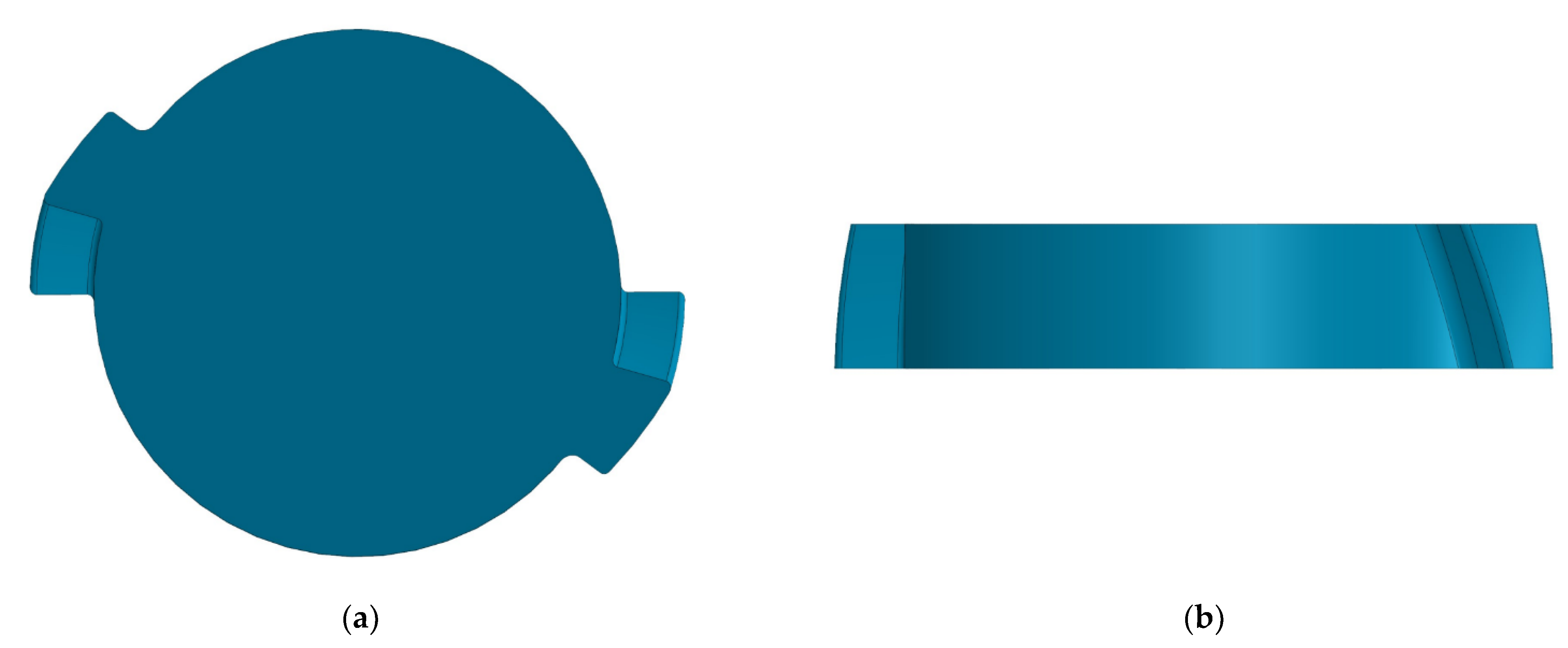
2.1.1. Model of the Micro-Milling Cutter

The model of the micro-milling tool directly affects the simulation accuracy of the micro-milling LF 21 process. The used micro-milling cutter is an MX230 end-milling cutter produced by NS Company in Japan, with a diameter of 0.3 mm. Scanning electron microscopy is used to take images of the tool. The end face and side images of the tool are shown in Figure 1. The images are imported into AutoCAD to copy the end face contour accurately, and a 3D model of the tool is established by rotational stretching according to the end face contour with Pro/E. Then the model is cut and optimized according to the tool geometry parameters obtained from the side images. Figure 2 shows the final result of the 3D geometric model of the micro-milling tool we used in this paper.

Table 1. Geometric parameters of the micro-milling tool.

Geometric Parameter	Symbol	Value
Tool head radius	rc (mm)	0.3
Shank radius	rs (mm)	2
Overall length	L (mm)	45
Extended Length	l (mm)	15
Cutting length	lc (mm)	1.2
Neck taper angle	γ	12°
Helix angle	β	30
Rounded cutting edge radius	r (mm)	0.002
Number of flutes	---	2

shows the geometric parameters of the micro-milling tool.

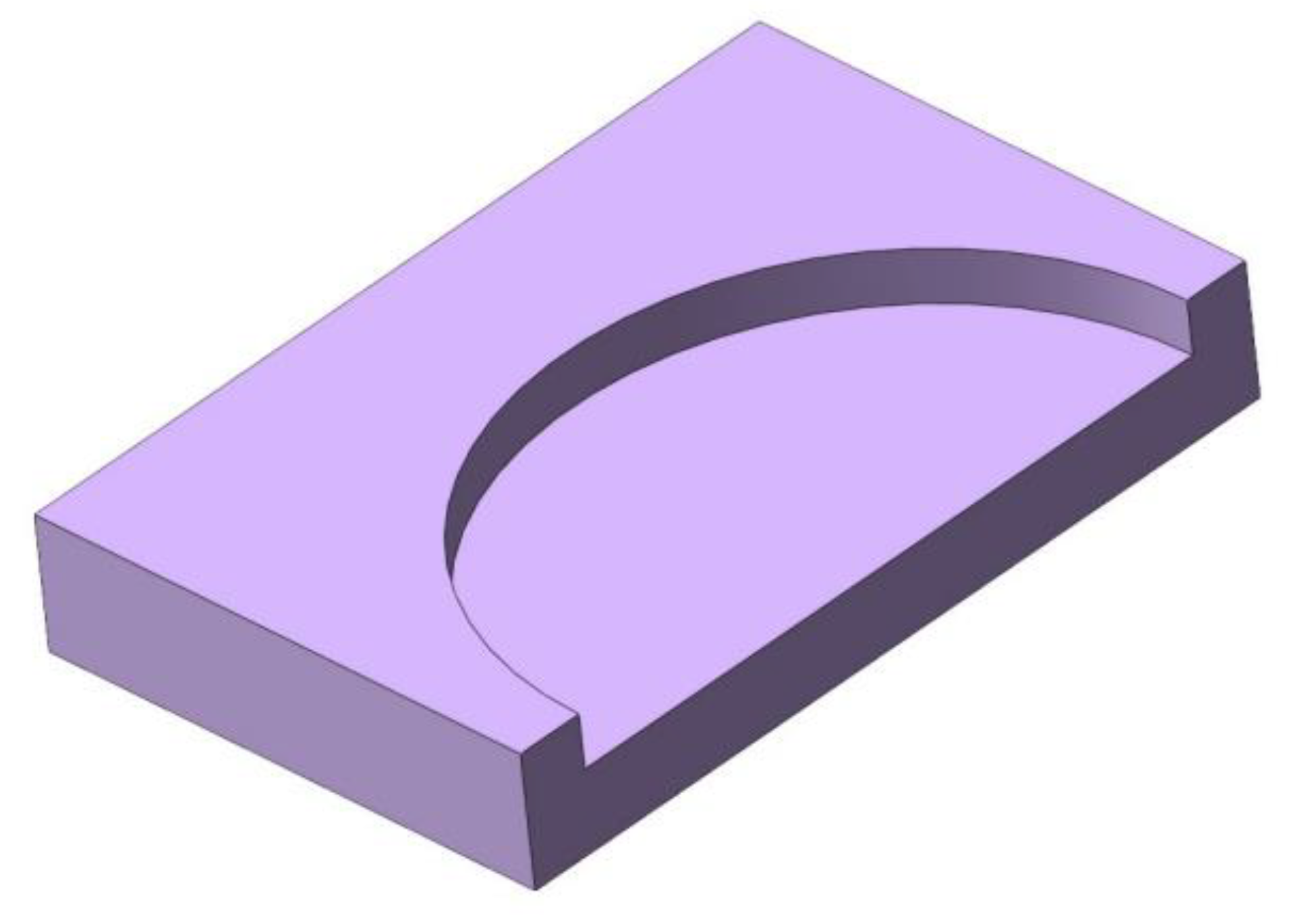
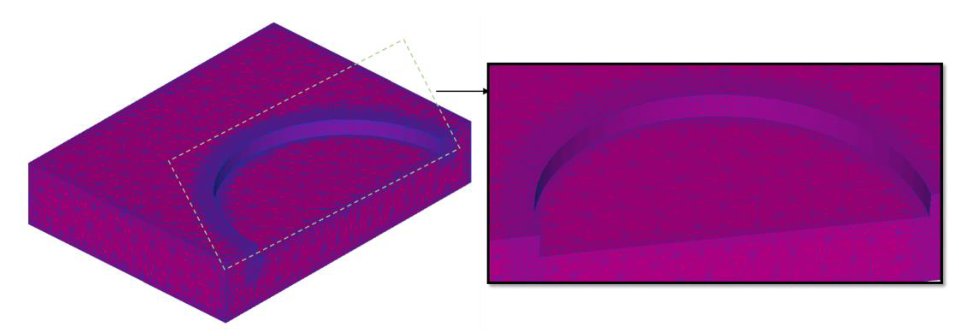
2.1.2. Workpiece Model

The feed per tooth is very small in micro-milling processing; usually is in the tens of micron magnitude. If the workpiece model is established according to the actual size, according to the finite element idea, the minimum mesh of the workpiece should be less than 1/3 of the feed per tooth, which will lead to a large number of mesh and a long calculation time. To raise the calculation efficiency, we intercepted the workpiece model and retained the cutting layer thickness corresponding to the micro-milling cutter radius along the feed direction, as shown in Figure 3.

After the assembly of the model of the micro-milling cutter and workpiece in SolidWorks, the establishment of the geometric model of the simulation is completed in DEFORM 3D.

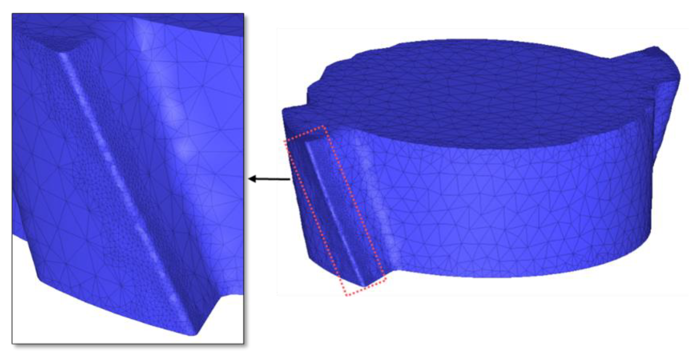
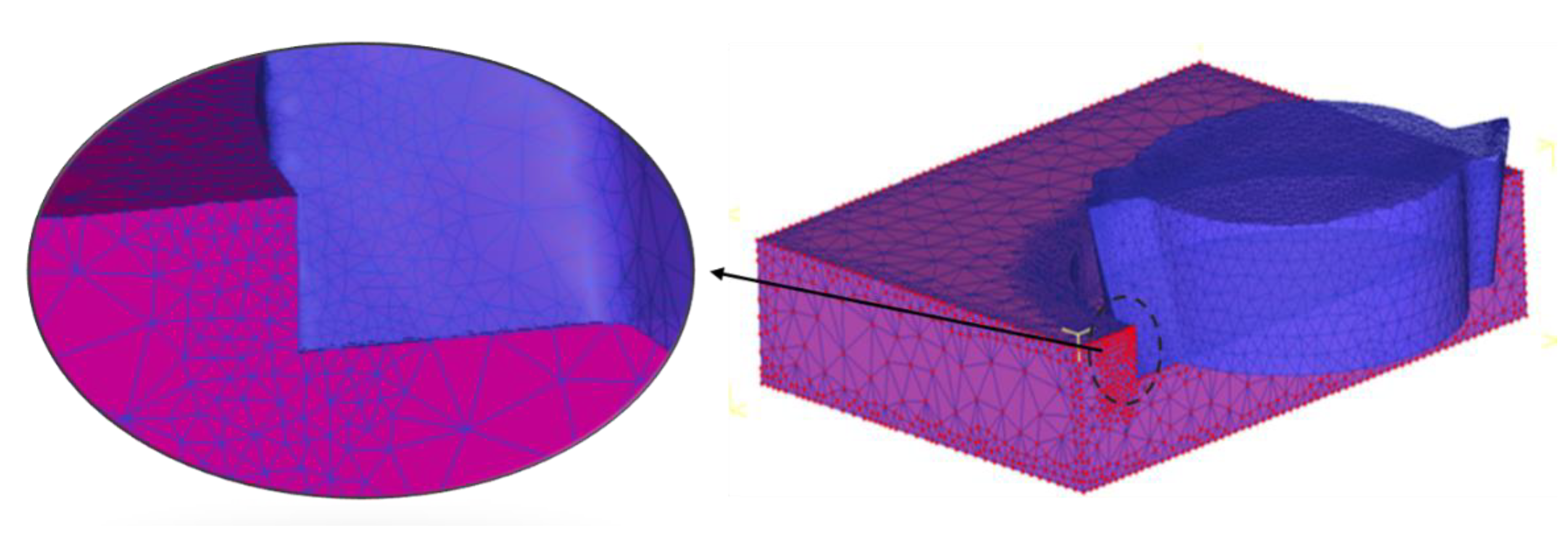
2.2. Material Parameters’ Setting and Meshing

Because the strength and stiffness of the micro-milling cutter are much higher than those of the workpiece, the cutter strain in processing can be ignored, so the micro-milling cutter is regarded as a rigid body; only friction and heat transfer are considered. The micro-milling cutter material is WC/Co, and the coating material is TiAlN. Call the database of material in DEFORM 3D and set the material parameters, as shown in

Table 2. Material parameters of the micro-milling cutter.

Material	Thermal Conductivity (W/(m·°C))	Coefficient of Thermal Expansion (1/°C)	Modulus of Elasticity (Mpa)	Heat Capacity (N/(mm2·°C))	Poisson’s Ratio	Rockwell Hardness
WC/Co (ISO K20)	55	4.7 × 10−6	5.6 × 105	15	0.25	65
TiAlN	12	9.4 × 10−6	6 × 105	15	0.23	83

.

The meshing method of combining relative meshing and local encryption is used, which greatly improves the simulation speed on the premise of ensuring calculation accuracy. The mesh number of the cutter is 50,000, the ratio of the maximum mesh to the minimum mesh is set as 5:1, the local encryption size ratio of the blade is set as 10:1 and the coating thickness is set as 2 μm. The meshing of the micro-milling cutter is shown in Figure 4.

The workpiece material is aluminum alloy LF 21, which belongs to Al-Mn alloy, with low strength, low stiffness and good plasticity. The material parameters of the workpiece are shown in

Table 3. Material parameters of the workpiece.

Material	Thermal Conductivity (W/(m·°C))	Coefficient of Thermal Expansion (1/°C)	Modulus of Elasticity (Mpa)	Heat Capacity (N/(mm2·°C))	Poisson’s Ratio	Brinell Hardness
LF 21 (GB/T3190-1996)	180.2	2.2 × 10−5	6.86 × 104	2.433	0.25	185

.

Because of the characteristics of LF 21, the strain and strain rate of this material are both very high in the process of micro-milling. Therefore, to characterize the material properties and failure criteria of LF 21, the Johnson–Cook constitutive model and failure model are adopted. As shown in Equation (1), is the Johnson–Cook constitutive model [14]:

$$\sigma =[A+B{(\epsilon )}^n][1+C\ln (\frac{\dot{\epsilon }}{{\dot{\epsilon }}_0})][1-{(\frac{T-T_{room}}{T_{melt}-T_{room}})}^m]$$

(1)

where, σ is the stress; A is the yield strength of the material under the reference deformation temperature and the reference strain rate; B is the strain hardening parameter of the material; C is the strain rate coefficient of the material; n is the work hardening parameter of the material; m is the temperature softening parameter of the material; $\dot{\epsilon }$ is the plastic strain rate of the material; ε is the equivalent plastic strain of the material; ${\dot{\epsilon }}_0$ is the reference strain rate of the material; T is the deformation temperature of the material; $T_{room}$ is the room temperature; $T_{melt}$ is the melting temperature of the material. The parameters of the Johnson–Cook constitutive model of aluminum alloy LF 21 are shown in

Table 4. Parameters of Johnson–Cook constitutive model of aluminum alloy LF 21.

Material	A (Mpa)	B (Mpa)	C	n	m	Tmelt (°C)	Troom (°C)
LF 21	34.4	114.2	0.2062	0.2762	0.018	643	20

.

The meshing method of combining relative meshing and local encryption is also used for the meshing of the workpiece. The mesh number is 50,000, the size ratio of the maximum mesh to the minimum mesh is 5:1 and the size ratio of the local encryption of cutting layer is 10:1. Meanwhile, the local encryption area is set to move with the milling cutter, as shown in Figure 5.

2.3. Chip Separation Criterion

Selecting a reasonable chip separation criterion is the key to reflecting chip formation accurately in the actual machining process. Wang Cheng et al. [15] compared the application of Freudenthal, Cockcroft-Latham, Normalized and Ayada fracture criteria to the aluminum alloy cutting process and found that Ayada is most suitable for simulation of cutting aluminum alloy process. So, the Ayada criterion is adopted to simulate the chip generation in micro-milling LF 21 processes:

$$S={\displaystyle {\int }_0^{{\overline{\epsilon }}_f}\frac{{\sigma }_m}{\overline{\sigma }}}d\overline{\epsilon }$$

(2)

where, $S$ is the critical damage value of the material; ${\sigma }_m$ is hydrostatic stress; $\overline{\sigma }$ is equivalent stress; ${\overline{\epsilon }}_f$ is the equivalent plastic strain at fracture; $d\overline{\epsilon }$ is equivalent strain increment. $S$ is set to 0.17 in the simulation.

2.4. Boundary Conditions and Friction Models

In the micro-milling process, the micro-milling cutter rotates at the same time it completes the feed, and the workpiece is fixed on the table. Constrain the non-machined surface of the workpiece, set the Rotation and feed of the cutter and complete the setting of the boundary conditions, as shown in Figure 6. Cutting heat efflux is accomplished by chip, workpiece, cutter and environment diffusion. Set thermal boundary between the workpiece and cutter. The heat transfer coefficient between the cutter and workpiece is set as 107 kW/(m²·K), and the heat transfer coefficient between the environment and the workpiece is set as 45 kW/(m²·K).

The friction regions between the cutter and the workpiece, the cutter and chips are divided into bond zone and slip zone, corresponding to shear friction and Coulomb friction, respectively. The two friction models are shown in Equations (3) and (4), respectively. The contact between the cutter and the workpiece is set as shear friction, and the friction coefficient is set as 0.45. The contact between the workpiece and the chips is set as Coulomb friction, and the friction coefficient is set as 0.2:

$$\mathrm{Shear} \mathrm{friction}: {\tau }_f=\lambda k \mu p_i\ge \lambda k$$

(3)

$$\mathrm{Coulomb} \mathrm{friction}: {\tau }_f=\mu p_i \mu p_i<\lambda k$$

(4)

where, ${\tau }_f$ is frictional stress; $\lambda$ is shear friction coefficient; $k$ is shear yield stress; $\mu$ is Coulomb friction coefficient; $p_{{}_i}$ is the contact surface pressure.

2.5. Constitutive Model of Tool Wear

There are complex friction relations between the cutter, workpiece and chips. To ensure the accuracy of the simulation results of tool wear, it is necessary to select the appropriate constitutive model of tool wear.

The constitutive model of tool wear describes the relationship between cutter volume loss rate and cutting temperature, relative sliding velocity, contact pressure and cutting parameters. Archard and Usui models are provided in DEFORM 3D to calculate the tool wear rate in the cutting process. Usui model can not only study the influence of bond wear on the tool and simulate the crater wear form on the rake face of the cutter but also simulate the flank wear of the cutter [16,17,18]. Usui model is shown in Equation (5):

$$\frac{dW}{dt}=a{\sigma }_n{v}_s{e}^{\raisebox{1ex}{$-b$}\!\left/ \!\raisebox{-1ex}{$T_{\mathrm{c}}$}\right.}$$

(5)

where, $dW/dt$ represents the wear volume of the cutter on a unit area in a unit time; ${\sigma }_n$ represents normal stress; ${\nu }_s$ represents the sliding speed of the workpiece material relative to the cutter; $T_{\mathrm{c}}$ represents the absolute temperature of cutter surface; model constants a and b depend on the material and cutting parameters. The simulation set a to 1 × 10⁻⁷ and b to 850 [19].

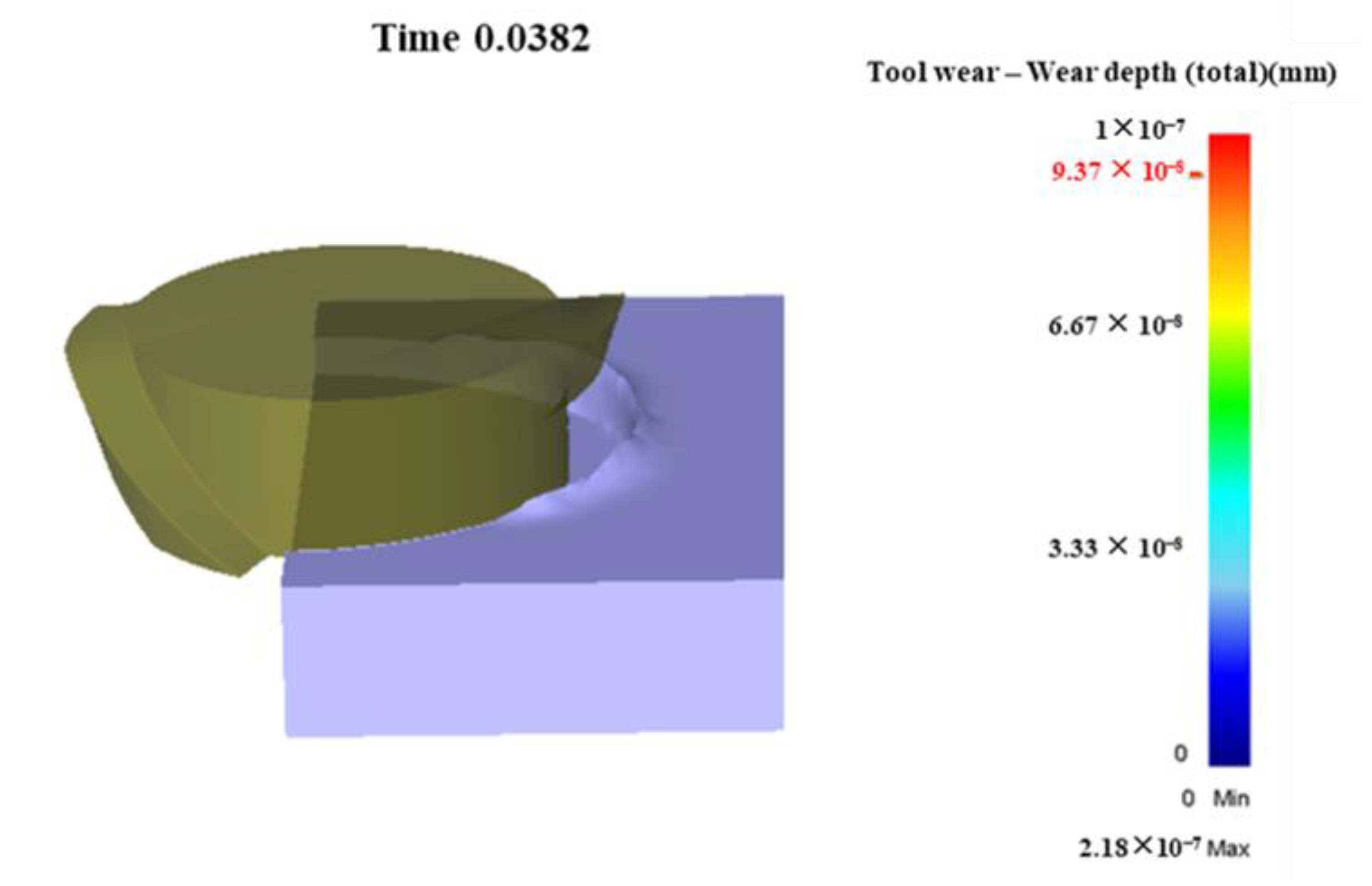
2.6. Prediction of Tool Wear Based on Deform

Deformation and heat transfer are selected in simulation control. Sparse and Newton-Rapnson are selected for solver and iterative methods to ensure convergence under large deformation at the initial stage of simulation. At the later stage of simulation, Conjugate gradient and Newton-Rapnson are adopted to improve solution speed. After the set of the incremental step and simulation time, the set of the preprocessing of the model is finished. Submit the calculation and obtain the cloud map of tool wear depth based on simulation of micro-milling LF 21 processes, as shown in Figure 7.

Assume the tool wear changes linearly with time, and then obtain the cumulative cutter wear depth:

$$W=\frac{\mathsf{\Delta }{W}_{pre}}{\mathsf{\Delta }{t}_{pre}}t$$

(6)

where, $\mathsf{\Delta }{W}_{pre}$ is the tool wear depth output by DEFORM 3D simulation; $\mathsf{\Delta }{t}_{pre}$ is the simulation time; $\mathsf{\Delta }{W}_{pre}/\mathsf{\Delta }{t}_{pre}$ is the average cutter wear rate; $t$ is the cutting time.

DEFORM 3D postprocessing gives the simulation results of the tool wear depth and instantaneous wear rate of any node. However, the tool wear depth cannot be measured directly. Refer to the tool wear evaluation method proposed by Oliaei et al. [20], and use the reduction rate of the tool diameter to characterize the micro-milling tool wear, as shown in Equation (7):

$$\mathrm{Diameter} \mathrm{reduction} \mathrm{rate}\%=\frac{D_{new}-D_{worn}}{D_{new}}\times 100$$

(7)

in which, $D_{new}$ is the diameter of a new cutter; $D_{worn}$ is the diameter of the tool after wear.

Assume the micro-milling tool wear changes linearly with time, that is, the average wear rate of the wool is constant. Figure 8 shows the relationship between tool wear depth and the reduction rate of the tool diameter. Based on the simulated tool wear depth and cutting time, the average tool wear rate can be calculated. The relation between the reduction rate of the tool diameter and tool wear depth at any time is shown in Formula (8):

$$\frac{D_{new}-D_{worn}}{D_{new}}=\frac{D_{new}-2\sqrt{{(D_{new}/2-W\cos (\xi ))}^2+{(W\sin (\xi ))}^2}}{D_{new}}$$

(8)

where, the cumulative tool wear depth is calculated by Equation (6). ξ is the half angle of the cutter tip arc corresponding to the central angle, which is 35°.

According to Figure 8, the relationship between the arc radius of the cutting edge and cumulative tool wear depth can also be obtained, as shown in Equation (9):

$$r_e=\frac{\sin (\xi )}{1-\sin (\xi )}W$$

(9)

where, r_e is the arc radius of the cutting edge; W is the cumulative cutter wear depth.

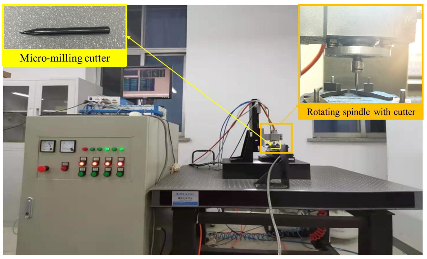
2.7. Experimental Verification of Prediction of Micro-Milling Tool Wear

Experiments of micro-milling aluminum alloy LF 21 are conducted on a micro-milling experimental platform built by our research group earlier (see Figure 9). The spindle speed is between 40,000 rpm and 140,000 rpm. The absolute positioning accuracy of the machine is 1 μm and the repeated positioning accuracy is 0.2 μm. The micro-milling tool used in the experiment is MX230, a two-edge micro-milling tool produced by NS Tool Co., Ltd., Tokyo, Japan, with a diameter of 0.3 mm. The workpiece material is aluminum alloy LF 21, and we selected the VHX-600E super depth of field microscope from KEYENGE to measure the diameter of the micro-milling cutter. The cutting forces corresponding to each set of test parameters are measured using a KISTLER 9256C1 precision 3D force measuring stage. The force meter has three channels, Fx, Fy and Fz, to measure the cutting force in X, Y and Z directions, respectively. Its measurement threshold is only 2 mN, and the measurement range is 250 N. The sampling frequency is 3000 Hz, and the cutting force amplitude can be clearly visualized in the DynoWare software that comes with the charge amplifier KISTLER Type 5080. The comparison of experimental and simulation results of the reduction rate of the tool diameter is shown in

Table 5. The comparison of experimental and simulated reduction rate of the tool diameter.

Number	Spindle Speed n (rpm)	Feed per Tooth fz (μm/z)	Axial Cutting Depth ap (μm)	Cutting Time t (min)	Simulation Output (%)	Experimental Results (%)	Relative Error (%)
1	40,000	0.4	20	4	0.8467	1.1533	26.58
2	40,000	0.6	30	6	2.1133	1.8867	12.01
3	50,000	0.8	20	6	5.7200	8.0333	28.80
4	60,000	0.4	40	6	5.5467	6.7266	17.54
5	60,000	0.8	30	4	10.6400	11.0733	3.91

.

As can be seen from Table 5, the simulated reduction rate of the tool diameter is basically consistent with the experimental measured value, and the average relative error of prediction is 17.77%. The validity of the prediction of tool wear is verified.

3. An Improved Cutting Force Model in Micro-Milling LF 21 Considering Tool Wear

When actual cutting thickness is larger than the minimum cutting thickness during micro-end milling, the cutting layer performs shear slipping plastic deformation under cutting force and is cut away as chips, namely, shear-dominant cutting process. When the actual cutting thickness is smaller than the minimum cutting thickness, the cutting layer, after being ironed by the cutting edge, slips off the flank surface of the tool. Only elastic deformation occurs without any chip, which is called the ploughing-dominant cutting process. When actual cutting thickness is close to the minimum cutting thickness, there will be an accumulation of cutting thickness; thus, the shear-dominant regime and ploughing-dominant regime both exist. Since there is a significant difference between the shear-dominant regime and the ploughing-dominant regime, and only one prediction model cannot describe these two cutting forces [21], the minimum cutting thickness is used as a demarcation point during the micro-end milling process in this paper. The cutting forces prediction model during the shear-dominant cutting process and cutting forces prediction model during the ploughing-dominant cutting process are built, respectively.

3.1. Micro-Milling Force Model

Tool wear will lead to increase in the arc radius of the cutting edge. Sahoo et al. [22] proposed that the friction between the dead zone metal and the cutter tip under the arc radius of the cutting edge should be considered when establishing the force model. Based on the above research results, the authors built a micro-milling force model dominated by shear effects considering tool wear, as shown in Equation (10):

$$\begin{array}{cc}\left\{\begin{array}{l}{F}_x(t)=-(K_{tc}\cdot A_c+K_{tp}\cdot V_c+K_{tw}\cdot {\Phi }_c)-(K_{fc}\cdot A_s+K_{fp}\cdot V_s+K_{fw}\cdot {\Phi }_s)\hfill \\ F_y(t)=(K_{tc}\cdot A_s+K_{tp}\cdot V_s+K_{tw}\cdot {\Phi }_s)-(K_{fc}\cdot A_c+K_{fp}\cdot V_c+K_{fw}\cdot {\Phi }_c)\hfill \\ F_z(t)=(K_{ac}\cdot A_a+K_{ap}\cdot V_a)\hfill \end{array}\right.& t_c>t_{\min }\end{array}$$

(10)

where,

$$\left\{\begin{array}{l}{A}_c=\frac{R}{\sin \phi }{\displaystyle \sum _{k=0}^{K-1}{\displaystyle {\int }_{{\theta }_s}^{{\theta }_e}{t}_c(t,k,\theta )\cos \theta d\theta }}\hfill \\ A_s=\frac{R}{\sin \phi }{\displaystyle \sum _{k=0}^{K-1}{\displaystyle {\int }_{{\theta }_s}^{{\theta }_e}{t}_c(t,k,\theta )\sin \theta d\theta }}\hfill \\ A_a=\frac{R}{\sin \phi }{\displaystyle \sum _{k=0}^{K-1}{\displaystyle {\int }_{{\theta }_s}^{{\theta }_e}{t}_c(t,k,\theta )d\theta }}\hfill \end{array}\right.$$

(11)

$$\left\{\begin{array}{l}{V}_c=\frac{R}{\sin \phi }{\displaystyle \sum _{k=0}^{K-1}{\displaystyle {\int }_{{\theta }_s}^{{\theta }_e}{A}_p\cos \theta d\theta }}\hfill \\ V_s=\frac{R}{\sin \phi }{\displaystyle \sum _{k=0}^{K-1}{\displaystyle {\int }_{{\theta }_s}^{{\theta }_e}{A}_p\sin \theta d\theta }}\hfill \\ V_a=\frac{R}{\sin \phi }{\displaystyle \sum _{k=0}^{K-1}{\displaystyle {\int }_{{\theta }_s}^{{\theta }_e}{A}_{p}d\theta }}\hfill \end{array}\right.$$

(12)

$$\left\{\begin{array}{c}{\Phi }_c=\frac{R}{\sin \phi }{\displaystyle \sum _{k=0}^{K-1}{\displaystyle {\int }_{{\theta }_s}^{{\theta }_e}\cos \theta d\theta }}\\ {\Phi }_s=\frac{R}{\sin \phi }{\displaystyle \sum _{k=0}^{K-1}{\displaystyle {\int }_{{\theta }_s}^{{\theta }_e}\sin \theta d\theta }}\end{array}\right.$$

(13)

$F_x(t)$, $F_y(t)$ and $F_z(t)$ are the components of cutting force decomposition to $x$, $y$ and $z$ directions. $K_{fc}$, $K_{tc}$ and $K_{ac}$ are radial, tangential and axial shear force coefficients, respectively. The coefficients of plough force $K_{fp}$, $K_{tp}$ and $K_{ap}$ are radial, tangential and axial, respectively. $K_{fw}$ and $K_{tw}$ are radial and tangential friction coefficients, respectively. $t_c(t,k,z)$ is the instantaneous cutting thickness of the $k$ cutting edge at the axial position $z$ at time $t$. $A_p$ is the area of plough area. $t_{\min }$ is the minimum cutting thickness. $\theta$ is the tooth angle. ${\theta }_s$ and ${\theta }_e$ are the limit cutting-in and cutting-out angles, respectively. $R$ is the radius of the micro-milling cutter. $k$ is the number of cutter tooth. $K$ is the total number of cutter tooth.

As shown in Figure 10, the shaded area is the area of the plough area when the actual cutting thickness is less than the minimum cutting thickness. Taking the maximum elastic recovery $\delta$ as the node, the plough area is solved in two cases, respectively.

The plough area $A_p$ is calculated as follows:

$$A_p=\frac{1}{2}{r}_e^2({\alpha }_S+{\alpha }_0)+\frac{1}{2}{r}_e\cdot l_{AB}-\frac{1}{2}{r}_e\cdot l_{BO}\cdot \sin ({\alpha }_S+{\alpha }_0+{\alpha }_P)$$

(14)

where, ${\alpha }_0$ is the back edge angle; $r_e$ is the radius of the cutting edge arc; $\delta$ is the elastic recovery of material.

$${\alpha }_S={\cos }^{-1}\left(\frac{r_e-t_{\min }}{r_e}\right)$$

(15)

$${\alpha }_P={\tan }^{-1}\left(\frac{l_{AB}}{r_e}\right)$$

(16)

$$l_{AB}=\frac{\delta -r_e(1-\cos {\alpha }_0)}{\sin {\alpha }_0}$$

(17)

$$l_{BO}=\sqrt{r_e{}^2+l_{AB}{}^2}$$

(18)

Material elastic recovery δ is calculated as Equation (19):

$$\delta ={\delta }_{\max }=\frac{3\cdot {\sigma }_s}{4\cdot E}\cdot r_e\cdot \left[2\exp \left(\frac{H}{{\sigma }_s}-\frac{1}{2}\right)-1\right]$$

(19)

where, ${\sigma }_s$ is tensile strength; $E$ is elastic modulus; $H$ is hardness.

The limit cutting and cutting angles ${\theta }_s$ and ${\theta }_e$ are shown in Formulas (20) and (21), respectively:

$${\theta }_s=0$$

(20)

$${\theta }_e=\pi$$

(21)

The authors also built a micro-milling force model dominated by plough effect, as shown in Equation (22):

$$\begin{array}{cc}\left\{\begin{array}{c}{F}_x(t)=-(K_{tpp}\cdot V_c+K_{tw}\cdot {\Phi }_c)-(K_{fpp}\cdot V_s+K_{fw}\cdot {\Phi }_s)\hfill \\ F_y(t)=(K_{tpp}\cdot V_s+K_{tw}\cdot {\Phi }_s)-(K_{fpp}\cdot V_c+K_{fw}\cdot {\Phi }_c)\hfill \\ F_z(t)=K_{ap}\cdot V_a\hfill \end{array}\right.& t_c\le t_{\min }\end{array}$$

(22)

where, $K_{fpp}$, $K_{tpp}$ and $K_{app}$ are coefficients of radial, tangential and axial plow force, respectively, and other parameters are similar to Equation (10).

The maximum elastic recovery ${\delta }_{\max }$ of the material is calculated as follows:

$${\delta }_{\max }=\frac{3\cdot {\sigma }_s}{4\cdot E}\cdot r_e\cdot \left[2\exp \left(\frac{H}{{\sigma }_s}-\frac{1}{2}\right)-1\right]$$

(23)

Calculation of plough area $A_p$ is slightly complicated and is divided into two cases as follows:

• If $t_c>{\delta }_{\max }$, the plough area can be calculated as Formula (24):

$$A_p=\frac{1}{2}{r}_e^2({\alpha }_C+{\alpha }_0)+\frac{1}{2}{r}_e\cdot l_{AB}-\frac{1}{2}{r}_e\cdot l_{BO}\cdot \sin ({\alpha }_C+{\alpha }_0+{\alpha }_P)$$

(24)

where,

$${\alpha }_C={\cos }^{-1}\left(\frac{r_e-t_c}{r_e}\right)$$

(25)

$${\alpha }_P={\tan }^{-1}\left(\frac{l_{AB}}{r_e}\right)$$

(26)

$$l_{AB}=\frac{{\delta }_{\max }-r_e(1-\cos {\alpha }_0)}{\sin {\alpha }_0}$$

(27)

$$l_{BO}=\sqrt{r_e{}^2+l_{AB}{}^2}$$

(28)

2.

If $t_c\le {\delta }_{\max }$, the plough area is calculated as follows:

$$A_p=\frac{1}{2}{r}_e^2({\alpha }_D+{\alpha }_0)+\frac{1}{2}{r}_e\cdot l_{AE}-\frac{1}{2}{r}_e\cdot l_{EO}\cdot \sin ({\alpha }_D+{\alpha }_0+{\alpha }_{Pe})$$

(29)

where,

$${\alpha }_D={\cos }^{-1}\left(\frac{r_e-t_c}{r_e}\right)$$

(30)

$${\alpha }_{Pe}={\tan }^{-1}\left(\frac{l_{AE}}{r_e}\right)$$

(31)

$$l_{AE}=\frac{t_c-r_e(1-\cos {\alpha }_0)}{\sin {\alpha }_0}$$

(32)

$$l_{EO}=\sqrt{r_e{}^2+l_{AE}{}^2}$$

(33)

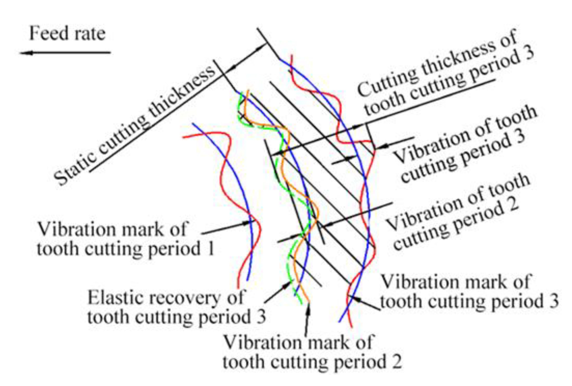
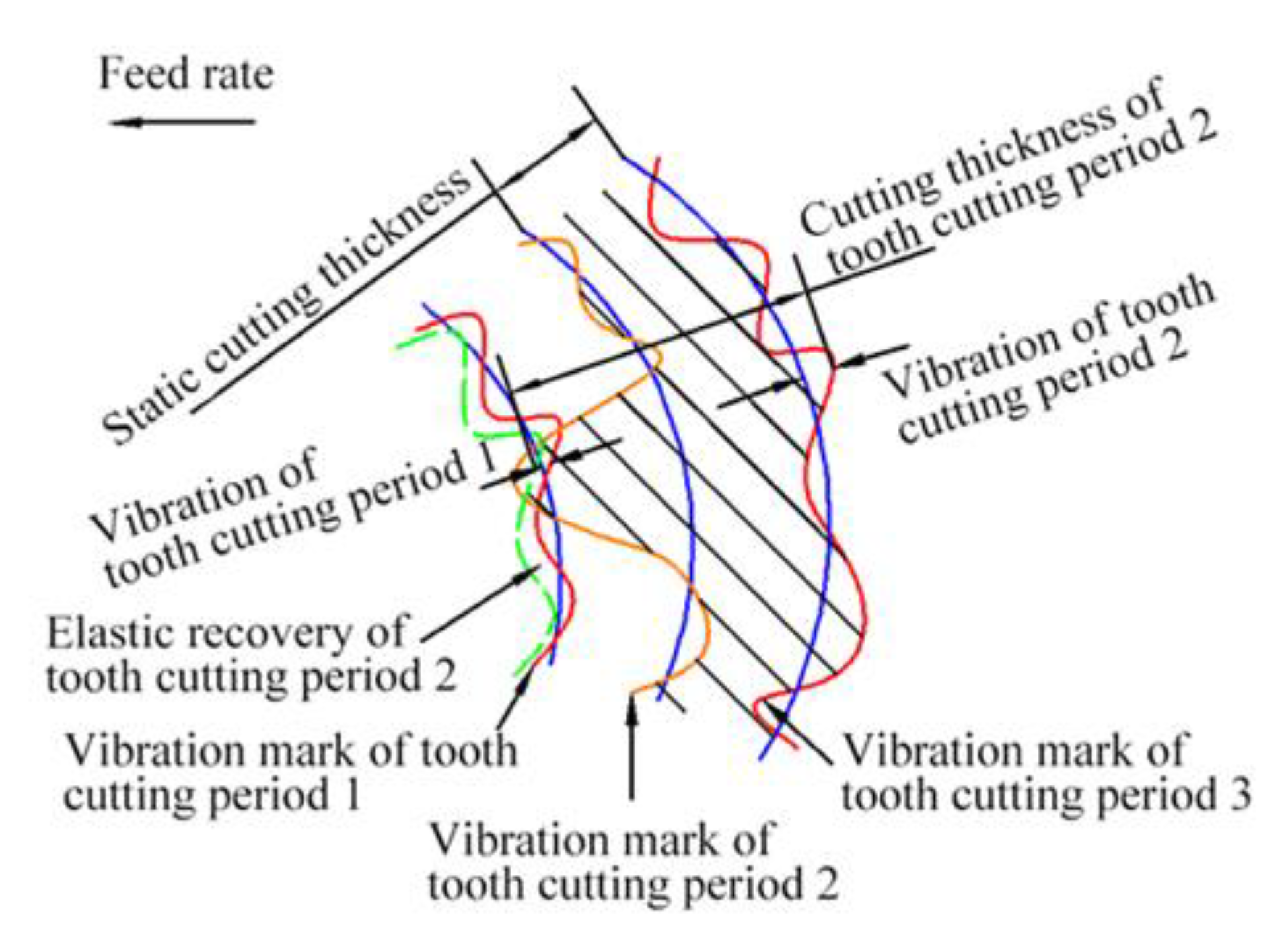
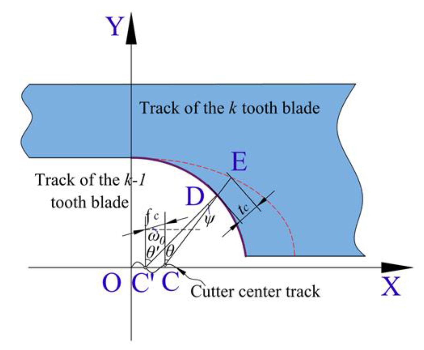
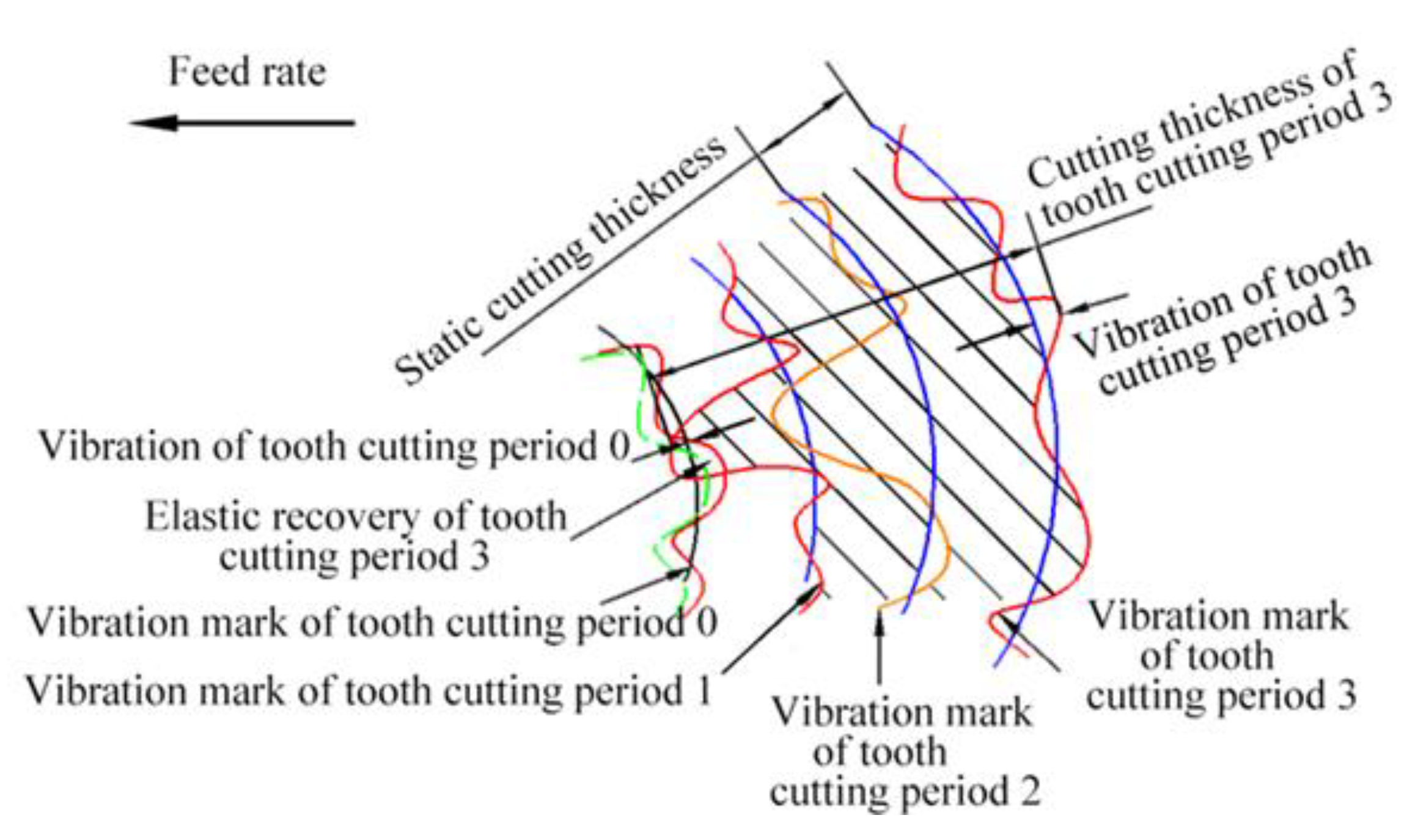
3.2. Instantaneous Cutting Thickness Model

The calculation of instantaneous cutting thickness is the basis of the solving force model. Li Guangjun [23] established an analytical model of instantaneous cumulative cutting thickness; however, the iterative solution requires a lot of computation. According to the actual cutting trajectory of the cutter, Nie Qiang et al. [24] built an instantaneous cutting thickness model considering the cutter runout by using microscopic geometric relations and obtained approximate solutions through Taylor series expansion. In this paper, based on the above modeling experience, an instantaneous cutting thickness model of micro-milling is established considering the cutter runout, the minimum cutting thickness, material elastic recovery and cutter vibration displacement, as shown in Figure 11.

The instantaneous cutting thickness model considering cutter runout is calculated using Equation (34):

$$t_c(k)=f_z(1-\frac{\psi }{\pi })\sin {\theta }_k+2R_t\cos {\phi }_k-R_t\psi \sin {\phi }_k+R\frac{{\psi }^2}{2}$$

(34)

where, ${\theta }_k=\theta +\pi (k-1)$, θ is the tooth angle; ${\phi }_k={\phi }_0-\pi (k-1)$, ${\phi }_0$ is the cutter run-out angle, which is 45°; $\psi =(f_z\cos {\theta }_k+2R_t\sin {\phi }_k)/(R+f_z\cos {\theta }_k/\pi -R_t\cos {\phi }_k)$.

When $2R_t\cos {\phi }_k>f_z$, single tooth cutting phenomenon occurs. If $k-1$ tooth is truncated, the cutting thickness of $k$ tooth needs to be corrected, as shown in Equation (35).

$$t_c{(k)}_{\mathrm{mod}}=t_c(k)+t_c(k-1)$$

(35)

Because the processing scale is greatly reduced, the plough effect cannot be ignored. The plough effect causes elastic recovery of materials, and elastic recovery of materials is calculated using Equation (36).

$$\left\{\begin{array}{ll}\delta (k-1)={\delta }_{\max }=\frac{3\cdot {\sigma }_s}{4\cdot E}\cdot r_e\cdot \left[2\exp \left(\frac{H}{{\sigma }_s}-\frac{1}{2}\right)-1\right]\hfill & t_c(k-1)>{\delta }_{\max }\hfill \\ \delta (k-1)=t_c(k-1) \hfill & t_c(k-1)\le {\delta }_{\max }\hfill \end{array}\right.$$

(36)

If the elastic recovery of the $k-1$ tooth workpiece material is $\delta (k-1)$, the cutting thickness of the $k$ tooth needs to be modified, as shown in Equation (37).

$$t_c{(k)}_{\mathrm{mod}}=t_c(k)+\delta (k-1)$$

(37)

Under the excitation of micro-milling force, there exists relative vibration between the micro-milling cutter and the workpiece, which makes the actual cutting path of the cutter deviates from the theoretical cutting path. Vibration affects the instantaneous cutting thickness. The instantaneous cutting thickness model considering the cutter vibration displacement is divided into two cases:

• The blade does not run out of the cutting;

Instantaneous cutting thickness in the milling process is shown in Figure 12. The cutter tooth immerses in the workpiece in tooth cutting period 2. Chatter mark is left on workpiece surface. The chatter mark in tooth cutting period 3 is corresponding to chatter mark in tooth cutting period 2. On the aspect of machined surface elastic recovery, in fact, machined surface elastic recovery caused in tooth cutting period 2 increases instantaneous cutting thickness in tooth cutting period 3. That is because machined surface elastic recovery caused in tooth cutting period 2 occurs after cutting. The effects of vibration and machined surface elastic recovery are independent. As a result, the instantaneous cutting thickness in tooth cutting period 3 should be:

$$t_c{(3)}_{\mathrm{mod}}=t_c(3)+(v_2-v_3)$$

(38)

where, $v_2$ and $v_3$ represent vibration displacement corresponding to tooth cutting period 2 and 3, respectively.

2.

Cutter tooth loses contact with the workpiece.

It is assumed that the cutter tooth immerses in the workpiece in tooth cutting period 1. Instantaneous cutting thickness in the milling process is shown in Figure 13. The cutter tooth loses contact with the workpiece in tooth cutting period 2. Chatter mark is not left on workpiece surface. The nearest to the chatter mark in tooth cutting period 3 is the mark left in tooth cutting period 1. Because cutting does not occur in tooth cutting period 2, static cutting thickness resulting from feed per tooth in period 2 is not yet removed and needs to be removed in tooth cutting period 3. On the aspect of machined surface elastic recovery, because cutting does not occur in tooth cutting period 2, machined surface elastic recovery layer in tooth cutting period 3 is from tooth cutting period 1. Therefore, the instantaneous cutting thickness in tooth cutting period 3 should be:

$$t_c{(3)}_{\mathrm{mod}}=t_c(3)+t_c(2)+(v_1-v_3)$$

(39)

Due to the excessive vibration displacement of the cutter tooth, it may temporarily run out of the cutting phenomenon. So, the instantaneous cutting thickness of the current period is not only affected by the last period but may be affected by the previous period or even earlier period, which is the multiple regeneration effect. For example, two consecutive cutter teeth run out simultaneously at a certain tooth angle, as shown in Figure 14. Both tooth cutting period 1 and tooth cutting period 2 run out of cutting due to excessive vibration displacement. The instantaneous cutting thickness of tooth cutting period 3 depends on the theoretical instantaneous cutting thickness between tooth cutting period 0 and tooth cutting period 3 and the corresponding vibration displacement of tooth cutting period 0 and tooth cutting period 3, as shown in Equation (40):

$$t_c{(3)}_{\mathrm{mod}}=t_c(3)+t_c(2)+t_c(1)+\delta (0)+(v_0-v_3)$$

(40)

Therefore, the effects that the cutter tooth loses contact with workpiece and multiple regeneration can be taken into consideration by recurrence relation between two adjacent tooth cutting periods. It is ensured that chatter mark in previous period is the nearest to the mark in current tooth cutting period. Thus, the model of instantaneous cutting thickness considering multiple regeneration effects is expressed by the following formulas:

$$t_c{(k)}_{\mathrm{mod}}=t_c(k)+(v_{k-1}-v_k)+hp{r}_k$$

(41)

where, $v_{k-1}$ and $v_k$ are vibration patterns corresponding to the instantaneous cutting thickness of the $k-1$ edge and the $k$ edge, respectively, and the recursive formula of $v_{k-1}$ is shown in Equation (42). $hp{r}_k$ is the cutting thickness compensation of $k$ the edge, and its recursive formula is shown in Equation (43).

$$\left\{\begin{array}{cc}{v}_{k-1}=v_{k-1}& t_c(k-1)>0\\ v_{k-1}=v_{k-2}& t_c(k-1)\le 0\end{array}\right.$$

(42)

$$\left\{\begin{array}{ll}hp{r}_k={\delta }_{k-1}\hfill & t_c(k-1)>0\hfill \\ hp{r}_k=t_c(k-1)+hp{r}_{k-1}\hfill & t_c(k-1)\le 0\hfill \end{array}\right.$$

(43)

3.3. Parameter Identification of the Micro-Milling Force Model

The minimum cutting thickness is used as a demarcation point to build the micro- milling force model. The research group has found that the micro-milling force increases significantly near the minimum cutting thickness. We conduct several experiments, and the experimental results are shown in

Table 6. Experiments for determining the minimum cutting thickness.

Number	Spindle Speed n (rpm)	Axial Cutting Depth ap (μm)	Feed per Tooth fz (μm/z)	Fx (N)	Fy (N)	Fz(N)
1	40,000	50	0.25	0.0735	0.5045	0.2857
2	40,000	50	0.35	0.0936	0.6645	0.2886
3	40,000	50	0.45	0.1246	0.7894	0.3306
4	40,000	50	0.55	0.1043	0.6275	0.2882
5	40,000	50	0.65	0.1223	0.7293	0.3245

. Based on the experimental results, we determine that the minimum cutting thickness of micro-milling aluminum alloy LF 21 is 0.45 μm.

There are altogether eleven coefficients in the cutting force model, as shown in Equations (10) and (22). Coefficient of shear effect indicates cutting force that the cutting edge infinitesimal withstands when cutting chip per unit cutting layer area. Ploughing effect coefficient indicates cutting force that the cutting edge infinitesimal withstands when there is unit interference volume between the cutting edge infinitesimal and machined surface. Cutting force coefficients are related to geometrical parameters of tools, materials of tools and materials of workpiece. For different tool materials and workpiece materials, cutting force coefficients are different, and thus, it is necessary to conduct parameter identification before utilizing cutting force prediction model. The cutting force coefficients are determined based on experiments.

To determine the coefficients of micro-milling force model dominated by shear and plough effects, the authors refer to the research method of the literature [23]. By solving the cutting layer area and interference volume of the cutting edge at a certain tooth angle, combing the experimental force data and using the least square method, we obtain the coefficients of the force model.

The cutting layer area corresponding to different tooth angles of the cutting edge involved in cutting is decomposed to the $\mathrm{x}-\mathrm{y}$ coordinate axis. The simulation curve of the cutter rotation is shown in Figure 15. The simulation conditions are as follows: n = 40,000 rpm, a_p = 20 μm and f_z = 0.8 μm/z.

Figure 15 indicates that when the tooth angle at the bottom of the micro-milling cutter-edge line is 2.356 radians, the cutting layer area decomposed along the y axis reaches the maximum, corresponding to the peak of the cutting force in the y-direction. When the tooth angle at the bottom of the micro-milling cutter-edge line is 1.571 radians, the cutting layer area decomposed along the x axis reaches the peak.

According to cutting forces prediction model of Formula (10), $A_c$ and $A_s$ corresponding to the tooth part involved in cutting at different tooth angles are solved. The simulation curve of cutter rotation is shown in Figure 16. The maximum cutting force in $y$ direction corresponds to the tooth angle at the bottom of the blade at 2.356 radians. Where, $A_{cy}=-3.0261\times {10}^{-11}{\mathrm{m}}^2$,$A_{sy}=3.1236\times {10}^{-11}{\mathrm{m}}^2$. Similarly, the peak x-direction cutting force corresponds to the tooth angle at the bottom of the blade at 1.571 radians. Where, $A_{cx}=2.5578\times {10}^{-12}{\mathrm{m}}^2$, $A_{sx}=5.8777\times {10}^{-11}{\mathrm{m}}^2$.

The $V_c$ and $V_s$ corresponding to the tooth involved in cutting at different tooth angles can be solved according to the cutting force model. The simulation curve of the cutter rotation is shown in Figure 17. The peak cutting force in y-direction corresponds to the tooth angle of the end of the blade bottom at 2.379 radians. Where, $V_{cy}=-4.1442\times {10}^{-18}{\mathrm{m}}^3$, $V_{sy}=4.2738\times {10}^{-18}{\mathrm{m}}^3$. Similarly, the peak value of x-direction cutting force corresponds to the tooth angle at the bottom of the blade at 1.566 radian. Where, $V_{cx}=2.5790\times {10}^{-19}{\mathrm{m}}^3$, $V_{sx}=5.9234\times {10}^{-18}{\mathrm{m}}^3$.

Assume that the maximum cutting layer area corresponds to the axial force peak value. Figure 18 shows the results obtained from the studies of maximum cutting layer area corresponds to the z-direction cutting force peak value when the tooth angle at the bottom of the blade is 1.6085 radian. Where, $A_a=5.8904\times {10}^{-11}{\mathrm{m}}^2$, $V_a=5.9305\times {10}^{-18}{\mathrm{m}}^3$.

The experimental design and results of determination of coefficients of micro-milling force model dominated by shear effect are shown in

Table 7. Determination of coefficients of micro-milling force model dominated by shear effect.

Number	Spindle Speed n (rpm)	Axial Cutting Depth ap (μm)	Feed per Tooth fz (μm/z)	Fx (N)	Fy (N)	Fz (N)
1	40,000	20	0.8	0.0805	0.1463	0.0555
2	45,000	30	0.8	0.0709	0.1347	0.0873
3	50,000	40	0.8	0.2571	0.3071	0.1731
4	55,000	50	0.8	0.3391	0.3513	0.1365
5	60,000	60	0.8	0.1099	0.1525	0.1581
6	40,000	30	0.9	0.1615	0.1660	0.2272
7	45,000	40	0.9	0.1087	0.1747	0.0918
8	50,000	50	0.9	0.1956	0.2987	0.2336
9	55,000	60	0.9	0.1235	0.1983	0.1772
10	60,000	20	0.9	0.0643	0.1255	0.1262
11	40,000	40	1.0	0.0961	0.1436	0.1024
12	45,000	50	1.0	0.2109	0.2749	0.1736
13	50,000	60	1.0	0.2354	0.3033	0.1647
14	55,000	20	1.0	0.1365	0.2457	0.1215
15	60,000	30	1.0	0.0930	0.1271	0.1569

.

Coefficients $A_c$, $A_s$, $V_c$ and $V_s$ of the force model dominated by shear effect are solved, respectively, by the least square method. K_tc = −6.43155 × 108, K_tp = 4.53989 × 1016, K_fc = 2.00831 × 108, K_fp = −1.94050 × 1016, K_ac = 2.37296 × 108 and K_ap = 6.39313 × 1015.

Similarly, the experimental results of determination of coefficients of micro-milling force model dominated by plough effect are shown in

Table 8. Determination of coefficients of micro-milling force model dominated by plough effect.

Number	Spindle Speed n (rpm)	Axial Cutting Depth ap (μm)	Feed per Tooth fz (μm/z)	Fx (N)	Fy (N)	Fz (N)
1	40,000	20	0.2	0.0767	0.1737	0.0841
2	45,000	30	0.2	0.0262	0.0585	0.0449
3	50,000	40	0.2	0.0545	0.1681	0.0746
4	55,000	50	0.2	0.1957	0.4321	0.1539
5	60,000	60	0.2	0.1391	0.2261	0.1705
6	40,000	30	0.3	0.0743	0.3581	0.2091
7	45,000	40	0.3	0.0875	0.1347	0.0868
8	50,000	50	0.3	0.1342	0.2791	0.1925
9	55,000	60	0.3	0.3232	0.6032	0.2945
10	60,000	20	0.3	0.0550	0.1371	0.1159
11	40,000	40	0.4	0.0939	0.4853	0.2541
12	45,000	50	0.4	0.2612	0.3766	0.1114
13	50,000	60	0.4	0.2335	0.4019	0.1566
14	55,000	20	0.4	0.0814	0.2525	0.1713
15	60,000	30	0.4	0.0880	0.2173	0.1249

.

The least square method is also used to estimate the coefficients of the force model dominated by plough effect, and the values of $V_c$ and $V_s$ are successively solved where, K_tpp = 4.03217 × 1016, K_fpp = −1.06732 × 1016 and K_app = 1.18242 × 1016.

3.4. Micro-Milling Force Model Considering Tool Wear

As the cutting process goes on, the arc radius of the cutting edge increases, the friction between the cutter and the workpiece also increases, which will lead to the increase in micro-milling force. Therefore, the influence of tool wear should be considered when building force model. As the radius of the tool tip arc increases, a small, stable chip will exist between the tool tip arc and the workpiece and accumulate at this location for a long time, forming a built-up edge, hypothetically an ideal rigid plastic material, which is called the metal dead zone [25]. Part of the workpiece material in the dead zone flow out as chips along the rack face of the cutter, and the other part extrudes and rubs with cutter and remains on the surface, as shown in Figure 19. We propose a model of force coefficients mainly caused by the increase in arc radius of the cutting edge considering cutting dead zone, as shown in Equation (44):

$$\left\{\begin{array}{l}{K}_{tw}=\tau r_e(\pi \sin {\theta }_1\tan {\theta }_1+\frac{2{\theta }_1}{\cos {\theta }_1})\hfill \\ K_{fw}=\tau r_e(2\sqrt{3}\sin {\theta }_1)\hfill \end{array}\right.$$

(44)

where, K_tw and K_fw are the coefficients of tangential and normal force in the friction action caused by the increase in the arc radius of the cutting edge. r_e is arc radius of the cutting edge; θ₁ is the stagnation angle, which is 14°. τ is the shear stress of materials. The additional friction force caused by tool wear can be expressed as:

$$\left\{\begin{array}{l}{F}_x(t)=-(K_{tw}\cdot {\Phi }_c)-(K_{fw}\cdot {\Phi }_s)\hfill \\ F_y(t)=(K_{tw}\cdot {\Phi }_s)-(K_{fw}\cdot {\Phi }_c)\hfill \\ F_z(t)=0\hfill \end{array}\right.$$

(45)

in which:

$$\left\{\begin{array}{c}{\Phi }_c=\frac{R}{\sin \phi }{\displaystyle \sum _{k=0}^{K-1}{\displaystyle {\int }_{{\theta }_s}^{{\theta }_e}\cos \theta d\theta }}\\ {\Phi }_s=\frac{R}{\sin \phi }{\displaystyle \sum _{k=0}^{K-1}{\displaystyle {\int }_{{\theta }_s}^{{\theta }_e}\sin \theta d\theta }}\end{array}\right.$$

(46)

The validity of the built force model considering tool wear in micro-end milling of LF 21 process is testified by micro-slot milling experiments. Cutting parameters are as follows: n = 40,000 rpm, ap = 20 μm and fz = 0.8 μm/z. The prediction curve of micro-milling force considering tool wear and the force curve measured in experiments are shown in Figure 20.

Figure 20 shows that the predicted peak values of micro-milling forces in X, Y and Z directions are basically consistent with the experimental results, and the changing rules of cutting force are essentially identical. Whereas the predicted results of X cutting force are generally greater than the experimental measured values. There exist primary and secondary peak forces in a cutting cycle. It is verified that the phenomenon of uneven loading of two teeth happens because of the cutter runout in micro-milling process. It is proved that the built micro-milling force model of aluminum alloy LF 21 is effective.

4. Conclusions

By considering the aforesaid tool wear and cutting force modeling, conclusions can be drawn as follows:

• A simulation model based on DEFORM 3D is built to simulate the process of micro-milling aluminum alloy LF 21 and the prediction of tool wear is achieved. The results proved that the Usui wear rate model can effectively predict the tool wear in the micro-milling process.
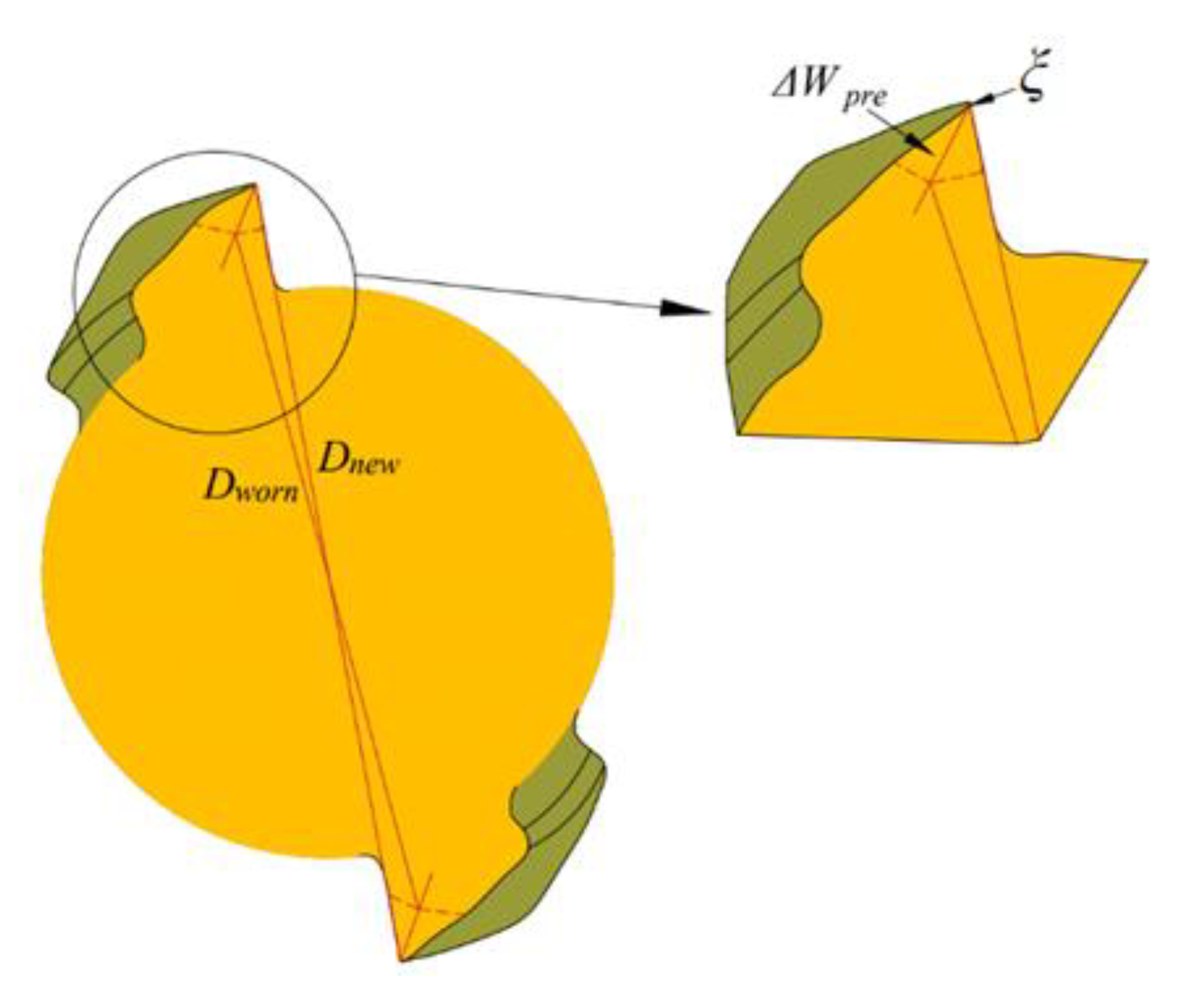
• The arc radius of the cutting edge increases due to tool wear; the friction between the cutter and the workpiece also increases. In this paper, the average tool wear rate is used to solve the cutting edge arc radius dynamically. In addition, considering the effects of tool run-out, material elastic recovery and cutter vibration displacement, the instantaneous cutting thickness model is established.
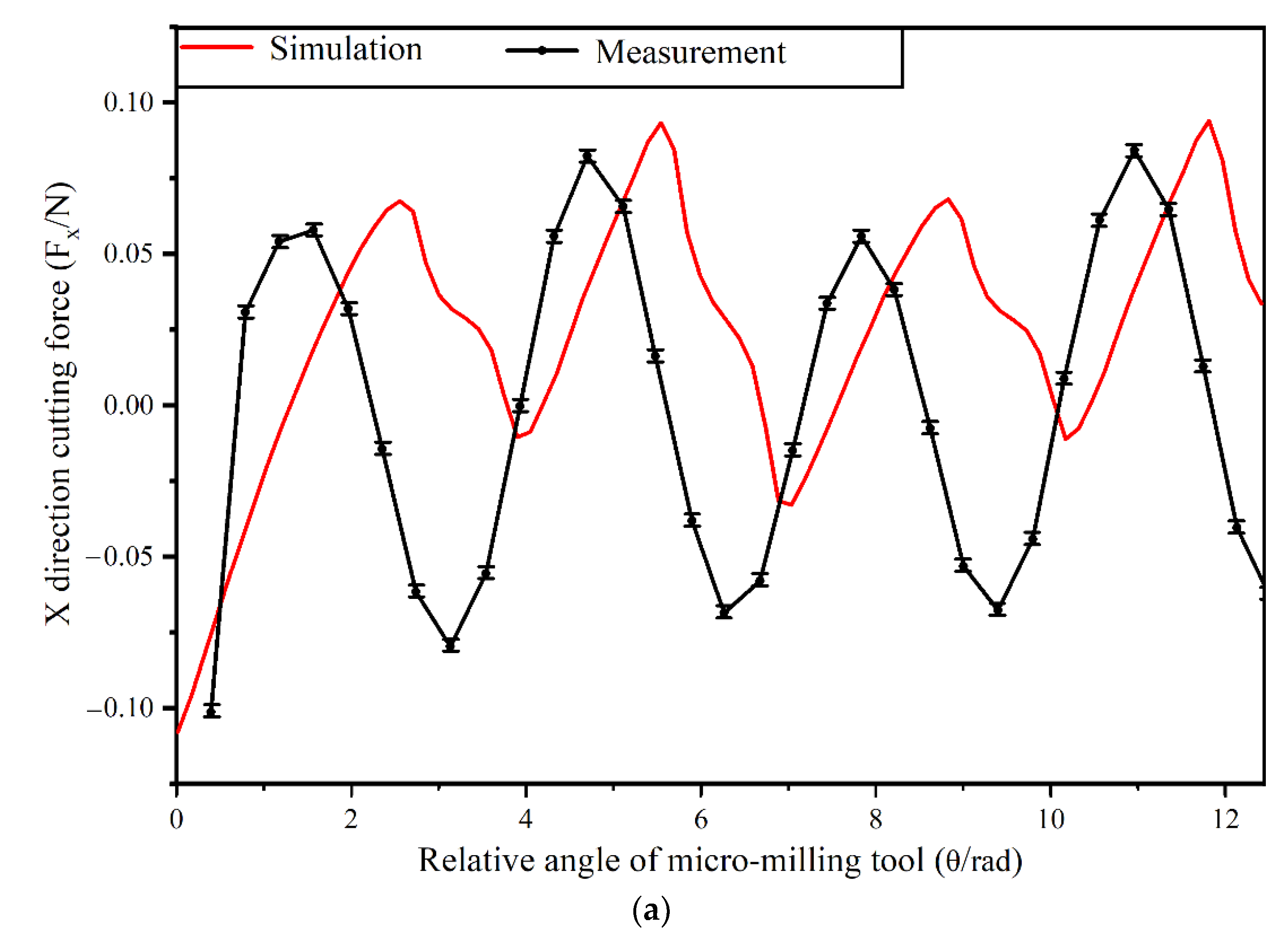
• Based on the instantaneous cutting thickness and minimum cutting thickness values, we established the force model of aluminum alloy LF 21 micro-milling process based on shear effect and plough effect and verified the validity of the force model by experiment.
• We also propose a model of force coefficients mainly caused by the increase in arc radius of the cutting edge considering cutting dead zone. The experiment results verify that the cutting forces prediction results and experiment results are well matched.

References

1. Thepsonthi, T.; Özel, T. 3-D finite element process simulation of micro-end milling ti-6al-4v titanium alloy: Experimental validations on chip flow and cutter wear. J. Mater. Process. Technol. 2015, 221, 128–145. [Google Scholar] [CrossRef]
2. Thepsonthi, T.; Özel, T. Experimental and finite element simulation based investigations on micro-milling ti-6al-4v titanium alloy: Effects of cbn coating on cutter wear. J. Mater. Process. Technol. 2013, 213, 532–542. [Google Scholar] [CrossRef]
3. Lu, X.H.; Wang, F.R.; Jia, Z.Y.; Liang, S.Y. The flank wear prediction in micro-milling inconel 718. Ind. Lubr. Tribol. 2018, 70, 1374–1380. [Google Scholar] [CrossRef]
4. Meng, J.; Chen, X.; Zhong, L.L.; Xiang, L. Establishment and experimental study of a wear prediction model of micro milling cutter in consideration of the size effect. Shock Vib. 2017, 36, 229–234. [Google Scholar] [CrossRef]
5. Özel, T.; Thepsonthi, T. Experiments and finite element simulations on micro-milling of ti–6al–4v alloy with uncoated and cbn coated micro-cutters. CIRP Ann. 2011, 60, 85–88. [Google Scholar] [CrossRef]
6. Wan, M.; Wen, D.Y.; Ma, Y.C.; Zhang, W.H. On material separation and cutting force prediction in micro milling through involving the effect of dead metal zone. Int. J. Mach. Tool Manuf. 2019, 146, 103452. [Google Scholar] [CrossRef]
7. Rao, K.V.; Babu, B.H.; Vara, P.V.U. A study on effect of dead metal zone on cutter vibration, cutting and thrust forces in micro milling of inconel 718. J. Alloys Compd. 2019, 793, 343–351. [Google Scholar] [CrossRef]
8. Zhang, X.; Yu, T.; Wang, W. Dynamic cutting force prediction for micro end milling considering cutter vibrations and run-out. Proc. Inst. Mech. Eng. Part C J. Mech. Eng. Sci. 2019, 233, 2248–2261. [Google Scholar] [CrossRef]
9. Zhang, X.W.; Yu, T.B. Cutting forces modeling for micro flat end milling by considering cutter run-out and bottom edge cutting effect. Proc. Inst. Mech. Eng. Part B J. Eng. Manuf. 2019, 233, 470–485. [Google Scholar] [CrossRef]
10. Sahoo, P.; Patra, K. Mechanistic modeling of cutting forces in micro-end-milling considering cutter run out, minimum chip thickness and tooth overlapping effects. Mach. Sci. Technol. 2018, 25, 1–24. [Google Scholar] [CrossRef]
11. Sahoo, P.; Patra, K.; Singh, V.K. Influences of tialn coating and limiting angles of flutes on prediction of cutting forces and dynamic stability in micro milling of die steel (p-20). J. Mater. Process. Technol. 2020, 278, 116500. [Google Scholar] [CrossRef]
12. Li, G.C.; Li, S.; Zhu, K.P. Micro-milling force modeling with tool wear and runout effect by spatial analytic geometry. Int. J. Adv. Manuf. Technol. 2020, 107, 631–643. [Google Scholar] [CrossRef]
13. Roushan, A.; Rao, U.S.; Vijayaraghavan, L. Prediction of cutting force in micro-end-milling by a combination of analytical and fem method. J. Micromanuf. 2020, 3, 28–38. [Google Scholar] [CrossRef]
14. Ozel, T.; Altan, T. Determination of workpiece flow stress and friction at the chip-tool contact for high-speed cutting. Int. J. Mach. Tool Manuf. 2000, 40, 133–152. [Google Scholar] [CrossRef]
15. Wang, C.; Zhu, Y.Y.; Ni, H.J.; Shen, W.; Zhu, Y. Cutting force simulation of aluminum alloy 7075 by deform-3d software and its selection of fracture criterion. Jixie Gongcheng Cailiao 2019, 43, 69–72. [Google Scholar] [CrossRef]
16. Yang, S.B. Study on the Simulation of High Efficiency Cutting Hydrogenated Titanium Alloy and Prediction of Cutter Wear. Ph.D. Thesis, Nanjing University of Aeronautics and Astronautics, Nanjing, China, 2012. [Google Scholar]
17. Kitagawa, T.; Maekawa, K.; Shirakashi, T.; Usui, E. Analytical prediction of flank wear of carbide cutters in turning plain carbon steels(part 1): Characteristic equation of flank wear. Bull. Jpn. Soc. Precis. Eng. 1988, 22, 263–269. [Google Scholar]
18. Kitagawa, T.; Maekawa, K.; Shirakashi, T.; Usui, E. Analytical prediction of flank wear of carbide cutters in turning plain carbon steels (part 2): Prediction of flank wear. Bull. Jpn. Soc. Precis. Eng. 1989, 23, 126–133. [Google Scholar]
19. Guo, J. Study on Friction and Wear Characteristics of Milling Cutter for High-Silicon Aluminum Alloy Ce11. Master’s Thesis, Xihua University, Chengdu, China, 2016. [Google Scholar]
20. Oliaei, S.N.B.; Karpat, Y. Influence of cutter wear on machining forces and tool deflections during micro milling. Int. J. Adv. Manuf. Technol. 2016, 84, 1963–1980. [Google Scholar] [CrossRef] [Green Version]
21. Lu, X.H.; Jia, Z.Y.; Wang, X.X.; Li, G.J.; Ren, Z.J. Three-dimensional dynamic cutting forces prediction model during micro-milling nickel-based superalloy. Int. J. Adv. Manuf. Technol. 2015, 81, 2067–2086. [Google Scholar] [CrossRef]
22. Sahoo, P.; Patra, K.; Vishnu, K.S.; Mittal, R. Modeling dynamic stability and cutting forces in micro milling of ti6al4v using intermittent oblique cutting finite element method simulation-based force coefficients. J. Eng. Ind. 2020, 142, 1–29. [Google Scholar] [CrossRef]
23. Li, G.J. Research on the Cutting Force Modeling During Micro-End Milling Nickel-Based Superalloy Processing. Master’s Thesis, Dalian University of Technology, Dalian, China, 2013. [Google Scholar]
24. Nie, Q. New mathematic method of calculating instantaneous un-deformed chip thickness with cutter run-out in micro-end-milling. J. Eng. Ind. 2016, 52, 169–178. [Google Scholar] [CrossRef]
25. Abdelmoneim, M.E.; Scrutton, R.F. Tool edge roundness and stable build-up formation in finish machining. J. Eng. Ind. 1974, 96, 1258–1267. [Google Scholar] [CrossRef]
Figure 1. SEM images of the micro-milling tool. (a) End face; (b) side.
Applsci 12 05357 g001
Figure 2. Three-dimensional model of the micro-milling tool. (a) End face; (b) side.
Applsci 12 05357 g002
Figure 3. Geometric model of workpiece.
Applsci 12 05357 g003
Figure 4. Meshing of the micro-milling cutter and partial enlargement of cutting edge.
Applsci 12 05357 g004
Figure 5. Meshing of the workpiece and enlargement of workpiece edge.
Applsci 12 05357 g005
Figure 6. Boundary condition setting and partial enlarged detail.
Applsci 12 05357 g006
Figure 7. Tool wear depth based on simulation of micro-milling process.
Applsci 12 05357 g007
Figure 8. Relationship between tool wear depth and the reduction rate of the tool diameter.
Applsci 12 05357 g008
Figure 9. The micro-milling experimental platform.
Applsci 12 05357 g009
Figure 10. Plough area: (a) δ < tc < tmin; (b) tc < δ < tmin.
Applsci 12 05357 g010
Figure 11. The schematic of the instantaneous cutting thickness.
Applsci 12 05357 g011
Figure 12. Instantaneous cutting thickness during micro-milling when tooth immerses in the workpiece.
Applsci 12 05357 g012
Figure 13. Instantaneous cutting thickness during micro-milling when tooth loses contact with the workpiece in tooth cutting period 2 and immerses in the workpiece in tooth cutting period 1.
Applsci 12 05357 g013
Figure 14. Instantaneous cutting thickness during micro-milling when tooth loses contact with the workpiece in tooth cutting periods 1 and 2.
Applsci 12 05357 g014
Figure 15. Decomposition of cutting layer area to coordinate axes.
Applsci 12 05357 g015
Figure 16. Decomposition of cutting layer area.
Applsci 12 05357 g016
Figure 17. Decomposition of interference volume in plough area.
Applsci 12 05357 g017
Figure 18. Simulation of cutting layer area.
Applsci 12 05357 g018
Figure 19. The interaction between the metal dead zone and the arc radius of the cutting edge.
Applsci 12 05357 g019
Figure 20. Experimental verification of three-dimensional dynamic force model: (a) Forces in X-direction; (b) Forces in Y-direction; (c) Forces in Z-direction.
Applsci 12 05357 g020aApplsci 12 05357 g020b