5D Gauss Map Perspective to Image Encryption with Transfer Learning Validation

Abstract

Encryption of visual data is a requirement of the modern day. This is obvious and greatly required due to widespread use of digital communication mediums, their wide range of applications, and phishing activities. Chaos approaches have been shown to be extremely effective among many encryption methods. However, low-dimensional chaotic schemes are characterized by restricted system components and fundamental structures. As a result, chaotic signal estimation algorithms may be utilized to anticipate system properties and their initial values to breach the security. High-dimensional chaotic maps on the other hand, have exceptional chaotic behavior and complex structure because of increased number of system parameters. Therefore, to overcome the shortcomings of the lower order chaotic map, this paper proposes a 5D Gauss Map for image encryption for the first time. The work presented here is an expansion of the Gauss Map’s current 1D form. The performance of the stated work is evaluated using some of the most important metrics as well as the different attacks in the field. In addition to traditional and well-established metrics such as PSNR, MSE, SSIM, Information Entropy, NPCR, UACI, and Correlation Coefficient that have been used to validate encryption schemes, classification accuracy is also verified using transfer learning. The simulation was done on the MATLAB platform, and the classification accuracy after the encryption-decryption process is compared.

1. Introduction

Communication transmission system, such as wireless networks including the Internet, has advanced significantly in recent years. They are, although, public networks, but are not appropriate for the delivery of sensitive information. Cryptographic algorithms must be used to take advantage of the previously built telecommunication infrastructure while maintaining confidentiality. Conventional symmetric crypto algorithms, such as DES and AES, are intended to have common confusion and diffusion. These two characteristics may also be observed in chaos-based systems, often ergodic and vulnerable to system components and initial values [1].

A chaotic phenomenon is a fast-growing area with significant applications in various artificial technologies, sociology, biochemical functions, and computer engineering [2]. Visual encryption or cryptography is one such significant topic that is gaining pace.

In reality, a chaotic map is at the heart of a chaos-based cryptographic algorithm, and it is categorized as single and multi-dimensional. In general, 1D chaotic maps have fewer parameters and variables, and their phase space trajectories are straightforward. Thus, chaotic signal estimating technologies can anticipate their beginning circumstances, characteristics, and trajectories.

On the contrary, a high-dimensional (H.D.) chaotic map, particularly a Hyper chaotic map, does have more system parameters, a much more complicated structure, and more incredible chaotic performance. As a result, the H.D. chaotic map has the potential to be the ideal model for picture encryption [3]. Numerous chaotic maps are employed in image encryption; including the Logistic [4], Lorenz system [5], Arnold, Tent [6,7], Baker [8], Henon [9], Piecewise [10], and Gauss map [11]. Furthermore, chaotic maps create random values used as secret keys in encryption. These maps aid in the encryption process by utilizing confusion and diffusion.

Because of the recent pace in data science, chaotic cryptography based on artificial neural networks (ANNs) has been widely developed and also extensively researched due to the following attributes: high fault tolerance, associative memory, massive parallelism, and nonlinear computing [12]. These characteristics have a critical role in enhancing chaotic security. A discrete Hopfield network is also used to produce a nonlinear consecutive cipher generation that can construct a quasi-stochastic series to develop the standard image when given a small number of stochastic parameters as cipher codes. ANN models were also used to encrypt the data [13].

The Sparse Auto Encoder (SAE) model is a sort of ANN model that provides an unsupervised learning baseline technique. It also retrieves a significant set of feature parameters simultaneously required for batch visual cryptography [14]. They first provide a secure method for generating the chaotic system’s initial value in the proposed method of double image encryption. They then use the plaintext associated control pointers, employed as the CNN’s kernel to affect duplicate image scrambling [15]. Another method is a bit-level split-fusion technique. Two images are represented in binary form because the higher four-bit image has a substantial amount of image information. The lower four-bit contains a modest amount of information. The high four bits are combined to make a new picture; here, two images are merged, and the lower-four bits are used.

At last, two encryption channels are used to encrypt the split pictures. The benefits of optical technology in parallelism and more significant computation of complex two-dimensional data are self-evident. The optical-based encryption is used for the portion of the split image that has to be encrypted quickly. In contrast, the digital image encryption network is used for the remaining part. A dynamic adaptive diffusion strategy is provided in this literature to ensure the security of the digital encryption channel. Experiments and performance assessments have revealed that the strategy outperforms the competition.

The Gauss map is one of the chaos-based technique types that generate random numbers well. When coupled with substitution and permutation, it produces an encryption technique that is more resistant to hackers [16]. The topologies of low-dimensional chaotic maps are simple because of the fewer system parameters. System characteristics and starting values may be anticipated using chaotic signal estimating methods. On the other hand, high-dimensional chaotic maps have outstanding chaotic performance and a complicated structure [17]. Therefore, a high dimensional system is required to overcome this shortcoming.

The significant contribution of this paper lies in its first-ever proposed 5D Gauss Map application for image encryption. Moreover, the method shows some encouraging results as far as structural similarity and correlation are concerned.

2. Background and Index Terms

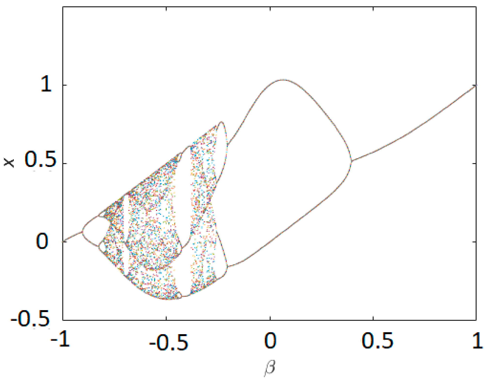
2.1. One Dimensional Gauss Map

Carl F. Gauss [18] invented the Gauss or Gaussian map, which is a non-linear iterated function of accurate intervals with real parameters as $\alpha$ and $\beta$ that is expressed mathematically, as shown in (1):

$$y_{n+1}=e^{-\alpha \times y_n\times y_n}+\beta$$

(1)

Here real space in the characteristics can be chaotic. The map is also known as the mouse map because its bifurcation diagram is shaped like a mouse, as shown in Figure 1.

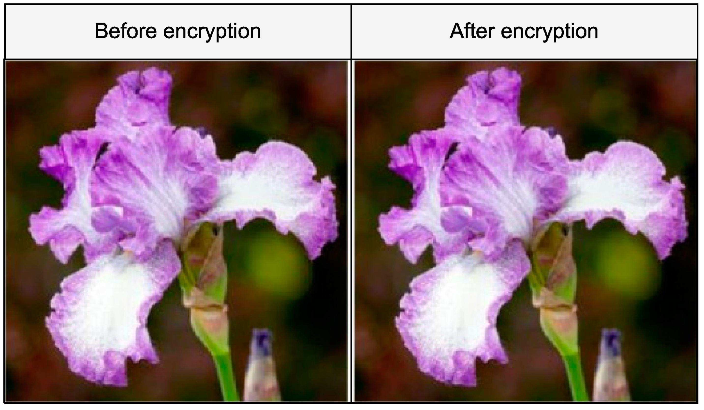
2.2. Classification of Encrypted Images

Because of the fast-growing field of artificial intelligence and data science, the proposed digital algorithms must be learning-friendly, meaning the algorithms should have good results in the machine learning environment. Therefore, the deep learning classification is demonstrated with a brief overview of the pre-trained network and transfer learning to testify to the proposed novel method.

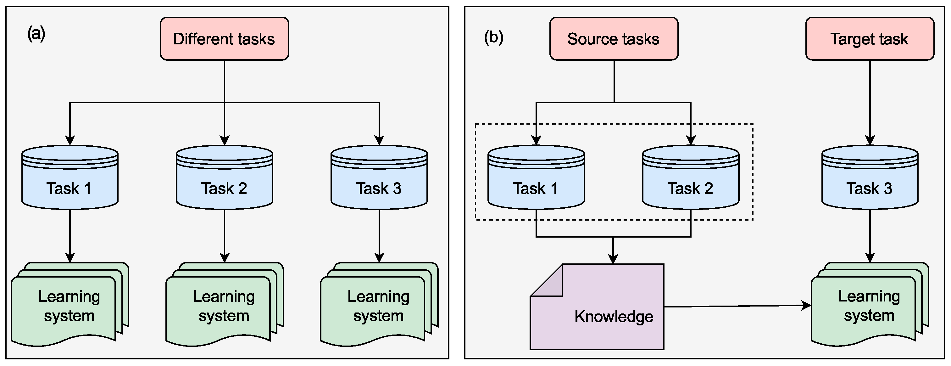
2.3. Transfer Learning vs. Machine Learning

A typical hypothesis in classical machine learning is that the training and testing data have the same feature space and data distributions, as shown in Figure 2a. When a new job arrives with a different data distribution than the prior one, a new model should be built from the ground up using the current data. Such solutions necessitate tremendous effort and thus are, in most situations, extremely expensive.

The concept of transfer learning was developed to speed up the learning process and acquire better alternatives [19]. It was influenced by the fact that human beings may intelligently use the knowledge obtained in the past when dealing with a problem they have never encountered previously [20,21]. In contrast to typical machine learning approaches, transfer learning sustains data distribution differences. It applies the knowledge collected from other sources to the target task, as shown in Figure 2b.

Deep learning implementations frequently employ transfer learning. A pre-trained network can be used as a preliminary step for learning a new task. Transfer learning is often considerably quicker and more efficient than training a network from the start with randomly initialized weights for fine-tuning [20]. With a reduced number of training images, it is possible to feed learned characteristics to a fresh, swiftly

The following are the key benefits of transfer learning over machine learning:

• It allows you to train systems with less labeled data by reusing popular models that have previously been trained on massive datasets, making transfer learning a popular approach;
• It has the potential to cut down on training time and computer resources. The weights are not learned from starting with transfer learning since the pre-trained model has previously learned them based on earlier learning;
• You can use model topologies produced by the deep learning scientific community, such as AlexNet, GoogLeNet, and ResNet, which are popular designs

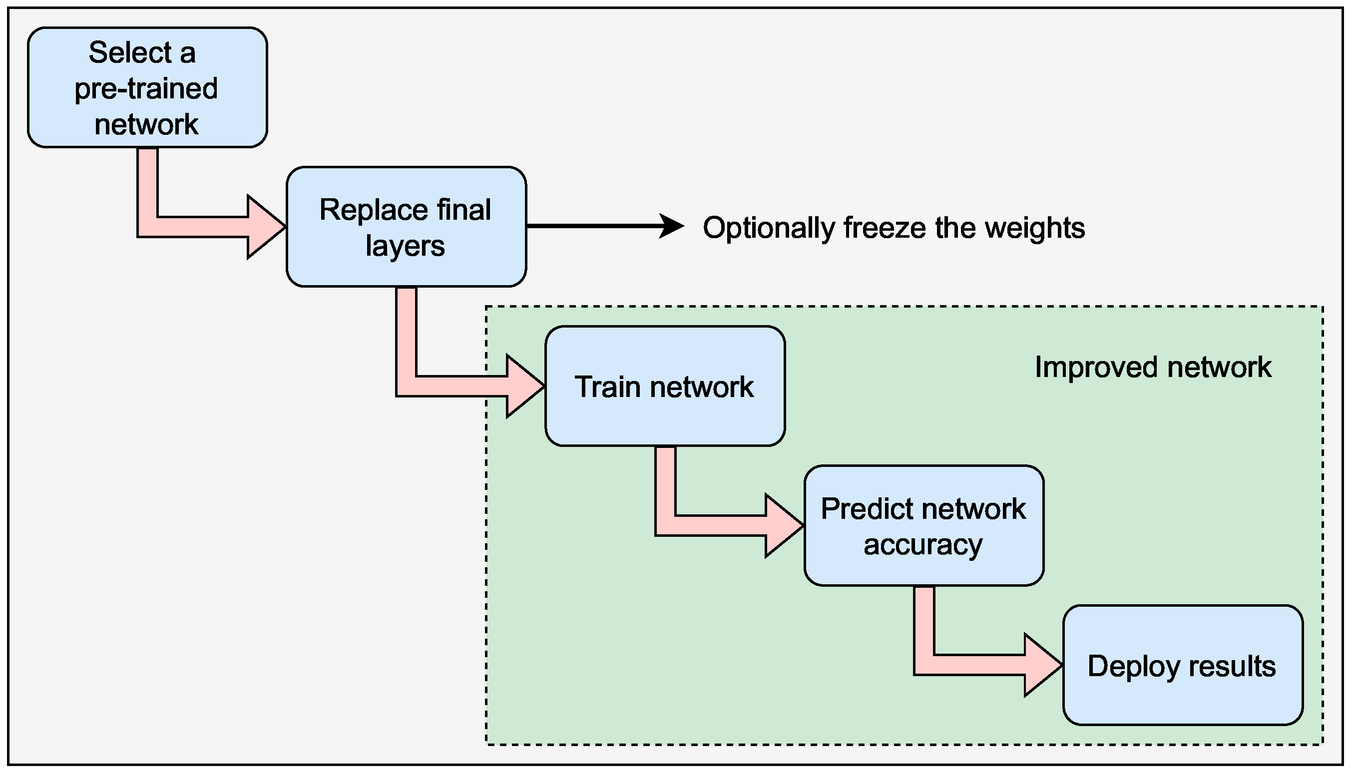
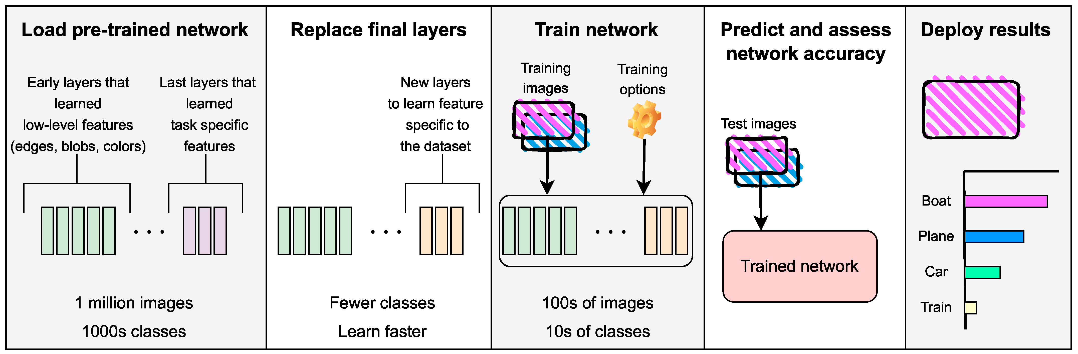
The Transfer Learning Workflow of Figure 3 is as follows:

1.

Selecting a pre-trained model: It is simpler to function with pre-trained models since there are many of them accessible on multiple platforms such as Googlenet, Squeezenet, and others;

2.

Replacement of final layers: The final layers of the chosen pre-trained model are changed to retrain the network and to categorize a fresh batch of images and classes. The final wholly linked layer is changed to get a similar number of nodes as the number of new classes and a new classification layer that will provide an output based on the probabilities estimated by the layer. The final wholly linked layer will describe the new number of network classes that will it learn after the layers have been modified. The classification layer will select outputs from the new output categories accessible after modifying the layers;

3.

Freezing the weights (Optional): By limiting the learning rates in such layers to zero, the weights of earlier layers in the network may be frozen. As a result, the characteristics of frozen layers are not modified throughout training; this significantly accelerates network training. In addition, freezing weights can help the network prevent overfitting if the new data set is tiny;

4.

Retraining the model. The network will be retrained to understand and recognize the attributes associated with the new data and categories. Retraining usually needs less data than training a model from the start;

5.

Predicting and assessing network accuracy. For example, one may classify fresh images and evaluate how well the network works once the model has been retrained [22].

Figure 3. Classification with pre-trained deep network.

Figure 3. Classification with pre-trained deep network.

2.4. Deep Network Designing with MATLAB

Deep network designer, which is available across many frameworks, may be used to develop, create, and apply pre-trained models using transfer learning for deep neural networks. For this, MATLAB Deep Network Designer is utilized in this article. With a convolutional neural network, one may do numerous classification and regression tasks on various types of data such as text, numbers, and images. It may be used in a wide variety of applications such as;

• Time Series Forecasting;
• Classification of Sequences;
• Regression from one sequence to the next;
• Classification of Text Data;
• Classification of Image Data;
• Semantic Segmentation of Multispectral Images;
• Speech Recognition;
• Image Deblocking;
• Removing noise from a Color Image Using Pretrained models, and so on.

In this article, the classification application is employed over encrypted decrypted images to testify to the suitability of the proposed encryption algorithm for the classification problem.

2.5. Transfer Learning Using AlexNet

Pretrained image classification networks, such as AlexNet, can classify pictures into 1000 item categories using the datasets provided and can be trained on over a million photographs. The networks have developed rich feature representations for a wide variety of pictures.

The network takes an image as input and generates labels for each object in the image and probabilities for each object category [23]. The network’s convolutional layers extract visual features, then employed by the final learnable and classification layer to categorize the input picture. The training process using AlexNet is shown in Figure 4.

3. Proposed Method

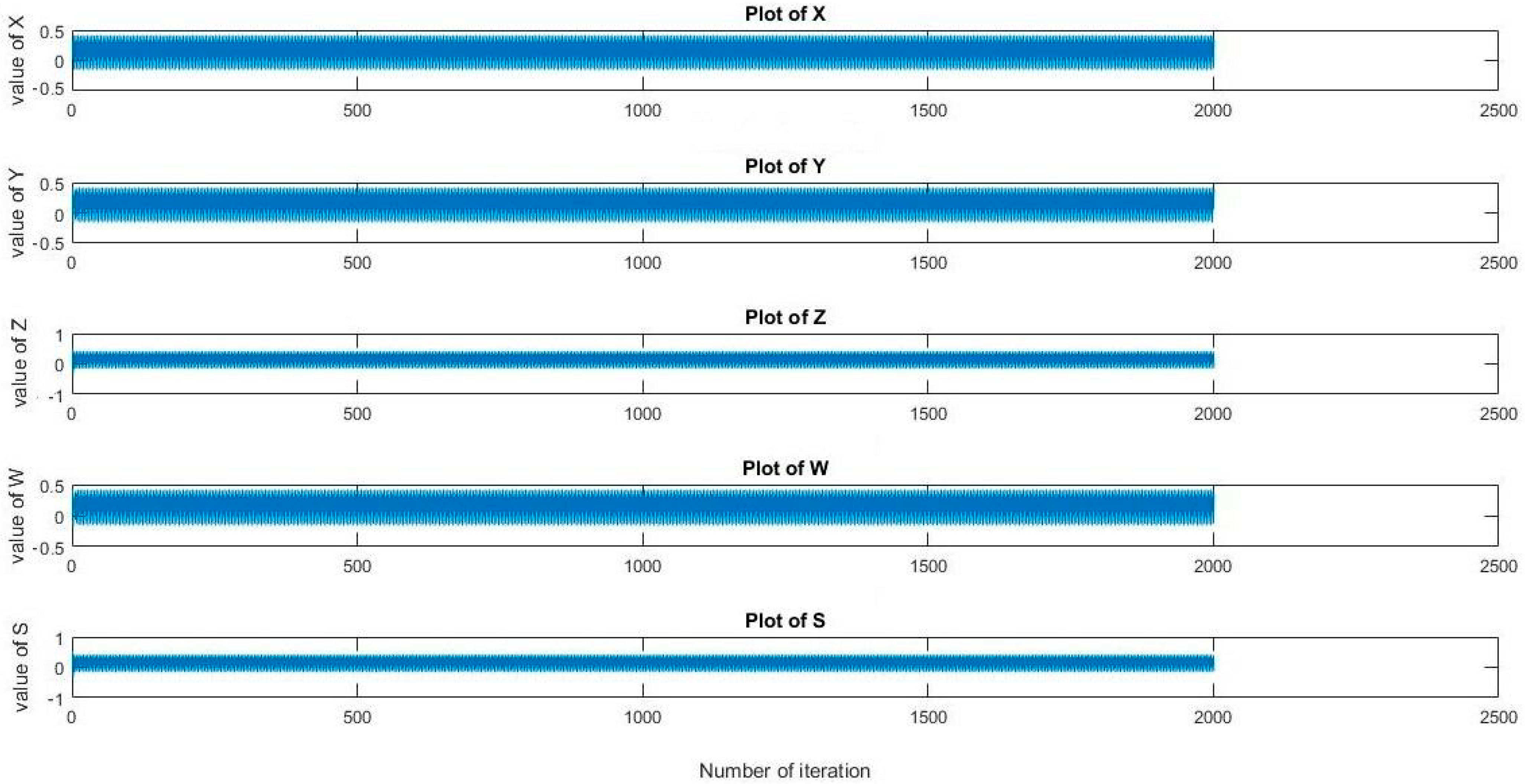
3.1. 5D Gauss Map Equation and Plot (Iteration)

A chaotic map generates pseudo random values, and is then utilized in the encryption operation. The input parameters influence the pseudo-randomness of the outcomes produced by chaotic maps. In this paper we developed the idea of the five dimensions Gauss map by using (1), which is as follows:

$$x_{i+1}=e^{(-c{x}_i^2)}+d+b{y}_i^2{x}_i+a{z}_i^3$$

(2)

$$y_{i+1}=e^{(-c{y}_i^2)}+d+b{z}_i^2{y}_i+a{x}_i^3$$

(3)

$$z_{i+1}=e^{(-c{z}_i^2)}+d+b{x}_i^2{z}_i+a{y}_i^2$$

(4)

$$w_{i+1}=e^{(-c{w}_i^2)}+d+b{s}_i^2{w}_i+a{z}_i^2$$

(5)

$$s_{i+1}=e^{(-c{s}_i^2)}+d+b{x}_i^2{s}_i+a{w}_i^2$$

(6)

Here, x, y, z, w, and s are intervals, and a, b, c, and d are real parameters. 5D Gauss map is more complicated and secure because of quadric, cubic, quadratic coupling, and four constant terms. Plotting of x, y, z, w, and s components are shown in Figure 5. These plots describe the value range of x, y, z, w, and s. Plots horizontal axis shows a number of iterations, and the vertical axis shows the components range.

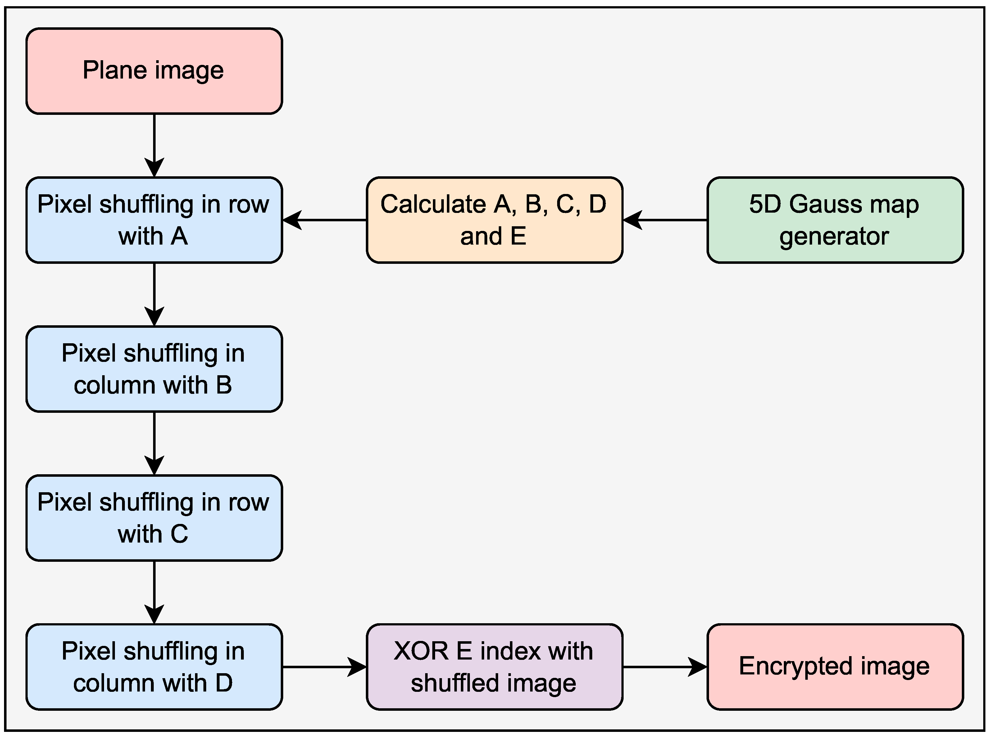
3.2. Algorithm for Image Encryption

3.2.1. 5D Gauss Generator

The Generator creates a 5D Gauss Map throughout this procedure. By the virtue of Equations (2)–(6), and starting values of $x_1=0.3250$, $y_1=0.4250$, $z_1=0.5250$, $w_1=0.4350$, $s_1=0.5350$, $a=0.0135$, $b=0.0177$, $c=4.9$, and $d=-0.58$, it creates chaotic sequences. Any value between zero and one for the initial values of the variables can be chosen here.

3.2.2. Permutation

• Random numbers are selected to achieve pixel permutation, P, Q, and R;
• With the help of these numbers, five sequences or indexes A, B, C, D, and E are generated;
• A pixel is shuffled in a row with sequence A and in a column with sequence B to create confusion;
• Here two times shuffling is done with row and column, the first time with A, B sequence and the second time with C and D sequence;
• The XOR process is the final stage in this encryption procedure. When using the XOR technique, the pixel intensities are changed to a new one, which cannot be inverted unless having the chaos key.

The flow diagram in Figure 6 expresses the above-stated encryption algorithm, which is detailed in the following steps:

• Step 1: Read plaintext image I (the image size is set to $256\times 256$ pixels);
• Step 2: The chaotic sequences are constructed iteratively using the Gauss chaotic Equations (2)–(6) and the initial values of x, y, z, w, and s;
• Step 3: Using random numbers and chaotic sequences, generate index sequences A, B, C, D, and E;
• Step 4: To produce a confusion matrix, bring the index sequence A from Step 1 and shuffle the pixels in rows and columns with sequence B;
• Step 5: Pixels are shuffled in the row with sequence C and in the column with sequence D once more, resulting in scrambled image $IS$;
• Step 6: The index sequence E is then XORed with the scrambled image $IS$, resulting in the encrypted image.

Figure 6. Flow diagram of the encryption process with a 5D Gauss map.

Figure 6. Flow diagram of the encryption process with a 5D Gauss map.

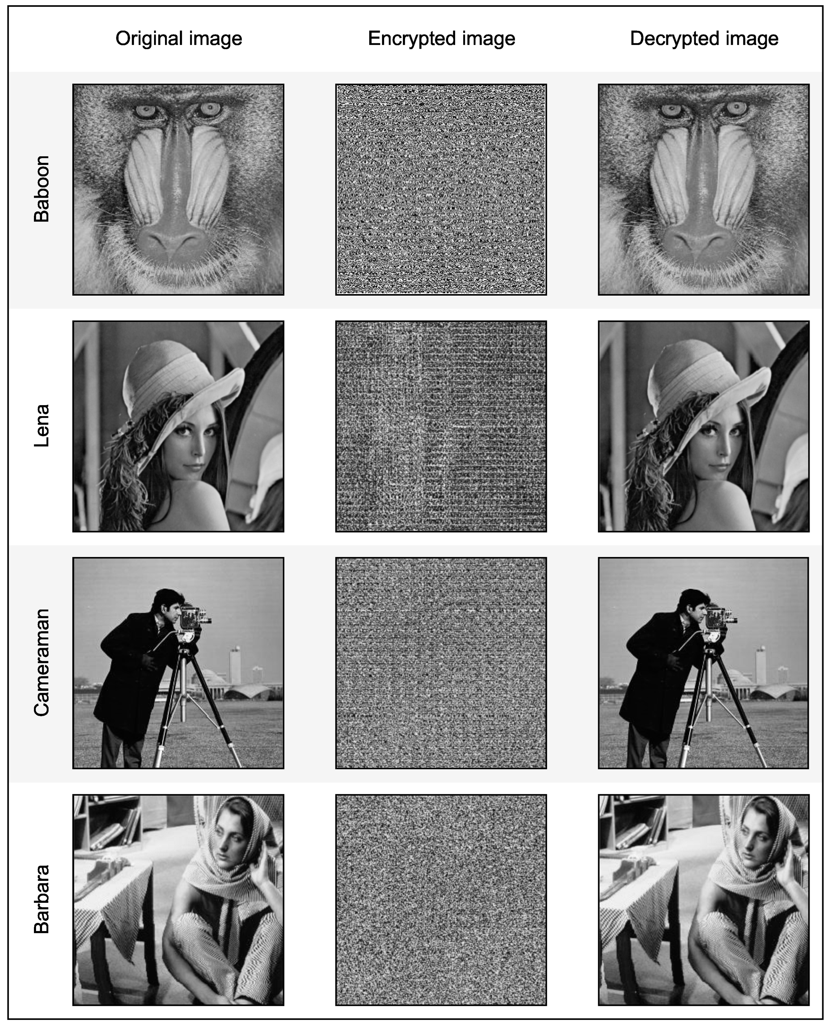
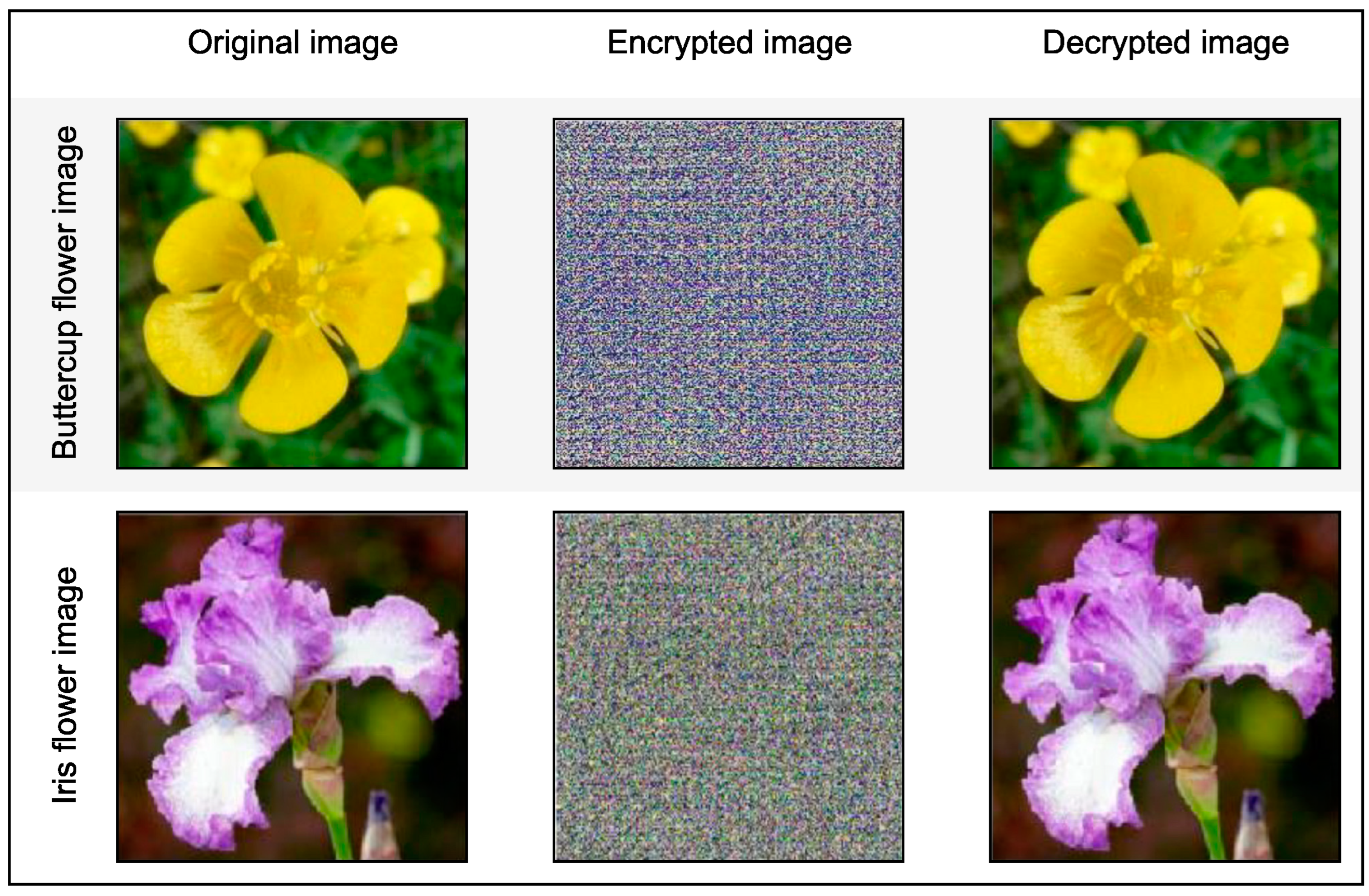
4. Results and Facts

The simulations are performed in the Matlab environment to evaluate the algorithm’s effectiveness and validate it. Figure 7 and Figure 8 illustrate the original, encrypted, and decrypted $256\times 256$ test images and histograms, respectively.

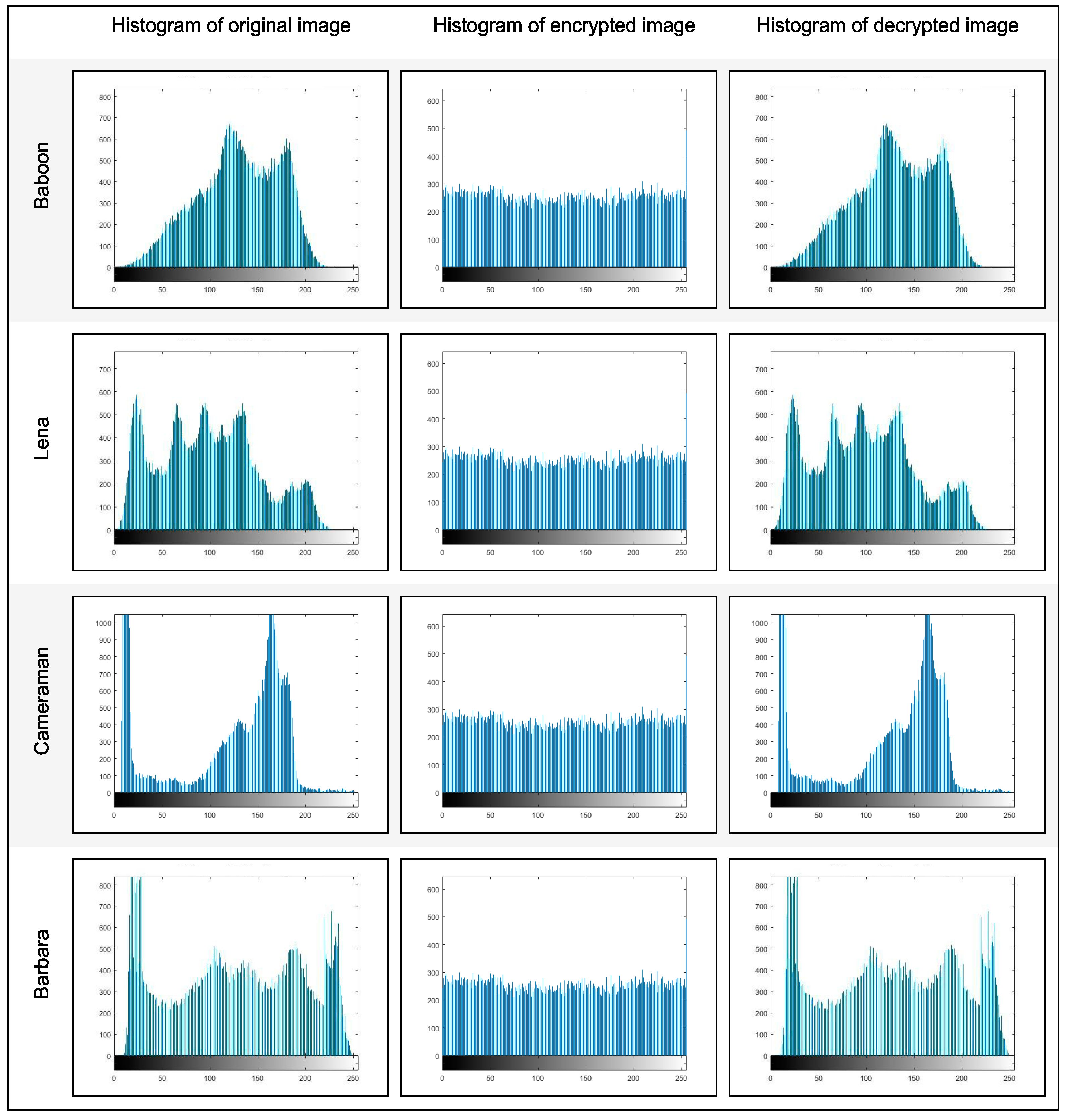
4.1. Information Entropy

Information entropy serves as an indicator and technique of unpredictability in information theory. The quantity of entropy can always be utilized to characterize the outcome of plaintext and ciphertext confidentiality. The greater information entropy shows better security. For example, a value of 8 for the information entropy of the cipher image suggests that pictures are exceptionally near to random distribution, and the security is more remarkable [24]. Mathematically it is expressed as shown in (7).

$$IE=\sum _{i=1}^{n}P(Y=y_i)\log P(Y=y_i)$$

(7)

where Y is a discrete random variable with values $\{y_1,y_2,\cdots ,y_n\}$, and i is an integer variable with values ranging from 1 to n.

In the equation, $P(Y=y_i)$ is the probability of Y taking the value of $y_i$, this denotes the fraction of all Y occurrences with the value $y_i$.

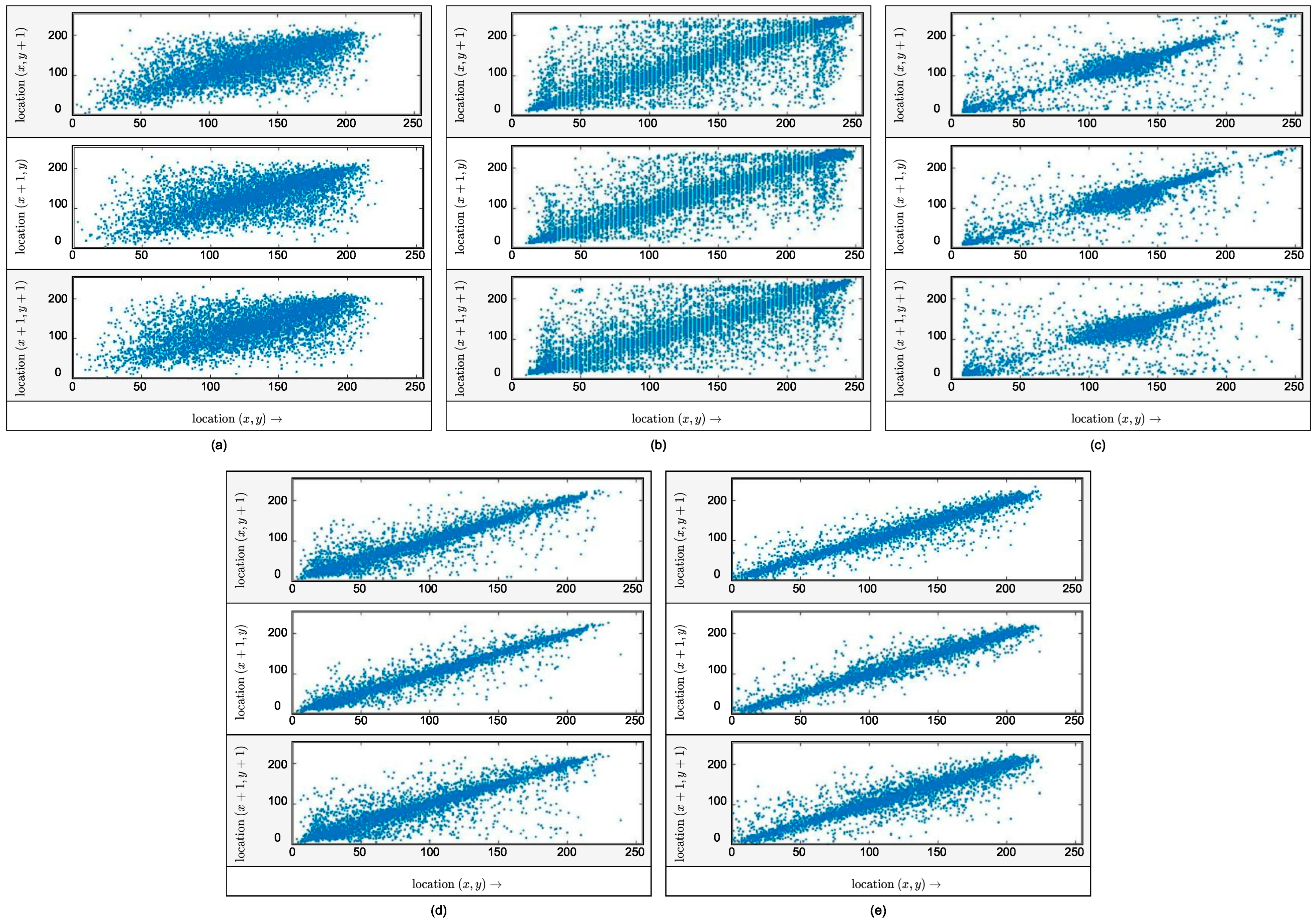
4.2. Correlation Coefficient (CC)

The horizontal, vertical, and diagonal correlation between the two input images before and after encryption can be determined at various levels. The correlation coefficients (CC) are shown in Figure 9 and Figure 10, implying that there is essentially no relationship between the two. This shows that the key in this article is sensitive to the parameters and the security of the encryption scheme [25].

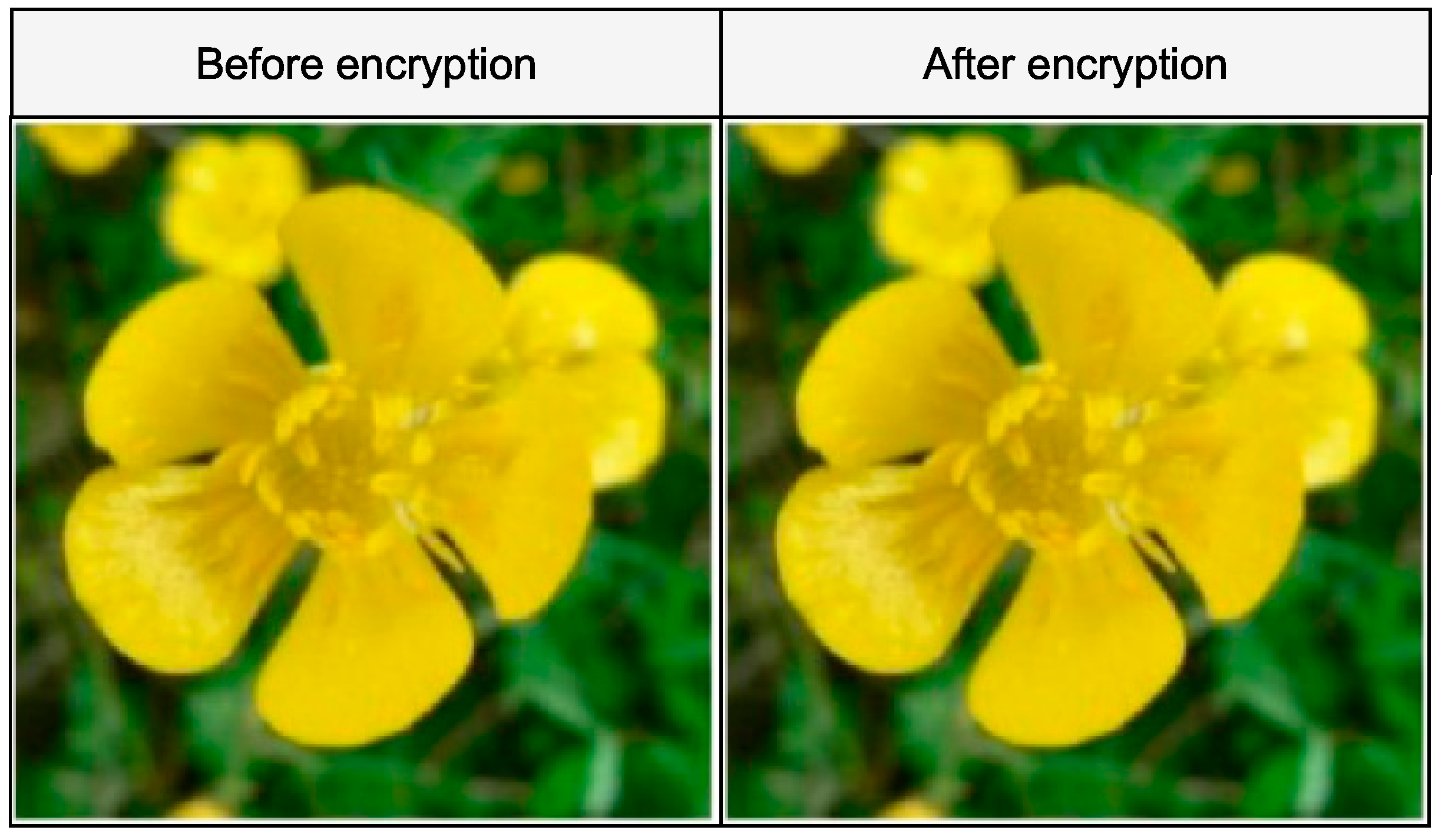
4.3. PSNR, MSE, and SSIM

PSNR and SSIM should be higher for encryption reliability, but MSE must be lower. The equation of the $PSNR$, $MSE$, and $SSIM$ are represented as (8)–(10), respectively.

$$PSNR=10{\log }_{10}\left[\frac{256\times 256}{MSE}\right]$$

(8)

$$MSE=\frac{1}{MN}\sum _{i=0}^{M-1}\sum _{j=0}^{N-1}{[f^{\prime }(i,j)-f(i,j)]}^2$$

(9)

$$SSIM(f,g)=l(f,g)c(f,g)s(f,g)\left\{\begin{array}{c}l(f,g)=\frac{2{\mu }_f{\mu }_g+C_1}{{\mu }_f^2+{\mu }_g^2+C_1}\\ c(f,g)=\frac{2{\sigma }_f{\sigma }_g+C_2}{{\sigma }_f^2+{\sigma }_g^2+C_2}\\ s(f,g)=\frac{{\sigma }_{fg}+C_3}{{\sigma }_f{\sigma }_g+C_3}\end{array}\right.$$

(10)

4.4. Differential Attack

A differential attack is a method of attacking an encryption scheme by comparing and analyzing specific variations in plaintext in relation to changes conveyed during encryption.

The ability to withstand differential attacks is tightly linked to the plaintext image’s sensitivity. Computing the encoded image’s pixel change rate ($NPCR$) and the unified average change intensity ($UACI$) may also be used to assess the method’s capacity to withstand differential attacks. NPCR and UACI analysis are the most frequent methods for determining plaintext sensitivity. The NPCR and UACI mathematical structures are stated as shown in (11) and (12).

$$NCPR=\frac{1}{M\times N}\sum _{i=1}^M\sum _{j=1}^{N}K(i,j)\times 100\%$$

(11)

$$UACI=\frac{1}{M\times N}\sum _{i=1}^M\sum _{j=1}^N\frac{|a_1(i,j)-a_2(i,j)|}{255}\times 100\%$$

(12)

Table 1. PSNR, SSIM, MSE, and Entropy values for the input test images.

Images	PSNR	SSIM	MSE	Entropy Plain Image	Entropy Encrypted Image
Lena	∞	1	0	7.5694	7.9621
Man	∞	1	0	7.0097	7.8529
Peppers	∞	1	0	7.5487	7.9533
Barbara	∞	1	0	7.3410	7.9043
Baboon	∞	1	0	7.3705	7.9578
Boat	∞	1	0	7.1894	7.8794

displays distinct test scores such as, peak signal to noise ratio, mean square error, similarity index, and entropy.

Table 2. NPCR and UACI test results for different test images.

Images	NPCR (%)	UACI (%)
Lena	99.62	33.42
Man	99.59	33.35
Peppers	99.58	33.34
Barbara	99.57	33.33
Baboon	99.61	33.41
Boat	99.64	33.43

shows NPCR, and UACI results for the input test images, and

Table 3. Correlation Coefficient (CC) Horizontal (H), Vertical (V), and Diagonal (D) values for the input test images.

Images	Original			Encrypted
	CC (H)	CC (V)	CC (D)	CC (H)	CC (V)	CC (D)
Lena	0.9502	0.9712	0.9282	0.1100	−0.0664	−0.0752
Man	0.9416	0.9630	0.9136	0.0843	−0.0591	−0.0682
Peppers	0.9682	0.9725	0.9425	0.0007	0.0155	−0.0042
Barbara	0.8262	0.8942	0.8501	0.0061	−0.0159	−0.0123
Baboon	0.6940	0.6039	0.6027	0.0391	0.0131	−0.0080
Boat	0.8864	0.9204	0.8400	0.1569	−0.1549	−0.1117

depicts correlation coefficients. Finally, comparisons with other works of literature are shown in

Table 4. Correlation Coefficient and entropy comparison with state-of-the-art methods.

Images	Horizontal	Vertical	Diagonal	Entropy
Proposed	0.1100	−0.0664	−0.0752	7.9621
[26]	−0.0414	−0.0342	0.1083	7.4077
[27]	0.0039	0.0059	−0.0050	7.9994
[28]	0.0008	0.0004	0.0020	7.9995

.

4.5. Keyspace

Typically, the keyspace of an image cryptosystem should be large enough to make the brute-force search attacks difficult. Following is a formula for calculating the size of the keyspace.

Before that, it is necessary to determine which parameters were utilized as the key. The keyspace of this approach is theoretically unlimited. However, when the actual value is taken, the accuracy will be reduced due to the limitations of computational performance and precision in practical applications. Multiple cryptographic keys in the proposed system are as follows: a, b, c, d, $x_1$, $y_1$, $z_1$, $w_1$, and $s_1$. It is helpful to quantify the entire keyspace using the IEEE floating-point norm [29].

$$\mathrm{Keyspace}={10}^{15}\times {10}^{15}\times {10}^{15}\times {10}^{15}\times {10}^{15}\times {10}^{15}\times {10}^{15}\times {10}^{15}\times {10}^{15}={10}^{135}\approx 2^{448}$$

(13)

From the preceding equation, it is clear that the keyspace of the system is large enough to withstand a crypto attack.

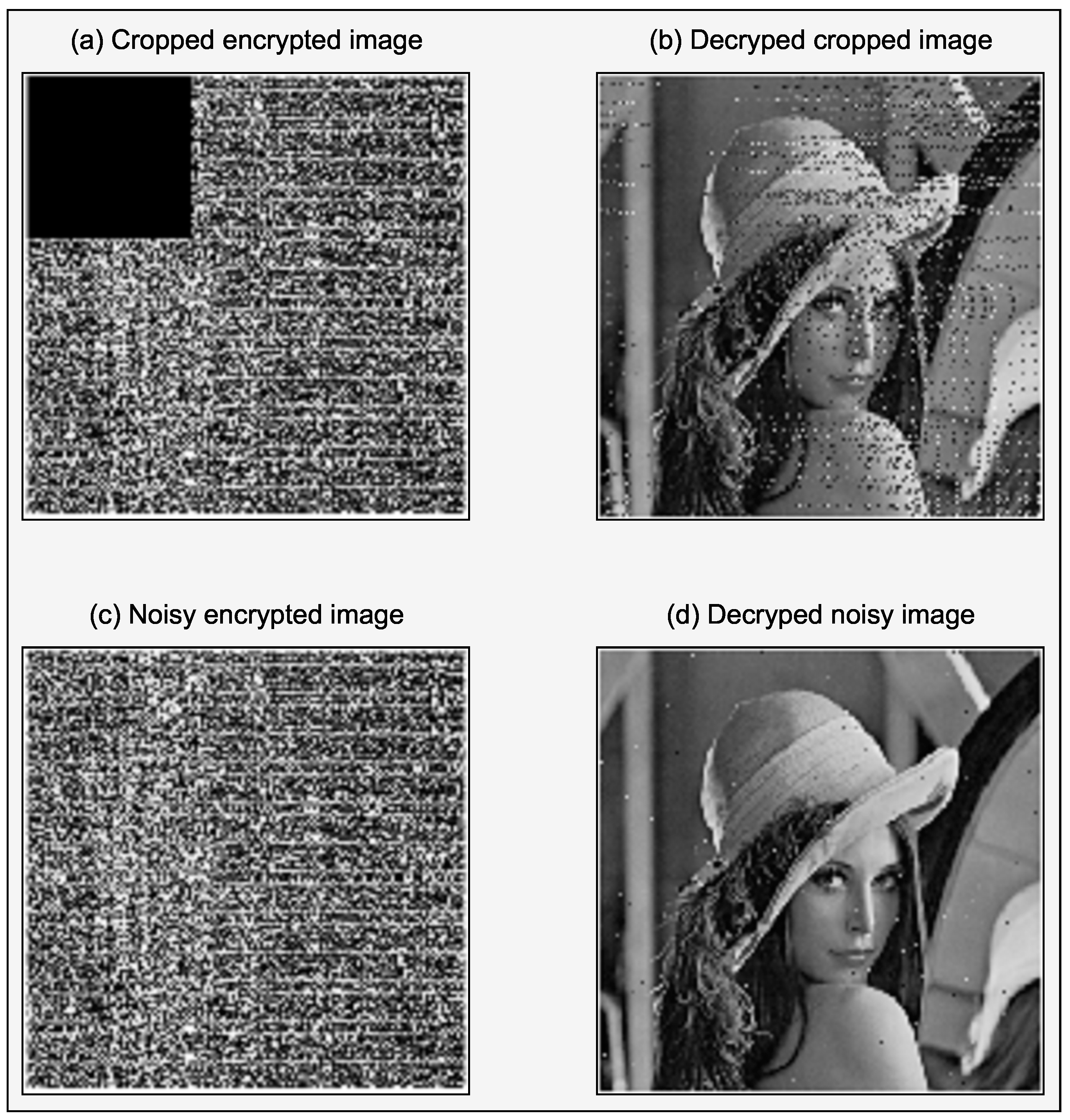
4.6. Noise and Cropping Attack

The cipher pictures can be corrupted by noise and cropping attacks when transmitted over the Internet or any other transmission method, making it impossible to extract the plain images. As a result, the performance of the proposed algorithm must be evaluated against various assaults to determine its effectiveness.

Accordingly, Lena’s $256\times 256$ pixel cipher picture has been changed by adding Cropping (data loss 6.25%) and Salt-Pepper noise (noise density 0.005), respectively, as illustrated in Figure 11. However, because of the slight PSNR variation reported in

Table 5. PSNR values of the cropped encrypted images.

Images	PSNR of the Cropped Encrypted Image	PSNR of the Noisy Encrypted Image
Lena	16.707916	32.354713
Man	17.296258	31.669253
Peppers	17.900450	32.064819
Barbara	16.708817	31.032769
Baboon	18.526831	32.952549
Boat	18.855763	33.389143

, the results suggest that the assaults had little impact on the image and visual quality of the image.

4.7. NIST Test

The National Institute of Standards and Technology (NIST) test is the most widely used method for determining if a time series is random. In the NIST test, we investigate the unpredictability of the chaotic sequences created by the Gauss map using 12 random test techniques.

Table 6. NIST test results for the 5D Guass Map.

Test	Values	Results
Frequency	0.8315	Pass
Block Frequency	0.2888	Pass
Cumulative Sums Forward	0.5120	Pass
Cumulative Sums Reverse	1.0000	Pass
Runs	0.6572	Pass
Longest Run	0.1339	Pass
Rank	0.1885	Pass
FFT	0.6250	Pass
Overlapping Template	0.3525	Pass
Approximate Entropy	0.9875	Pass
Linear Complexity	0.1045	Pass
Serial	0.1514	Pass

shows the NIST test results for the proposed method.

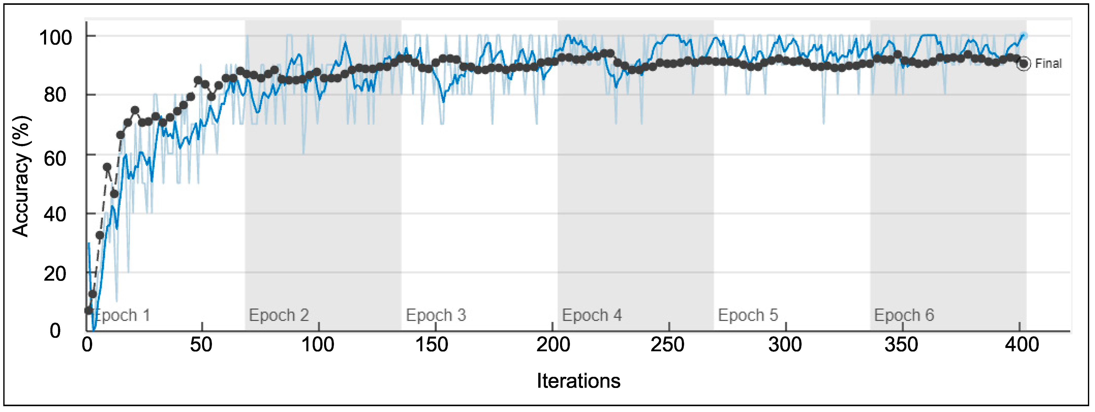
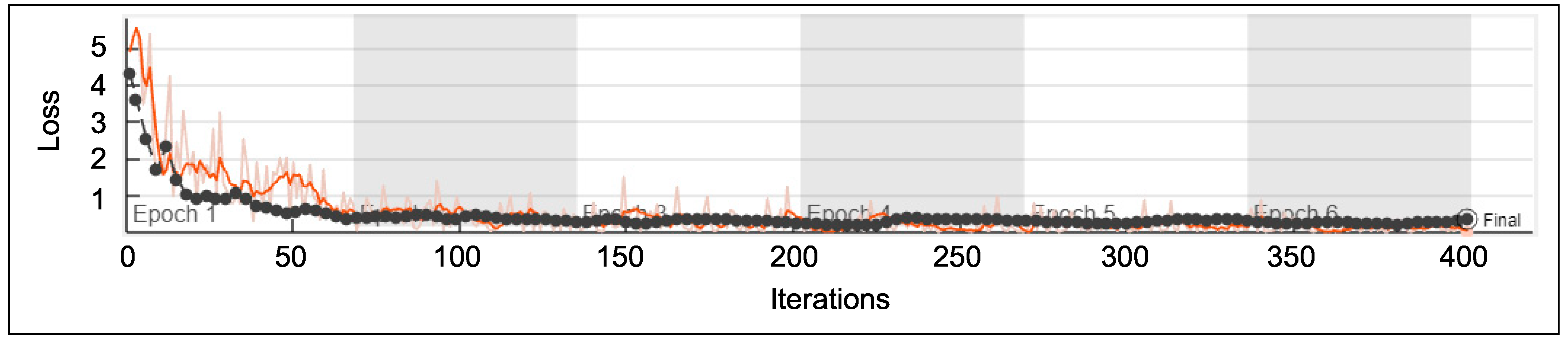
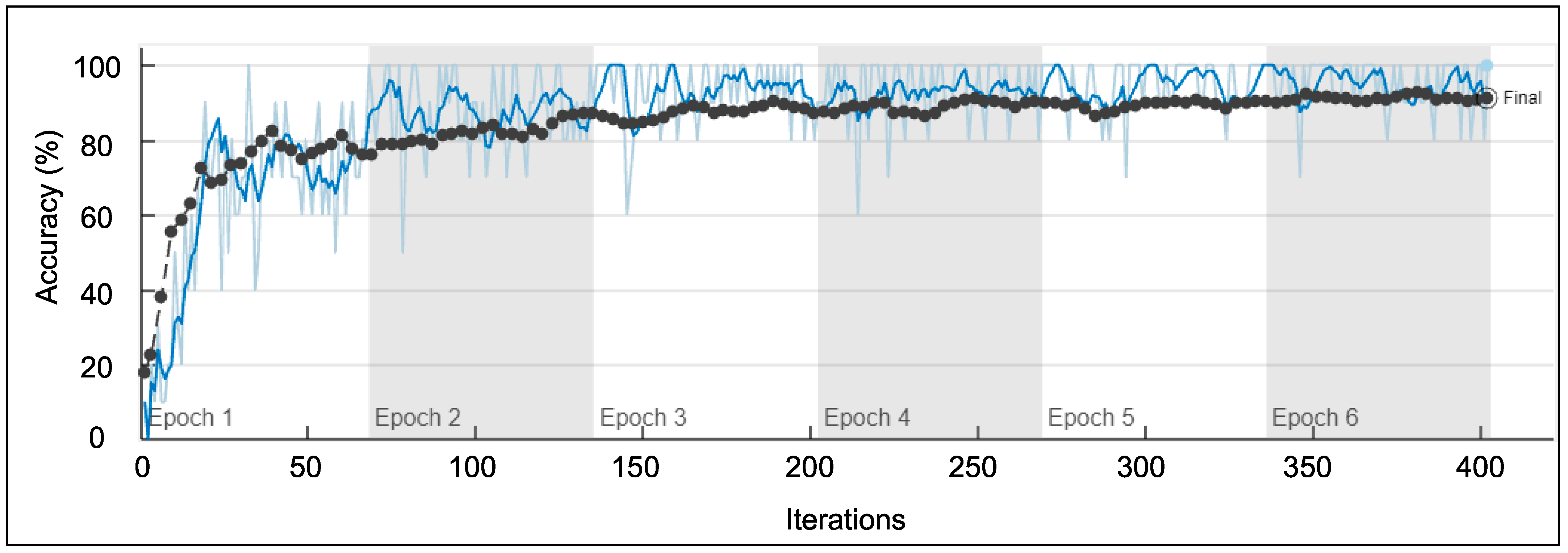
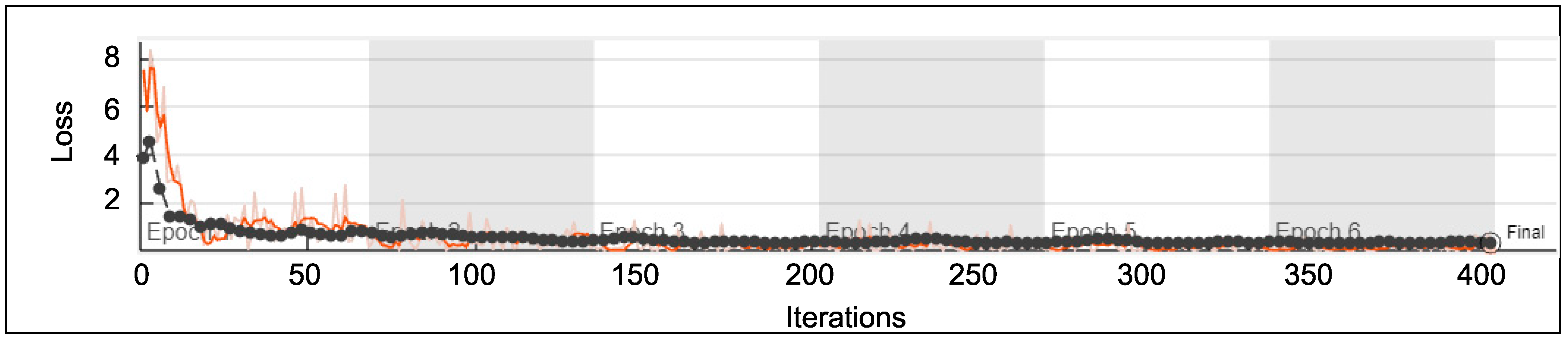
5. Validation of Classification Accuracy

In this section, the classification accuracy of the proposed encryption algorithm is tested through deep learning classification using transfer learning. Figure 12 shows the Original, Encrypted, and Decrypted buttercup and iris images, which are further used to test the classification accuracy. The AlexNet transfer learning model on the deep learning designer of MATLAB 2021 is used here for the simulation. Figure 13 shows the classification of buttercup images before and after encryption. Furthermore, it is advent from the results that the images encrypted through the proposed method were classified accurately.

Figure 14 and Figure 15 show the accuracy versus iteration graph, and the loss versus iteration graph for the buttercup image, respectively.

Figure 16 shows the classification of iris images before and after encryption. Furthermore, it is advent from the results that the images encrypted through the proposed method were classified accurately.

Figure 17 shows the accuracy versus iteration graph, and Figure 18 shows the loss versus iteration graph for the iris image. The validation accuracy of buttercup and iris image is 90.62% and 91.35%, respectively.

It is advent from the results of this section that the method not only works well with color images but also has decent classification accuracy too.

6. Conclusions

This article presented a modified 5D version of an existing 1D Gauss map for image encryption. The method’s significant benefit is essential, nonlinear, but has a high-dimensional structure, which is simple to build but highly complex in real behavior due to the increased number of parameters and extensive shuffling operation of rows and columns. The PSNR value and the attacks validate the proposed system’s efficacy. The algorithm performs admirably in the face of attacks. The classification accuracy of the encryption algorithm is also validated with transfer learning. Through the NIST test, it is proved that the 5D Gauss generation scheme presented can provide substantial assurances for image security and advances the new five-dimensional idea of image security research. This experiment also provides some information on how to create additional 5D chaotic maps that can be used to add high security to image and visual data. Further, the classification experimentation with transfer learning recommends that the encryption algorithm is also suitable for classification problems.

References

1. Wong, K.W.; Kwok, B.S.H.; Yuen, C.H. An efficient diffusion approach for chaos-based image encryption. Chaos Solitons Fractals 2009, 41, 2652–2663. [Google Scholar] [CrossRef] [Green Version]
2. Patro, K.A.K.; Acharya, B.; Nath, V. Secure, lossless, and noise-resistive image encryption using chaos, hyper-chaos, and DNA sequence operation. IETE Tech. Rev. 2020, 37, 223–245. [Google Scholar] [CrossRef]
3. Liu, W.; Sun, K.; Zhu, C. A fast image encryption algorithm based on chaotic map. Opt. Lasers Eng. 2016, 84, 26–36. [Google Scholar] [CrossRef]
4. Yu, C.; Li, H.; Wang, X. SVD-based image compression, encryption, and identity authentication algorithm on cloud. IET Image Process. 2019, 13, 2224–2232. [Google Scholar] [CrossRef]
5. Bisht, A.; Dua, M.; Dua, S.; Jaroli, P. A color image encryption technique based on bit-level permutation and alternate logistic maps. J. Intell. Syst. 2020, 29, 1246–1260. [Google Scholar] [CrossRef]
6. Veena, G.; Ramakrishna, M. A survey on image encryption using chaos-based techniques. Int. J. Adv. Comput. Sci. Appl. 2021, 12, 379–384. [Google Scholar]
7. Jridi, M.; Alfalou, A. Real-time and encryption efficiency improvements of simultaneous fusion, compression and encryption method based on chaotic generators. Opt. Lasers Eng. 2018, 102, 59–69. [Google Scholar] [CrossRef]
8. Faragallah, O.S.; Afifi, A.; El-Shafai, W.; El-Sayed, H.S.; Naeem, E.A.; Alzain, M.A.; Al-Amri, J.F.; Soh, B.; Abd El-Samie, F.E. Investigation of chaotic image encryption in spatial and FrFT domains for cybersecurity applications. IEEE Access 2020, 8, 42491–42503. [Google Scholar] [CrossRef]
9. Tang, Z.; Yang, Y.; Xu, S.; Yu, C.; Zhang, X. Image encryption with double spiral scans and chaotic maps. Secur. Commun. Netw. 2019, 2019, 8694678. [Google Scholar] [CrossRef] [Green Version]
10. Liang, Y.R.; Xiao, Z.Y. Image encryption algorithm based on compressive sensing and fractional DCT via polynomial interpolation. Int. J. Autom. Comput. 2020, 17, 292–304. [Google Scholar] [CrossRef]
11. Sahay, A.; Pradhan, C. Gauss iterated map based RGB image encryption approach. In Proceedings of the 2017 International Conference on Communication and Signal Processing (ICCSP), Chennai, India, 6–8 April 2017; pp. 0015–0018. [Google Scholar]
12. Al-Abaidy, S.A.F. Optimal Use Of ANN In The Integration Between Digital Image Processing And Encryption Technique. Turk. J. Comput. Math. Educ. (TURCOMAT) 2021, 12, 950–958. [Google Scholar] [CrossRef]
13. Hajjaji, M.A.; Dridi, M.; Mtibaa, A. A medical image crypto-compression algorithm based on neural network and PWLCM. Multimed. Tools Appl. 2019, 78, 14379–14396. [Google Scholar] [CrossRef]
14. Hu, F.; Wang, J.; Xu, X.; Pu, C.; Peng, T. Batch image encryption using generated deep features based on stacked autoencoder network. Math. Probl. Eng. 2017, 2017, 3675459. [Google Scholar] [CrossRef]
15. Man, Z.; Li, J.; Di, X.; Sheng, Y.; Liu, Z. Double image encryption algorithm based on neural network and chaos. Chaos Solitons Fractals 2021, 152, 111318. [Google Scholar] [CrossRef]
16. Rahmawati, W.; Liantoni, F. Image Compression and Encryption Using DCT and Gaussian Map. IOP Conf. Ser. Mater. Sci. Eng. 2019, 462, 012035. [Google Scholar] [CrossRef] [Green Version]
17. Li, P.; Xu, J.; Mou, J.; Yang, F. Fractional-order 4D hyperchaotic memristive system and application in color image encryption. EURASIP J. Image Video Process. 2019, 2019, 22. [Google Scholar] [CrossRef]
18. Al-Khasawneh, M.A.; Uddin, I.; Shah, S.A.A.; Khasawneh, A.M.; Abualigah, L.; Mahmoud, M. An improved chaotic image encryption algorithm using Hadoop-based MapReduce framework for massive remote sensed images in parallel IoT applications. Clust. Comput. 2021, 25, 999–1013. [Google Scholar] [CrossRef]
19. Hashmi, M.F.; Katiyar, S.; Keskar, A.G.; Bokde, N.D.; Geem, Z.W. Efficient pneumonia detection in chest xray images using deep transfer learning. Diagnostics 2020, 10, 417. [Google Scholar] [CrossRef]
20. Zhuang, F.; Qi, Z.; Duan, K.; Xi, D.; Zhu, Y.; Zhu, H.; Xiong, H.; He, Q. A comprehensive survey on transfer learning. Proc. IEEE 2020, 109, 43–76. [Google Scholar] [CrossRef]
21. Pan, S.J.; Yang, Q. A survey on transfer learning. IEEE Trans. Knowl. Data Eng. 2009, 22, 1345–1359. [Google Scholar] [CrossRef]
22. Maniyath, S.R.; Thanikaiselvan, V. An efficient image encryption using deep neural network and chaotic map. Microprocess. Microsyst. 2020, 77, 103134. [Google Scholar] [CrossRef]
23. Hosny, K.M.; Kassem, M.A.; Fouad, M.M. Classification of skin lesions into seven classes using transfer learning with AlexNet. J. Digit. Imaging 2020, 33, 1325–1334. [Google Scholar] [CrossRef] [PubMed]
24. Pan, H.; Lei, Y.; Jian, C. Research on digital image encryption algorithm based on double logistic chaotic map. EURASIP J. Image Video Process. 2018, 2018, 142. [Google Scholar] [CrossRef]
25. Thoms, G.R.; Muresan, R.; Al-Dweik, A. Chaotic encryption algorithm with key controlled neural networks for intelligent transportation systems. IEEE Access 2019, 7, 158697–158709. [Google Scholar] [CrossRef]
26. Ferdush, J.; Begum, M.; Uddin, M.S. Chaotic lightweight cryptosystem for image encryption. Adv. Multimed. 2021, 2021, 5527295. [Google Scholar] [CrossRef]
27. Talhaoui, M.Z.; Wang, X.; Midoun, M.A. Fast image encryption algorithm with high security level using the Bülban chaotic map. J. Real-Time Image Process. 2021, 18, 85–98. [Google Scholar] [CrossRef]
28. Mondal, B.; Behera, P.K.; Gangopadhyay, S. A secure image encryption scheme based on a novel 2D sine–cosine cross-chaotic (SC3) map. J. Real-Time Image Process. 2021, 18, 1–18. [Google Scholar] [CrossRef]
29. Ahuja, B.; Doriya, R. A novel hybrid compressive encryption cryptosystem based on block quarter compression via DCT and fractional Fourier transform with chaos. Int. J. Inf. Technol. 2021, 13, 1837–1846. [Google Scholar] [CrossRef]
Figure 1. Bifurcation diagram of Gauss map.
Applsci 12 05321 g001
Figure 2. Typical (a) Machine Learning and (b) Transfer Learning processes.
Applsci 12 05321 g002
Figure 4. Transfer Learning using AlexNet.
Applsci 12 05321 g004
Figure 5. Individual plot for x, y, z, w, and s dimensions.
Applsci 12 05321 g005
Figure 7. Results of encrypted and decrypted test images.
Applsci 12 05321 g007
Figure 8. Histogram of encrypted and decrypted test images.
Applsci 12 05321 g008
Figure 9. Correlation coefficients of original images, (a) Barbara, (b) Baboon, (c) Cameraman, (d) Pepper, and (e) Lena.
Applsci 12 05321 g009
Figure 10. Correlation coefficients (H, V, and D components) of all encrypted test images.
Applsci 12 05321 g010
Figure 11. Results of encrypted and decrypted Lena image with cropping and noise attack.
Applsci 12 05321 g011
Figure 12. Original, encrypted, and decrypted Buttercup and Iris Images.
Applsci 12 05321 g012
Figure 13. Classification of Buttercup image before and after encryption.
Applsci 12 05321 g013
Figure 14. Accuracy versus iteration graph for buttercup image.
Applsci 12 05321 g014
Figure 15. Loss versus iteration graph for Buttercup image.
Applsci 12 05321 g015
Figure 16. Classification of Iris image before and after encryption.
Applsci 12 05321 g016
Figure 17. Accuracy versus iteration graph for Iris image.
Applsci 12 05321 g017
Figure 18. Loss versus iteration graph for Iris image.
Applsci 12 05321 g018