Article

Experimental Assessment of Feature Extraction Techniques Applied to the Identification of Properties of Common Objects, Using a Radar System

by
José Francisco Díez-Pastor
,
Pedro Latorre-Carmona
*,
José Luis Garrido-Labrador
,
José Miguel Ramírez-Sanz
and
Juan J. Rodríguez
Depto. de Ingeniería Informática, Universidad de Burgos, Avda. Cantabria s/n, 09006 Burgos, Spain
*
Author to whom correspondence should be addressed.
Appl. Sci. 2021, 11(15), 6745; https://doi.org/10.3390/app11156745
Submission received: 9 June 2021 / Revised: 13 July 2021 / Accepted: 21 July 2021 / Published: 22 July 2021
(This article belongs to the Special Issue Advances in Applied Signal and Image Processing Technology)

Abstract

:
Radar technology has evolved considerably in the last few decades. There are many areas where radar systems are applied, including air traffic control in airports, ocean surveillance, and research systems, to cite a few. Other types of sensors have recently appeared, which allow tracking sub-millimeter motion with high speed and accuracy rates. These millimeter-wave radars are giving rise to myriad new applications, from the recognition of the material close objects are made, to the recognition of hand gestures. They have also been recently used to identify how a person interacts with digital devices through the physical environment (Tangible User Interfaces, TUIs). In this case, the radar is used to detect the orientation, movement, or distance from the objects to the user’s hands or the digital device. This paper presents a thoughtful comparative analysis of different feature extraction techniques and classification strategies applied on a series of datasets that cover problems such as the identification of materials, element counting, or determining the orientation and distance of objects to the sensor. The results outperform previous works using these datasets, especially when the accuracy was lowest, showing the benefits feature extraction techniques have on classification performance.

1. Introduction

Radar sensing has been classically used in an extensive range of applications, due to its ability to operate under all-weather and scene illumination geometry independence acquisition conditions. This would be a critical advantage, under specific circumstances, when compared, for instance, to optical sensing. Advances in radar hardware and software technology have made it possible to reliably detect and track objects, under competitive classification accuracy conditions, in underwater, air, and ground environments [1,2]. However, this framework seems to have been applied only to relatively big objects in specific scenarios, i.e., airplanes, ships, or submarines [3,4].
Radar technology has also found an important field of application in remote sensing data classification and health monitoring for environmental preservation purposes, usually combined in a common optical remote sensing framework [5,6].
Apart from these research fields, radar sensors are also being applied nowadays in other areas, as in action and gesture recognition or in autonomous driving, to cite a few cases. In particular, there is an increasing interest in the use of radar technology in human gesture and action recognition because it is aimed at solving the problem of low recognition accuracy that vision based systems may have. Not only gestures [7] but also more complex actions are aimed at by the new radar acquisition technology and classification strategies [8]. Even daily or ordinary activities (e.g., cooking, eating, and resting) may be classified using this type of acquisition technology [9]. Usually, human action recognition is made using sensors whose location is fixed, but new approaches using unmanned aerial vehicles (UAVs) are starting to appear [10].
Another area where radar technology is being applied is related to object and people classification for systems aimed at helping create a safer driving environment, or even in autonomous driving [11,12].
Some of the newest radar sensing applications do not try to obtain information from objects over long, mid, or short distances (in the range of meters), but just within a few centimeters. A sensor developed by Google, called Soli, was announced in 2015 and obtained great media interest. It is a millimeter-wave radar, and it has found several research applications. In [13], this sensor is used to identify up to 26 types of materials and 10 body parts from several participants. In [14], it is used to classify and distinguish five common types of materials, namely aluminum, ceramic, plastic, wood, and water, regardless of their different sizes and thicknesses. A hand gesture recognition system, which successfully distinguishes 10 gestures, is proposed in [15]. This type of radar sensor has even been used for face verification [16] or to differentiate between blood samples of disparate glucose concentrations in the range of 0.5 to 3.5 mg/mL [17]. However, the number of research studies focused on the application of this technology for daily object material classification and other interactions seems to still be scarce [18]. A Tangible User Interface (TUI) allows the user to interact with digital information through real actions. This type of user interfaces is known to be more usable and easier to understand, especially for elderly people [19], since, although not everyone knows how to operate a keyboard or mouse, everyone is familiar with grasping or moving common objects. The idea behind TUIs is that there is a direct link between the digital system and the way the physical objects are manipulated.
Miniature milimeter-wave radar sensing has been proposed to enhance the interactions by identifying materials or estimating the orientation or distance at which the physical elements are located [18]. Millimeter-wave radar technology could be considered a cost effective option for material identification, counting objects/items, or estimating their position, even when they might be partially covered or occluded. This property is a great advantage when compared to other sensors such as cameras.
The aim of this paper is to apply a diverse group of classification strategies and feature extraction techniques on a series of datasets of different nature, acquired by a portable radar sensor, aiming at validating this technology as a good candidate to be used in TUI sensing problems. The classification strategies include Random Forests [20] and Support Vector Machines [21]. Moreover, different classifiers are combined in ensembles, using Stacked Generalization [22].
The feature extraction techniques applied in this paper are the basic aggregation features (e.g., averages and root mean squares) previously used by Yeo et al. [18] and two techniques originally introduced for time series classification: ROCKET [23] and TSFRESH [24]. The datasets used in this study, obtained using a radar system, are not time series. Nevertheless, as in time series, the features are arranged and therefore their order is important. For instance, functions on the values in an interval (e.g., the first half of the series or channel) can be used. Hence, methods proposed for times series classification can also be used for this kind of data. It is common practice to use time series classification methods (including multivariate time series) for datasets where the feature order is important even though the features do not represent different times [25,26], for instance, from spectroscopy [27,28]. Image contours or outlines, such as arrowheads [29], leaves [30], or fish species [31], can be represented as time series.
The rest of the paper is organized as follows. Section 2 describes the group of datasets, as well as the corresponding feature extraction and classification algorithms used. Section 3 discusses the results. These results are validated and analyzed using average rankings and post hoc tests such as the Nemenyi test, as well as by using Bayesian Signed-Rank Test, all of them in order to determine which combination of feature vector and classification method is best, and whether this improvement (i.e., difference in accuracy performance) is statistically significant or not. Section 4 presents the conclusions and discusses potential future lines of research.

2. Datasets, Feature Extraction, and Classification Methods

Radar sensing uses an electromagnetic signal that hits an object. This signal might be directly reflected or scattered/absorbed by it, therefore giving an overview of the properties of the material the object is made of or of the distance or position the object is at. The type of radar whose data form the repository we used is a Frequency-Modulated Continuous-Wave (FMCW) radar, and this type of radar system has shown its potential to be used for detection/recognition purposes.
Soli [18] is a mono-static, multi-channel (8 channels = 2 transmitters × 4 receivers) radar device, operating in the 57–64 GHz range (center frequency of 60 GHz), using an FMCW principle, where the radar transmits and receives information on a continuous basis. When an object is placed on the top or nearby the Soli sensor, the energy transmitted from the sensor is absorbed and scattered by the object, which varies depending on its distance, thickness, shape, density, internal composition, and surface properties, commonly described as the Radar Cross Section (RCS). As a result, the signals that are reflected back represent rich information about the contributions from a range of surface and internal properties.
Nevertheless, the complex mixing nature of the signals obtained by the radar sensor (due to these above-mentioned multiple factors that are contributing to the final, detected, and signal) make them have non-smooth and complex shapes, which contribute with an additional complexity degree to a potential signal classification strategy.
The aim of Section 2 is to present a coherent explanation of the different feature extraction techniques and classification strategies applied on a series of datasets obtained by Yeo et al. [18], using the Soli radar sensor. It is composed of the following subsections: Section 2.1 gives a detailed overview about the different types of datasets used in our classification performance analysis framework. Section 2.2 explains the feature extraction methods that are applied. Feature selection methods are considered taking into account their number in relation to the number of instances of each dataset (the so-called curse of dimensionality). Section 2.3 describes the different classification strategies applied.

2.1. Radar Datasets

A previous study [18] showed that Soli could be used to identify materials, estimate number of objects, their orientation, or the the distance to the sensor. Yeo et al. [18] created a series of supervised classification datasets, formed by on the one hand the signal acquired by this sensor, and the class of the material on the other hand. The type of material, distance, and other features were also included. The following is a brief schematic description about the different types of categories these datasets are formed by:
Material identification (of the material an object is made of), from a limited list of materials.
Object identification, from a series of objects in the same category (i.e., a credit card of a specific bank from the rest of the credit cards).
Counting the number of elements that might be piled up on the surface of the sensor.
Distance estimation, from an object to the sensor.
Order identification, of the items in a battery of objects.
Flipping identification, where the orientation of an object may be inferred.
Movement, where the angular position of the object or changes in the movement of one of them in relation to other(s) are obtained.
The complete group of datasets can be found at: https://github.com/tcboy88/solinteractiondata (accessed on 18 January 2021). As stated above, the radar chip has eight channels that acquire a series of raw signals. Each of these channels has 64 data points. This information is converted into a 512 (= 64 × 8 ) feature vector and collectively saved in a CSV file. Therefore, the original dataset dimensionality value is always constant and equal to 512. As recommended by Yeo et al. [18], the easiest way to use the data was considering the Weka Graphical User Interface (GUI), converting them to Attribute-Relation File Format (i.e., .arff) files. This final group of datasets is formed by 34 files.
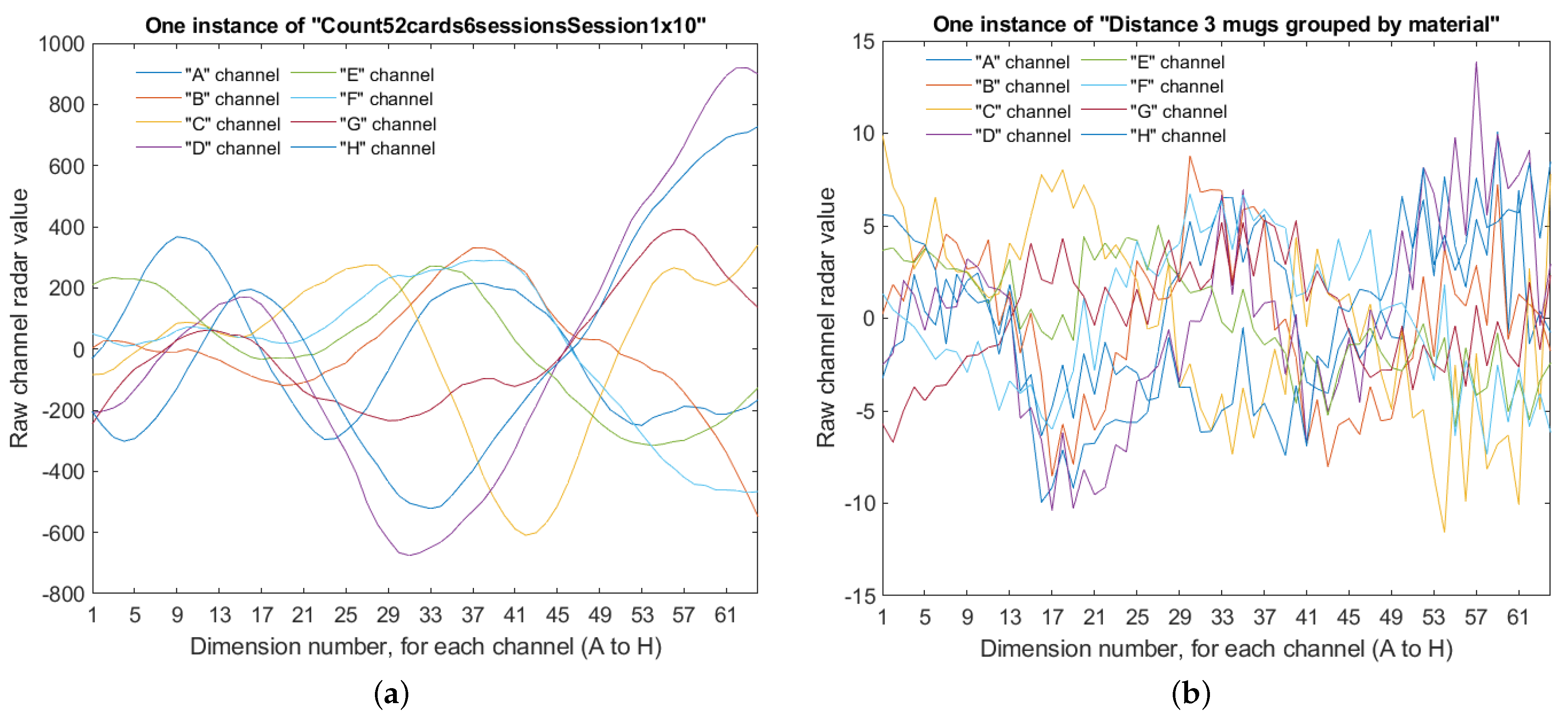
Figure 1a,b shows the eight 64D signals obtained by the radar sensor for two instances, each from a different dataset. We can see the complex and irregular shape of the signals detected by the sensor.
Table 1 shows the total number of samples and classes for each one of the files. These datasets show different acquisition conditions over a series of distinct objects, including playing cards, poker chips, and Lego blocks. For particular details and a deeper description about the acquisition conditions for the creation of these sets, the reader is referred to Section 6 in [18].

2.2. Feature Extraction

The most straightforward way to apply a classification strategy on this dataset would be to use the complete 512-dimensional vector (raw data) as the feature vector. However, raw data often contain noise, redundancies, or irrelevant information; thus, there are different feature selection/extraction techniques that could be applied on such a feature space and subsequently be used instead or added to this feature vector. The following additional feature extraction techniques are considered in our case:
  • Basic aggregation features: A series of basic features are extracted. They are defined as aggregations at different levels:
    Along the signals of the eight channels: Average (AVG) and the average of the absolute values (ABS). There are 64 values in each case and 128 (= 64 × 2 ) values in total.
    For each channel (×8): Absolute mean square (AMS) and root mean square (RMS). There are 8 for each channel and 16 values in total.
    At a global level: Maximum, minimum, mean, AVG, average of absolute values (ABS), and root means square (RMS). There are five values in total.
  • ROCKET (RandOm Convolutional KErnel Transform [23]): It is a method that achieves state-of-the-art classification accuracy in several benchmarks, but it only requires a fraction of the training time used by other existing standard methods. Other methods for time series classification focus only on a single type of representation such as shape, frequency, or signal variance. Convolutional kernels are able to represent multiple characteristics of different types simultaneously.
  • TSFRESH (Time Series FeatuRe Extraction based on Scalable Hypothesis tests): This methodology aims to avoid the time-consuming process of meaningful feature identification and extraction, from time series data. It consists of an algorithm and a Python package. The Python package implements the extraction of 794 features using multiple characterization methods, each of them executed with various sets of parameters. This framework also includes feature selection to identify those features that are statistically significant. The algorithm is described in [32]. The software package is presented in [24]. The total number of features is therefore 6352 (= 8 × 794 ).
In this framework, each feature vector is individually analyzed in relation to its significance for predicting the target class label. As a result, a vector of p-values is obtained. This vector is assessed against the Benjamini–Yekutieli procedure [33], which allows the method to decide which features to keep. This selection strategy considers the application of a threshold, whose default value is 0.05. However, this selection is so restrictive in some cases that most of the features are discarded. An iterative method is applied that considers the threshold values 0.05 , 0.1 , 0.2 , 0.5 and selects the first one that keeps at least a 10% of the total number of attributes.

2.3. Classification Methods

Two main blocks of classification strategies were considered to be applied on the datasets, summarized as the use of: (a) a Support Vector Machine and a Random Forest classifier, being these two classifiers those that were used in [18] (presented in Section 2.3.1); (b) a Stacked Generalization approach (a particular type of ensemble machine learning algorithm) (Section 2.3.2), where we try to take advantage of the diversity that different classification methods may give, in order to help improve classification accuracy, when using them in a coordinated/simultaneous way.

2.3.1. Single Type Classifiers

Two classification methodologies were applied: (1) Support Vector Machines (SVM); (2) Random Forests (RFs). SVM is a widely used classification method, in different and varied areas of research, partly because of its capability and good behavior when dealing with problems with a small number of samples in (relation to) high-dimensional feature spaces. Originally developed and applied in linearly separable problems, it is aimed at obtaining the hyperplane whose distance to the two groups of data points (called margin), representing the two classes, was maximal. SVM was generalized later to deal with nonlinearly separable problems using the so-called (transformational) Kernel trick [21]. A mathematical transformation function is applied to map the nonlinear separable dataset into a higher dimensional space where the samples can be linearly separated using an hyperplane.
Under this mathematical framework, two parameters emerge ( C , γ ) . The optimal value of these parameters is problem dependent. A Grid Search strategy was applied to assess their optimal values. The parameter C search interval and step size was 2 5 , 2 3 ,…, 2 15 , and the corresponding γ interval and step size was 2 15 , 2 13 ,…, 2 3 . Whenever the best best pair of parameters was obtained in the interval limits, the Grid Search was automatically extended by a factor of two. This procedure follows the guidelines given in [34].
Ensemble learning methods are based on the idea of using multiple learning algorithms to obtain better predictive performance than one could obtain from any of them, separately. The idea behind ensemble learning is the way an expert committee works in real life, i.e., it is usually easier to properly predict something when the prediction is made by more than one expert, and a consensus is obtained from them. Ensembles are combinations of several classifiers, which are often called base classifiers. There are several types of ensembles, which may be divided into two large groups: (a) homogeneous ensembles, where all the base classifiers are built using the same algorithm (but with different versions of the dataset or different training parameters); (b) heterogeneous ensembles, where the base classifiers are built using different algorithms.
Diversity is a key property in the search for an optimal ensemble strategy performance, since there is no benefit when combining base classifiers that always obtain the same predictions. There are several techniques to induce diversity in homogeneous ensembles. In Bagging [35], for instance, each classifier is trained with a variant of the training dataset, which uses different random samples of the training set. Random Forests [20] are ensembles of Decision Trees [36]. In this method, the diversity during the training process is enforced by combining the sampling of the training set, as Bagging does, with the random selection of subsets of attributes in each node of the tree. This way, in each node, the splits only consider the selected subset of attributes. Later, on the prediction stage, each base classifier predicts a class, and the class selected the most (the mode) is the final prediction of the ensemble. RFs are used to correct the tendency of the decision trees to overfit. The main parameter of an RF is its size (i.e., the number of trees that are generated into the ensemble). In our study, 100 decision trees were used because it is a usual and sufficient number [37].

2.3.2. Stacked Generalization

Stacked Generalization is an ensemble method where a new model learns how to best combine the predictions from multiple existing models. In this approach, any learning algorithm could be used to combine them.
In particular, the generation of classifiers that are accurate and diverse is only the first part in an ensemble classifier generation process. The second part (as important as the former one) is the method used to obtain the ensemble outputs by combining the outputs of the base classifiers. Two of the approaches used to combine the outputs of the base classifiers are: (a) majority voting; (b) average of probabilities. Alternatively, there are methods that may be able to learn the so-called combination rules. These methods (called meta-classifiers) are particularly useful when the base classifiers do not have the same success rate (among them) when classifying instances. This may happen when the base classifiers are generated using different training sets or different training algorithms.
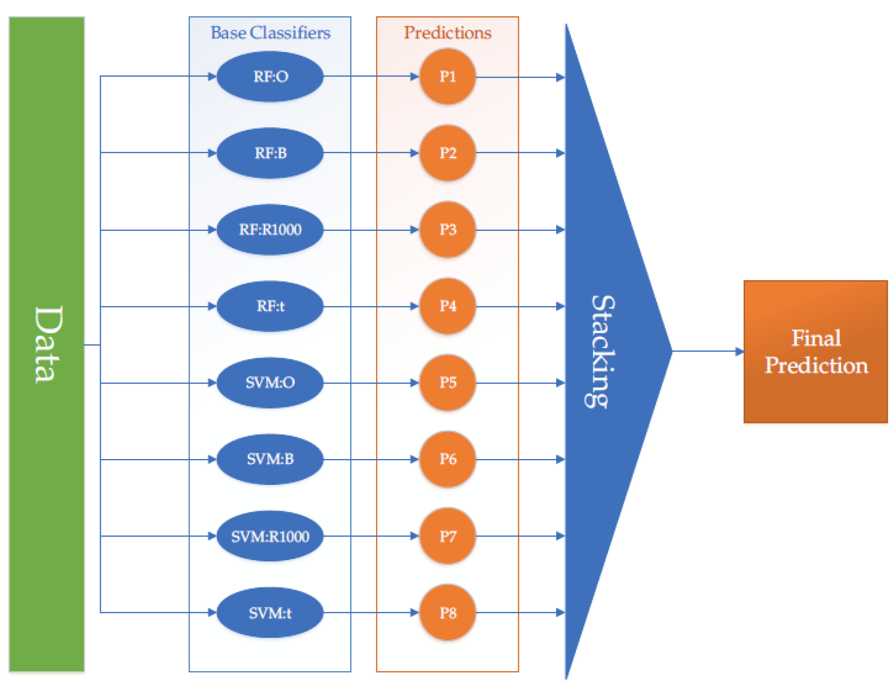
Stacked Generalization (also called Stacking) [22] builds a classifier that takes as inputs values, the output values of the base classifiers, and learns to map these values of the base classifiers into the correct final output value. In other words, no voting strategy is applied in order to combine the predictions of the base classifiers. In this case, a meta-classifier is used. The base classifiers are trained with the training set and the meta-classifier is trained with the predictions of the base classifiers. Figure 2 shows a scheme of one of the stacking approaches used.
The predictions of the classifiers are obtained from a different partition set than the one used for training. This is achieved by dividing the training set into several partitions. Therefore, Stacking can also be seen as a sophisticated form of attribute extraction. Stacking base classifiers are usually trained using different algorithms. Another strategy would be to use different views, i.e., subsets of attributes obtained by each feature extraction method. This type of Stacking strategy is often called multi-view stacking and has been successfully used when applied to other (but somehow similar) problems [38,39,40].
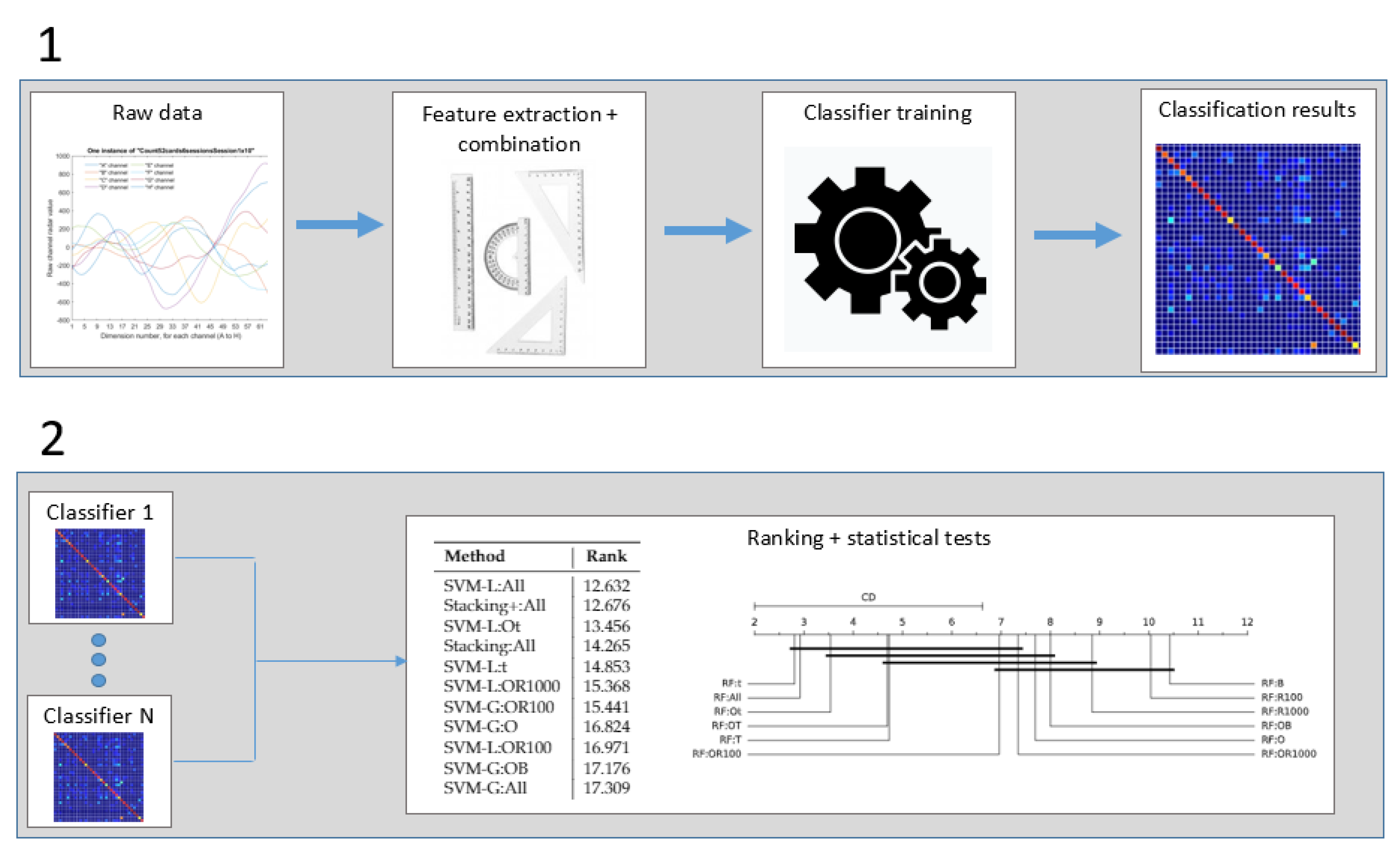
Figure 3 shows a flow diagram of the general data processing strategy followed in the paper. The figure shows the processing chain divided into two parts. The first of them shows that different types of features and feature combination strategies are obtained from the raw data values, and different classifiers are trained and used to obtain the classification accuracy results for the different datasets. In the second part, these classification accuracy results, for each dataset, are ranked, and the statistical significance of their differences are obtained in order to assess which method is better, and whether the differences among classification strategies are statistically significant or not.

3. Results and Discussion

Accuracy (for the Random Forest, SVM Linear with default parameters (rhe same configuration as the one used in [18]), and the optimized Gaussian SVM classifiers) was assessed using different combinations of the attributes explained in Section 2.2. Table 2 shows these combination strategies: The symbol `&’ means that the referred attributes are concatenated. Stacking was applied using two different configurations, called as follows:
Stacking:All: Eight base classifiers were assembled (four RF classifiers and four SVM linear classifiers), one for each one of the four extracted feature sets (raw features (O), basic aggregation features (B), ROCKET with 1000 kernels (R1000), and TSFRESH with feature selection (t)).
Stacking+:All: Ten base classifiers were assembled: the eight base classifiers described in the previous case, a linear SVM, and an RF, trained in both cases with the concatenation of all the attributes.
In all the results that follow, we use SVM-L (SVM with Linear Kernel) to refer to SVM with default parameters and SVM-G to refer to Grid search-optimized SVM with RBF Kernel. We simply use RF for the Random Forest classifier. Features used for training the classifiers use the same abbreviation as that shown in Table 2.
In order to compare the performance of the different classification methods, we might use the average accuracy of each one of the pairs (Classifier:Feature Set) evaluated throughout the 34 datasets shown in Table 1. Nevertheless, when comparing multiple methods on multiple datasets, an alternative to (and sometimes more appropriate way than) comparing average accuracies is to use average ranks [41]. Average ranks are computed in the following way: For a given dataset, the methods (in this case, a method is a pair formed by Classifier and Feature set) are sorted from best to worst. The best method receives rank = 1, the second best receives rank = 2, etc. In the case of a tie, average ranks are assigned. For instance, if two methods tie for the top rank, they both receive rank = 1.5. The average ranks across all the datasets are then computed for each method.
Post hoc tests were applied in order to identify statistically significant differences among the performance results. Some of these tests are strict in the conclusions that might be obtained from them. We found that the classification accuracy results from some of the 34 datasets are substantially high, for a considerable number of methods. Therefore, aiming at inferring the classifiers and attributes that work best with the hardest datasets (i.e., those that are more interesting), the statistical comparison of the methods was carried out twice: first using all the datasets and then using the subset formed by the difficult ones (the division between easy and difficult datasets was determined based on the performance of a baseline classifier).
Post hoc tests based on mean-ranks are commonly used, but their application has been questioned recently [42]. Hence, the results are also compared with the Bayesian Signed-Rank Test [43].

3.1. Results Corresponding to All the Datasets

Table 3 shows a selection of the results, for a subset of the pairs (Classifier:Feature Set). Given the large number of pairs, it is not possible to include all the methods in a single table (Table A1, Table A2, Table A3 and Table A4 (in the Appendix A) show the complete set of results for the RF, SVM-L, and SVM-G classifiers and the Stacking strategy, respectively, considering all the datasets). The pairs in the subset were selected so that for all data sets there was some method with the highest accuracy. In some datasets, many methods share the best accuracy, so it is not possible to include all of them in the subset. Therefore, the subset of pairs was further reduced according to the average accuracy across all the datasets. Moreover, the pairs with the feature set OB were also included because it was used by Yeo et al. [18].
Table 4 presents the average accuracy of each one of the pairs (Classifier:Feature Set) assessed throughout the 34 datasets. It also shows the average ranks computed using all the methods in the experimental setup. In terms of average accuracies, the best results obtained by Shyong Yeo et al. [18] appear in the lower third of the table; SVM-L:OB (Linear SVM trained using the concatenation of Raw and Basic features) achieves an average accuracy of 91.36%. The same classifier, when trained using all features or TSFRESH with feature selection, obtains an accuracy higher than 94.5%. In terms of average ranks, the two pairs with top ranks are SVM-L:All and Stacking+:All, with average ranks below 12.7. The average rank for SVM-L:OB is 18.13.
The best five pairs according to the average accuracy and rank (in Table 4) use the feature sets (t), (All), and (Ot). Table 5 summarizes the results in Table 4 averaging for each feature set the corresponding values of RF, SVM-L and SVM-G. According to both the average accuracies and ranks, the three best feature sets are (t), (All), and (Ot).
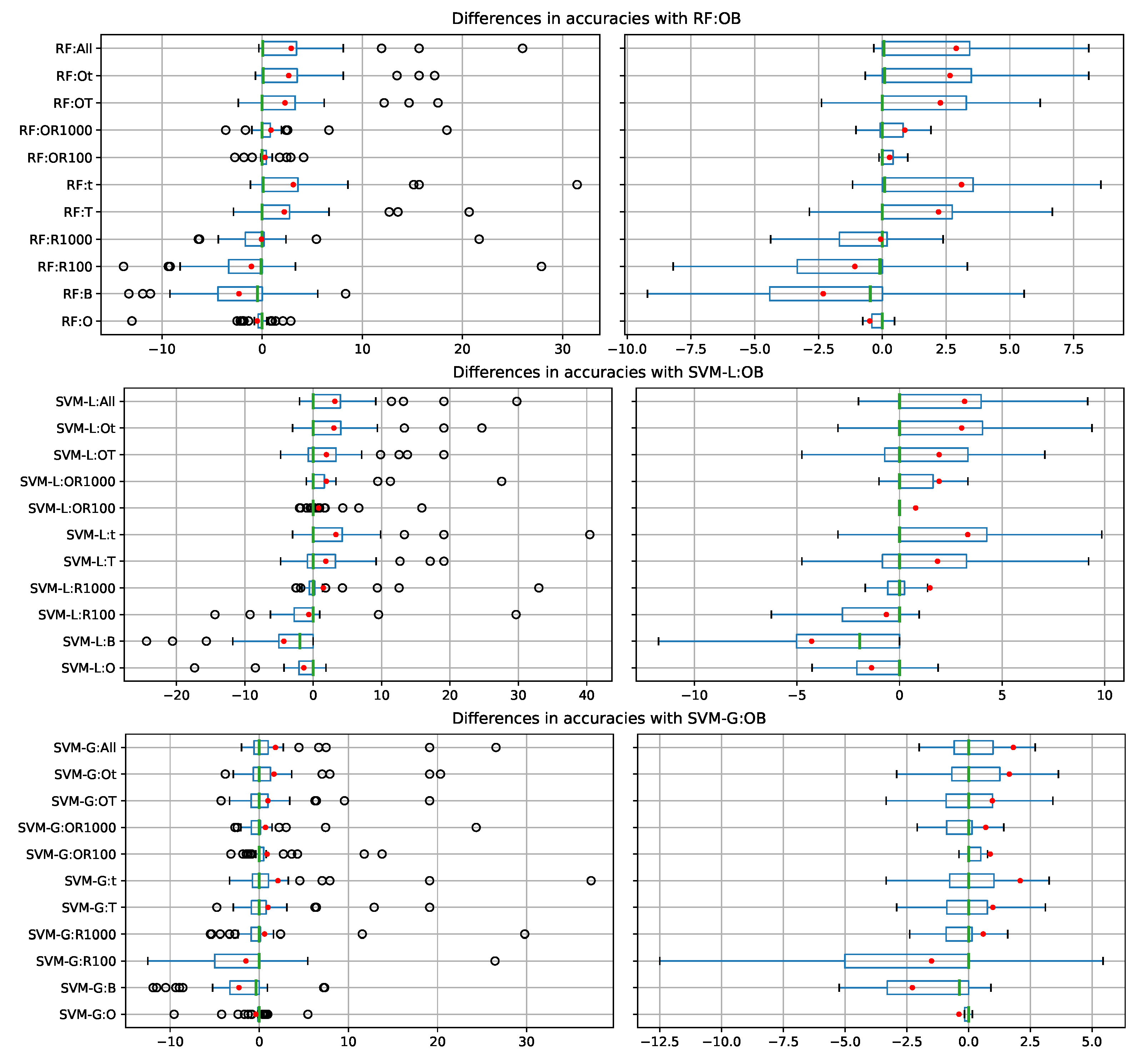
Figure 4 shows, for each one of the three classification methods, the differences in terms of accuracy between each feature set and the feature set (OB) used by Yeo et al. [18]. Each boxplot is from the corresponding differences from the 34 datasets. The average differences are clearly favorable for several of the alternative feature sets. Medians of the differences are close to 0 or negative. As shown in Table A1, Table A2, Table A3 and Table A4, there are several datasets with 100% accuracy for all or many of the feature sets. For several feature sets, the boxplot are mostly in the positive region, positive differences are greater than negative differences. For SVM-G the boxplots are less favorable to the alternative feature sets, but, as shown in Table 4, SVM-L has better results than SVM-G.
Given the large number of (Classifier:Feature Set) tested methods, it is preferable to obtain the average ranks by considering smaller pair groups. Therefore, methods were divided depending on the type of classifier used: RF, SVM-L, and SVM-G. These average ranks are shown in Table 6.
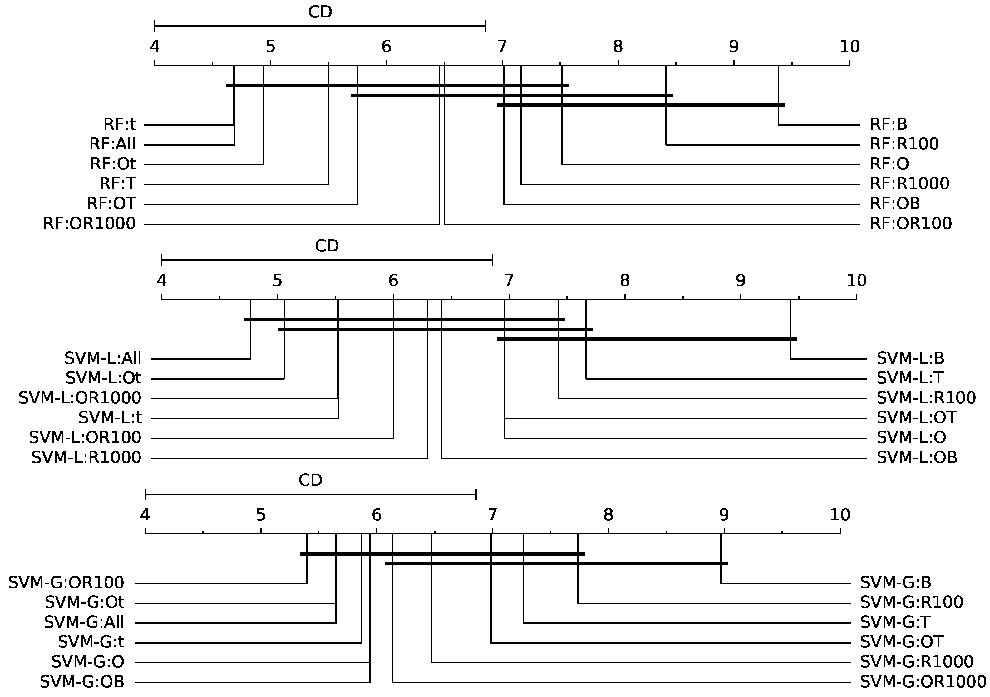
The use of the Nemenyi test [44] was also proposed by Demšar [41] to compare methods in a pairwise way. For a certain level of confidence ( α ), the test determines a critical difference (CD) value. If the difference between the average rankings of two methods is greater than CD, the null hypothesis, H 0 , that both methods have equal performance, is rejected. 
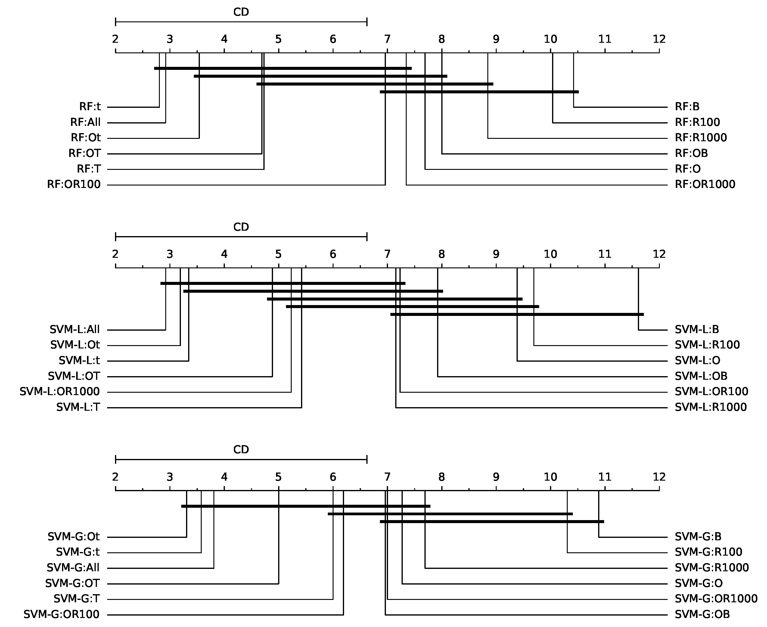
Figure 5 shows the Nemenyi’s CD diagrams. In these diagrams, thick horizontal lines are used to connect methods whose difference in average ranks is smaller than CD.
The methods were also compared using the Bayesian Signed-Rank Test [43], the Bayesian framework equivalent version of the Wilcoxon Signed-Rank Test. In this test, the value of the Region of Practical Equivalence (ROPE) was set to 1% for accuracy. Two methods were considered equivalent when the difference in their performance was smaller than this ROPE value. The test determines three probability values, corresponding to the following cases: (1) one method is better than the other; (2) vice versa; (3) they are in the ROPE.
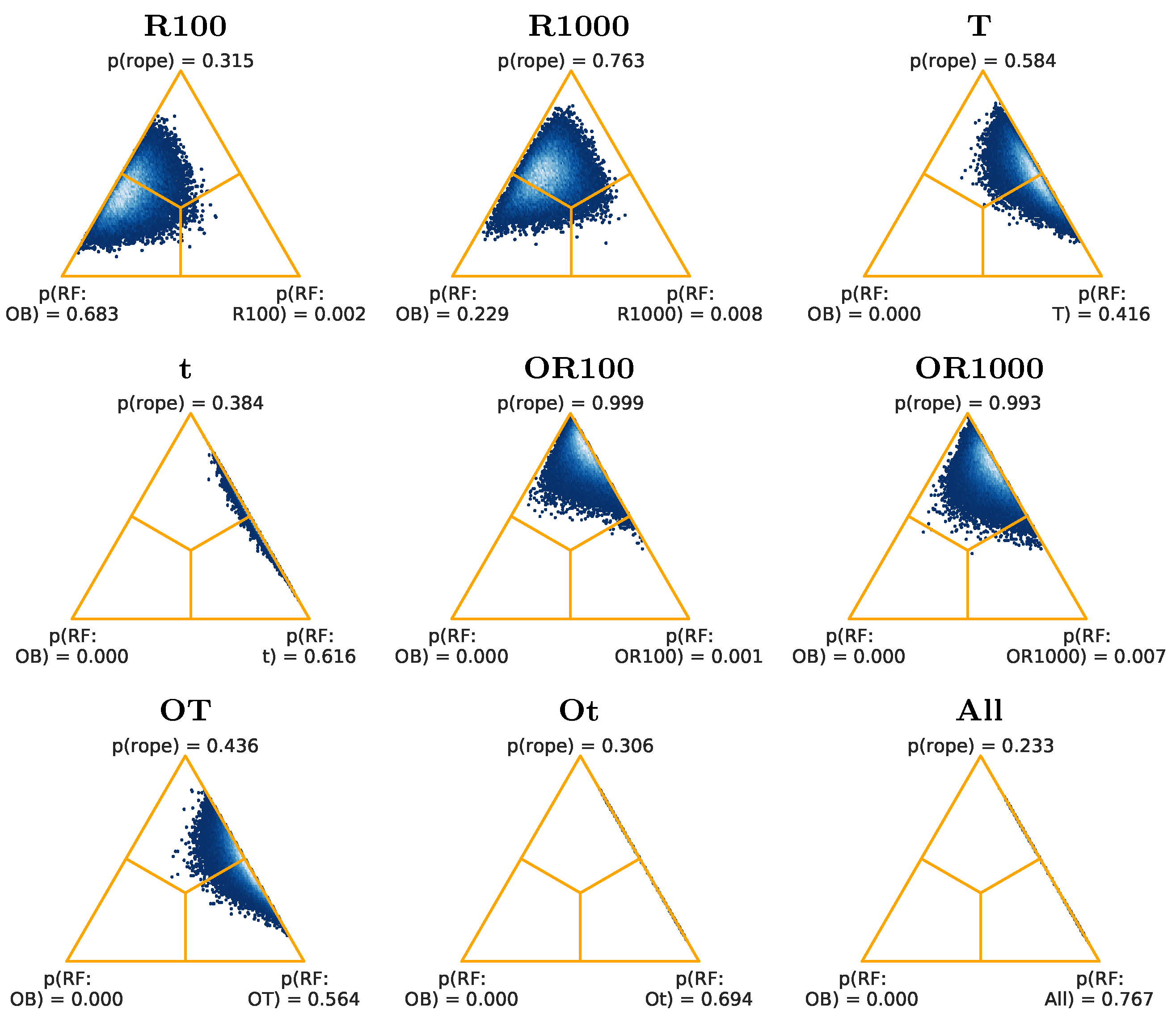
Figure 6, Figure 7 and Figure 8 show the Bayesian Signed-Rank Tests posteriors, for the RF, SVM-L, and SVM-G classifiers, respectively. In these figures, the (OB) feature set is compared against each one of the other feature sets, for the corresponding classifier. For each feature set, there is a triangle. In these triangles [43], the bottom-left and bottom-right regions correspond to the case where one method is better than the other or vice versa. The top region represents the case where the ROPE is more probable. The corner triangles show the probability of each region. The left region in the triangle is for OB and the right region for the other feature set.
Figure 6 shows that, for RF, the feature set with more favorable results when compared to (OB) is (All), with a probability of 0.767, while it is 0.000 for (OB). 
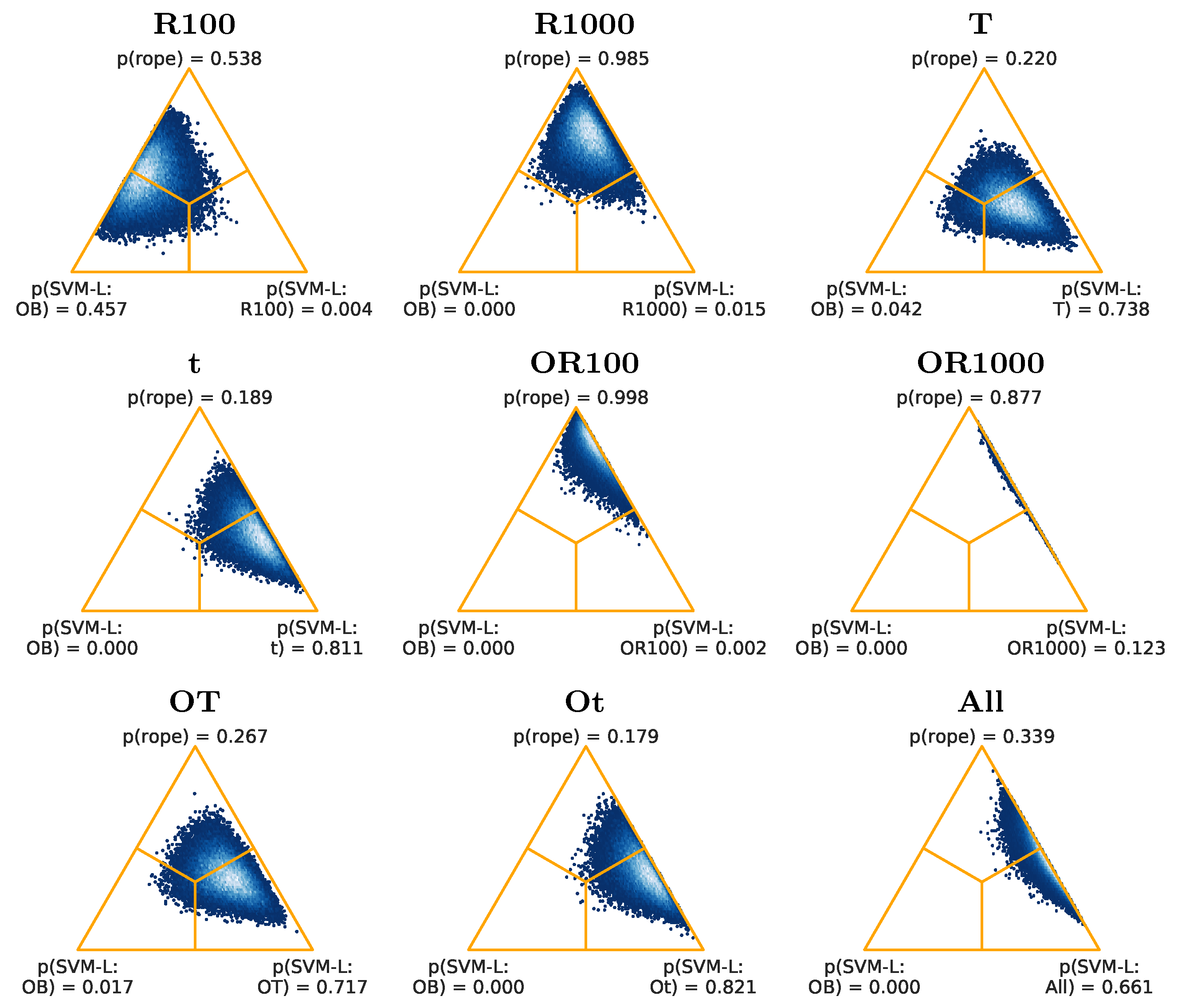
Figure 7 shows that, for SVM-L, the best feature set is (Ot): its probability is 0.821, while it is 0.000 for (OB). In 
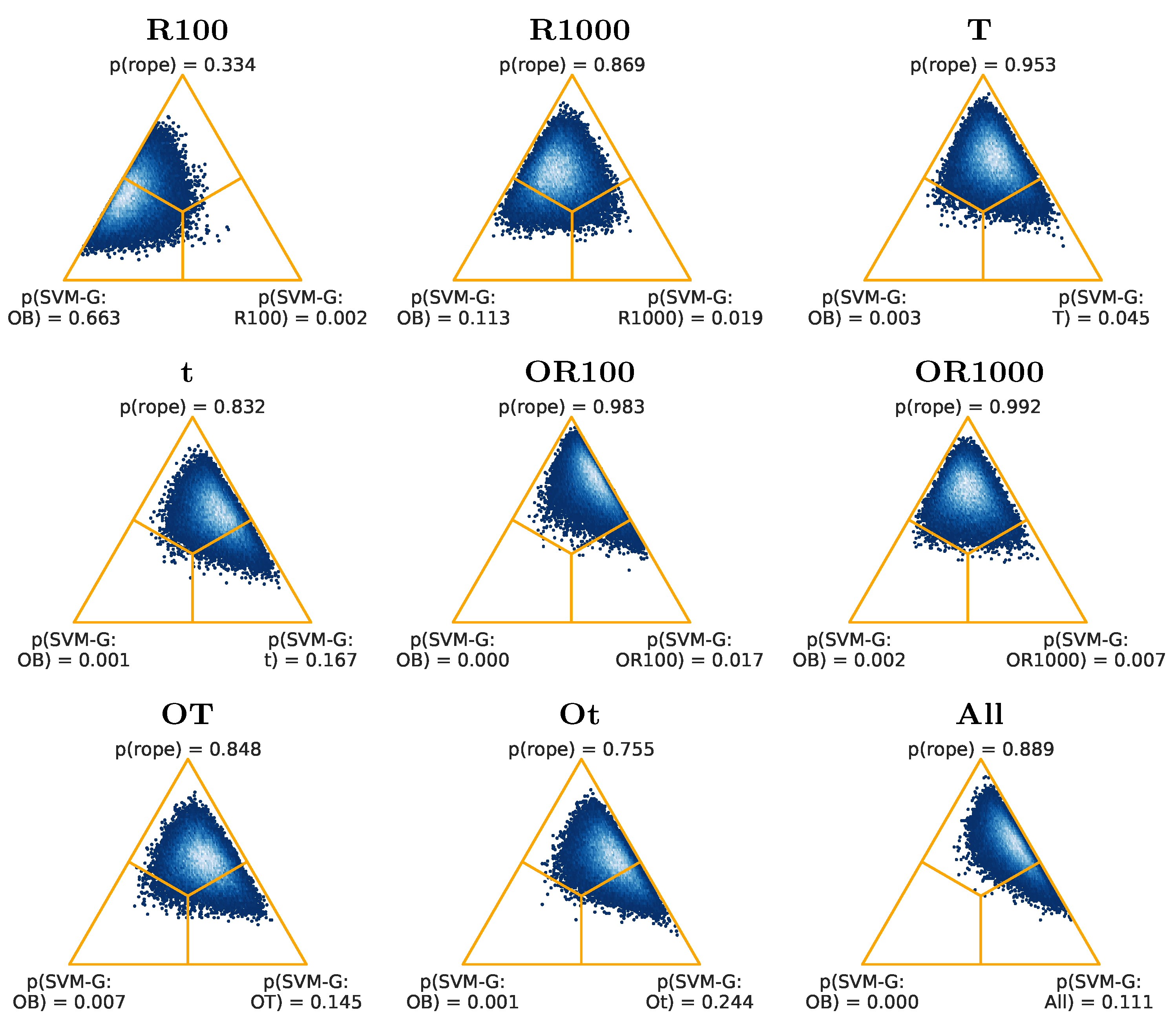
Figure 8, for SVM-G, the results are less favorable for the alternative cases to (OB). The best feature set is (Ot), with a probability of 0.244, being 0.001 the probability for (OB). The classification results for the three different classifiers therefore show an improvement that can be considered as significant, when using the different types of proposed feature sets, versus the features proposed in [18].

3.2. Results for the So-Called Difficult Datasets

An important part of the datasets reached a classification accuracy near or equal 100 % (Table A1, Table A2, Table A3 and Table A4, in Appendix A) , while others did not even reach 70 % . This was the reason we considered splitting up the dataset into two groups, one being formed only by what we may call the difficult datasets, for which the classification accuracy using SVM-L (best classifier in the previous work) was ≤90% using the original set of raw features. The list of difficult datasets (in Table A2) is the following: (1) Count 20 chips NO case x30 sorted; (2) Count 20 chips WITH case x30 sorted; (3) Count 20 papers x10; (4) Distance 3 mugs 10 distances; (5) Distance 3 mugs grouped by material; (6) Flip 10 creditcards NO case; (7) Identify 10 creditcards NO case; (8) Identify 5 colors x 20 chips; (9) Identify 6 users by palm; (10) Identify 6 users by touch behavior sorted; (11) Order 3 coasters NO case; (12) Order 3 creditcards NO case sorted; (13) Order 4 creditcards NO case sorted.
For the other datasets, simple methods may have good accuracy results, with little room for improvement. The entire experimental framework was repeated considering only this (difficult) subgroup of datasets, and the results are as follows.
Table 7 shows the average accuracies and average ranks, obtained using only the difficult datasets. The average accuracy for SVM-L:OB is 78.199 and for SVM-L:t is 87.173. The average rank of SVM-L:OB is 23.115 and 6.654 for SVM-L:All. Table 8 summarizes the results in Table 7 for each feature set, averaging the results of RF, SVM-L and SVM-G. The best feature set is (t), with an average accuracy of 85.58% and an average rank of 10.987. The average accuracy is 77.922 and the rank is 23.090 for (OB).
Given again the large number of methods (Classifier:Feature Set) tested, they were divided depending on the type of classifier used: RF, SVM-L, and SVM-G. These average ranks (for the difficult datasets) are shown in Table 9.
Figure 9 shows the critical difference diagrams for the Nemenyi test, for the three classifiers. The difference of the average ranks between RF:OB and the best feature sets with RF is greater than the critical difference. The distance of SVM-L:OB to the best feature sets with SVM-L is also greater. Nevertheless, the differences for SVM-G:OB and other feature sets with SVM-G are smaller than the critical difference.
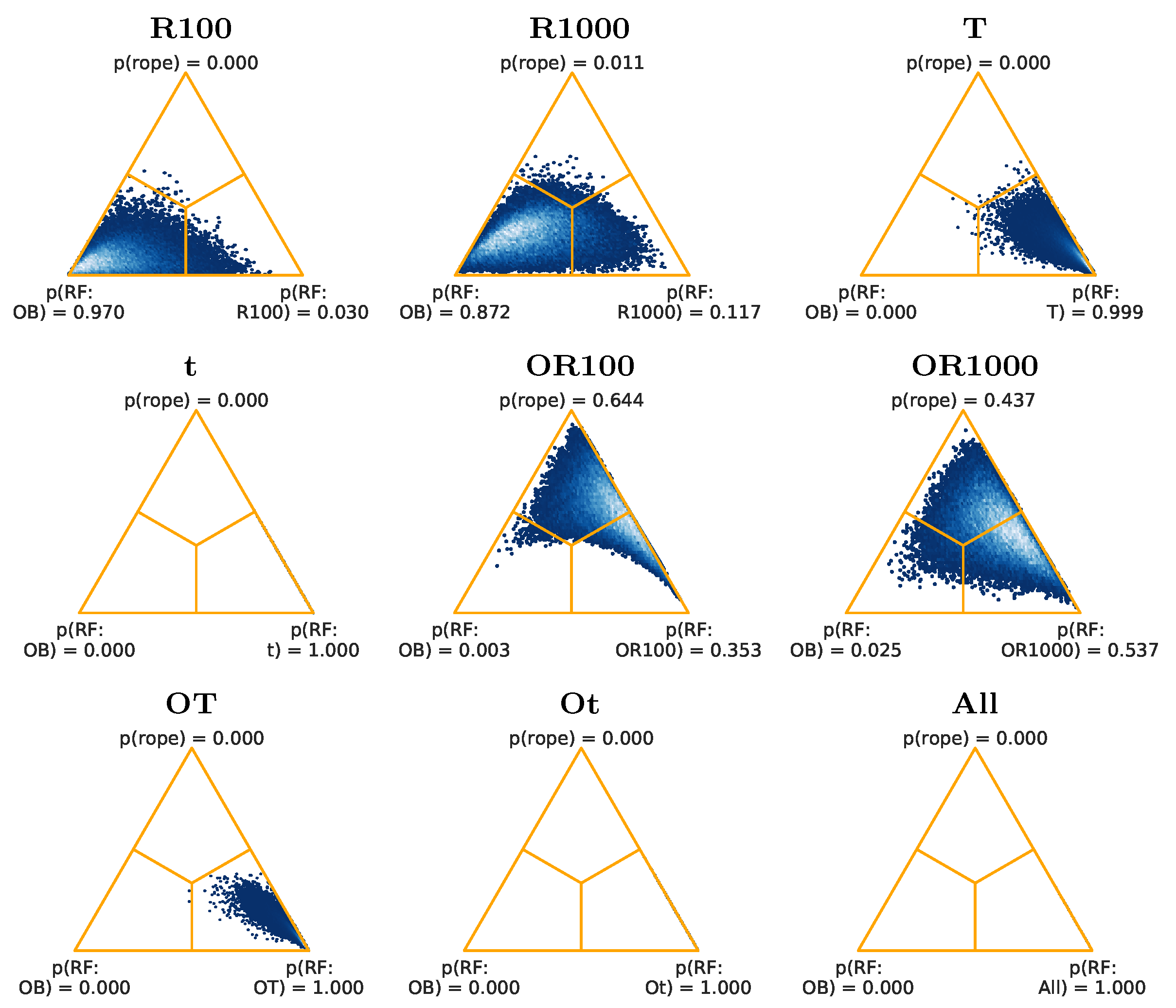
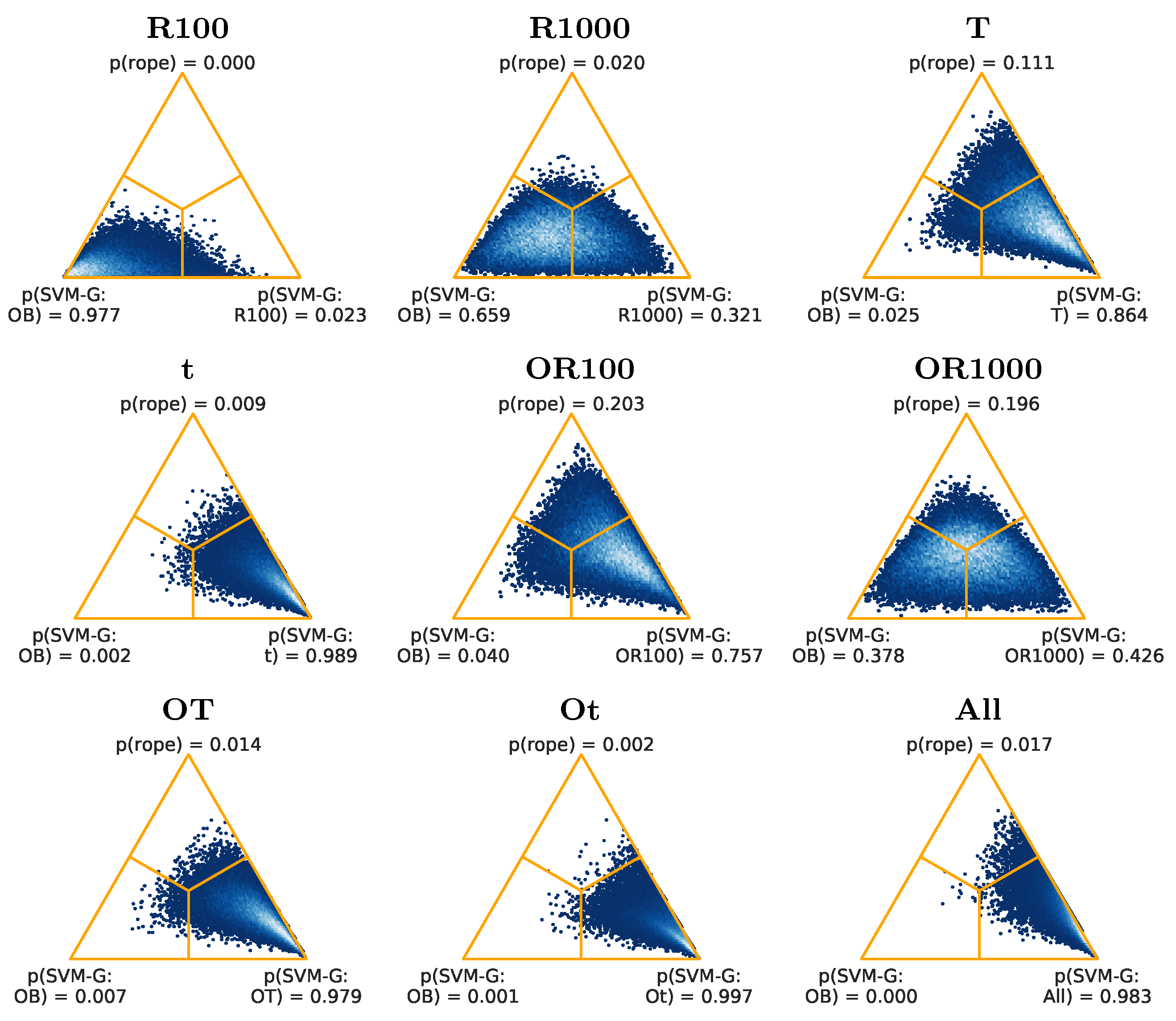
Figure 10, Figure 11 and Figure 12 show the Bayesian Signed-Rank Tests posteriors, for the RF, SVM-L, and SVM-G classifiers, respectively, for the difficult datasets. In 
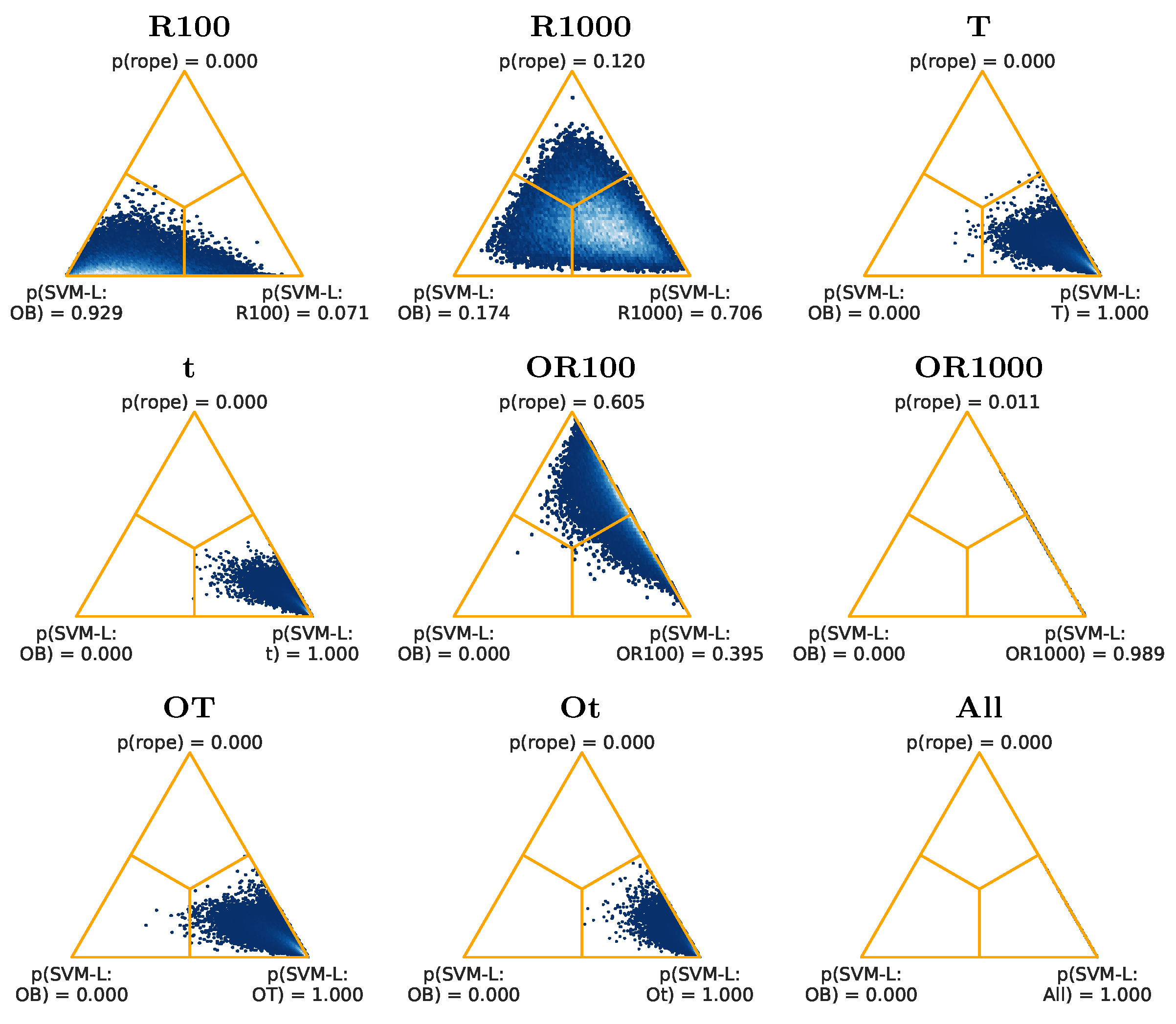
Figure 10, for RF, the feature sets with more favorable results when compared to (OB) are (t), (OT), (Ot), and (All), with a probability of 1.000 for the corresponding feature set, and 0.000 for (OB). For SVM-L (Figure 11), the best feature sets are, again, (t), (OT), (Ot), and (All), with a probability of 1.000 for the corresponding feature set, and 0.000 for (OB). In Figure 12, for SVM-G, the results are best for (Ot), with a probability of 0.997, and a probability of 0.001 for (OB), followed by (All), with a probability of 0.983, and a probability of 0.000 for (OB), and by (t), with a probability of 0.989, and a probability of 0.002 for (OB).

4. Conclusions

This paper presents a comparative analysis of different types of classification methodologies, applied on a series of datasets of raw signals acquired by a portable radar sensor, for different types of materials. In particular, twelve different types of feature vectors obtained from the original raw dataset were obtained, applying different types of feature extraction strategies. These feature vectors were subsequently combined with two classification methods (Random forests and SVM with linear and radial kernel types). A stacked generalization (Stacking) approach was also considered which involved base classifiers created using Random Forest and SVM trained using a subset of the different sets of features. The classification results shown outperformed the corresponding ones obtained by Shyong Yeo et al. [18], when considering the complete collection of datasets, as well as in a wider margin when using the partial so-called difficult datasets. In particular, the difference between the use of the TSFRESH with feature selection (t) features and the original and basic (OB) features (used in [18]), for the complete group of datasets, is almost 4 % in accuracy. Moreover, this difference increases to almost 7.7 % , for (t) vs. (OB) as well, for the so-called difficult subgroup.
From a classifier performance point-of-view, SVM with linear kernel (with default options) has the best global results (the methods with best average accuracy and rank in Table 4 and Table 7 use SVM-L), being much less costly than SVM with Gaussian kernel (with parameter adjustment) and Stacking. This suggest that it is not necessary to use expensive methods when using adequate feature extraction methods.
Potential future lines of research include the creation of our own datasets to explore the use of the radar sensor in problems that may have an industrial interest, for instance, in non-destructive testing or in the signal analysis of trash composites, to discern or classify them.

Author Contributions

J.F.D.-P., P.L.-C. and J.J.R. made the design of experiments, and carried them out. All the authors analysed the results and wrote the paper up. All authors have read and agreed to the published version of the manuscript.

Funding

This work was supported by the Spanish Ministry of Science and Innovation under project PID2020-119894GB-I00, Junta de Castilla y León under project BU055P20 (JCyL/FEDER, UE) co-financed through European Union FEDER funds. José Luis Garrido-Labrador was supported by the predoctoral grant (BDNS 510149) awarded by the Universidad de Burgos, Spain.

Institutional Review Board Statement

Not applicable.

Informed Consent Statement

Not applicable.

Data Availability Statement

Data and codes will be available upon demand.

Acknowledgments

We would like to thank the authors of [18] for making the datasets available (https://github.com/tcboy88/solinteractiondata (accessed on 18 January 2021). This work was supported by the Spanish Ministry of Science and Innovation under project PID2020-119894GB-I00, Junta de Castilla y León under project BU055P20 (JCyL/FEDER, UE) co-financed through European Union FEDER funds. José Luis Garrido-Labrador was supported by the predoctoral grant (BDNS 510149) awarded by the Universidad de Burgos, Spain.

Conflicts of Interest

Authors declare that they do not have any conflict of interests.

Appendix A. Tables with Classification Results for All Datasets

This section includes four tables corresponding to the complete classification results, for the 34 datasets, when applying RF, SVM-L, SVM-G, and Stacking classification strategies.
Table A1. Results for classifier RF with different feature sets.
OBOBTOTR100R1000tOtOR100OR1000All
Count + Order Lego97.0990.4596.0994.2797.0998.0098.0098.0097.0996.1898.0096.09
Count 20 chips NO case ×30 sorted65.6857.5763.6065.5166.9549.7657.2468.7066.9567.7465.1868.68
Count 20 chips WITH case ×30 sorted70.7961.1170.3273.3375.5666.9869.8475.2477.1472.0672.8675.71
Count 20 papers ×1078.5775.7175.7172.8673.3374.7676.6775.2475.2476.1977.1478.57
Distance 3 mugs 10 distances48.5652.7847.2267.8964.7875.1168.8978.6764.4449.6765.6773.22
Distance 3 mugs grouped by material71.3392.6784.3397.8999.0080.7880.00100.00100.0085.3384.11100.00
Distance 7 slotting100.0098.33100.00100.00100.00100.00100.00100.00100.00100.00100.00100.00
Flip 10 creditcards NO case82.2780.0083.6486.8285.0079.5579.5587.2786.3680.9183.6483.64
Flip 10 creditcards WITH case100.00100.00100.00100.00100.00100.00100.00100.00100.00100.00100.00100.00
Flip 52 cards94.3696.2796.1897.1897.2795.3697.2798.1898.1896.2797.1897.27
Identify 10 creditcards NO case85.4583.6487.2791.8290.9180.9185.4590.9191.8285.4583.6490.00
Identify 10 creditcards WITH case100.00100.00100.00100.00100.00100.00100.00100.00100.00100.00100.00100.00
Identify 12 printed designs100.00100.00100.00100.00100.00100.00100.00100.00100.00100.00100.00100.00
Identify 12 touch on numpad97.5691.6798.3397.8298.0896.1597.0597.9597.8298.2198.5998.46
Identify 5 colors × 20 chips75.0073.3375.4282.0881.2578.7580.8383.7583.3376.2582.0882.50
Identify 6 tagged plastic cards100.00100.00100.00100.00100.00100.00100.00100.00100.00100.00100.00100.00
Identify 6 users by palm82.8679.5282.8689.5289.0582.8685.2491.4390.9585.7185.2490.95
Identify 6 users by touch behavior sorted80.3871.4182.5695.2694.7473.2180.3897.6996.0382.9580.9094.49
Identify 7 dominoes96.25100.0098.75100.0098.7597.50100.0098.7598.7598.75100.00100.00
Identify 9 touch on half-sphere99.0094.6799.3398.0099.0096.0097.3398.1798.6798.3399.1799.00
Order 3 coasters NO case80.4271.2579.5885.4282.7176.2575.2182.9283.1380.2179.1783.33
Order 3 creditcards NO case sorted80.4069.0882.3980.4085.9973.2078.1284.2685.9982.3282.2885.40
Order 4 creditcards NO case sorted56.8543.5955.5156.4056.6947.3149.2556.1056.1055.9454.4759.07
Order 4 creditcards WITH case sorted99.4998.4699.4999.4999.4999.4999.4999.4999.4999.4999.4999.49
Rotation interval half numeric100.00100.00100.00100.00100.00100.00100.00100.00100.00100.00100.00100.00
Rotation interval one numeric99.17100.0099.17100.0099.17100.00100.00100.00100.0099.1799.17100.00
Slide inside-out on desk surface100.00100.00100.00100.00100.00100.00100.00100.00100.00100.00100.00100.00
Slide outside-in ruler100.00100.00100.00100.00100.00100.00100.00100.00100.00100.00100.00100.00
session1 × 1099.8199.2599.8199.8199.8199.81100.0099.8199.8199.8199.8199.62
session2 × 1099.2598.3099.6299.4399.4399.2599.4399.4399.4399.6299.4399.62
session3 × 1099.8199.6299.6299.8199.6299.8199.8199.8199.8199.8199.8199.62
session4 × 1099.8199.81100.00100.0099.81100.00100.0099.81100.00100.0099.81100.00
session5 × 1097.9297.5597.9298.6898.6897.5597.7498.6898.4998.1197.9298.49
session6 × 1099.2599.2599.2599.2599.2599.0699.0699.2599.2599.2599.2599.25
Mean89.3387.5189.8292.0392.1088.7589.7692.9392.4890.1190.7192.72
Average rank7.519.387.015.505.758.417.164.684.946.506.464.69
Table A2. Results for classifier SVM-L with different feature sets.
OBOBTOTR100R1000tOtOR100OR1000All
Count + Order Lego99.0096.0999.0096.0096.0098.0098.0096.0096.0099.0098.0097.00
Count 20 chips NO case ×30 sorted60.1160.4262.4971.7172.3560.9071.8872.3571.8769.1773.7873.94
Count 20 chips WITH case ×30 sorted79.5267.7879.5278.7379.3773.3378.8979.6880.0081.2781.2780.63
Count 20 papers ×1088.5779.5287.1482.3882.3888.1091.4384.2984.7688.1089.5286.19
Distance 3 mugs 10 distances39.1127.0047.5664.6761.3377.2280.5688.0072.2263.4475.1177.33
Distance 3 mugs grouped by material63.5677.0080.89100.00100.0090.4493.44100.00100.0085.2290.33100.00
Distance 7 slotting100.00100.00100.0098.33100.00100.00100.0098.33100.00100.00100.00100.00
Flip 10 creditcards NO case79.5575.4582.7386.8287.2779.5584.0988.1889.5582.7385.9188.64
Flip 10 creditcards WITH case100.0096.82100.00100.00100.00100.00100.00100.00100.00100.00100.00100.00
Flip 52 cards96.3692.4596.3698.1898.1897.0998.1899.0999.0994.3698.1898.18
Identify 10 creditcards NO case80.0081.8283.6488.1887.2779.0981.8290.0090.0083.6484.5586.36
Identify 10 creditcards WITH case100.00100.00100.0098.1898.18100.00100.00100.00100.00100.00100.00100.00
Identify 12 printed designs100.00100.00100.00100.00100.00100.00100.00100.00100.00100.00100.00100.00
Identify 12 touch on numpad99.3694.6298.9798.5998.8597.8297.9598.5998.5998.9798.7298.59
Identify 5 colors × 20 chips85.0076.6787.5094.5894.5881.2585.8396.6796.6787.0888.3396.67
Identify 6 tagged plastic cards100.00100.00100.0097.1497.14100.00100.00100.00100.00100.00100.00100.00
Identify 6 users by palm87.6285.7190.9592.8692.8686.1990.0095.2494.2990.0091.4395.24
Identify 6 users by touch behavior sorted82.1861.0385.3898.0897.9571.0385.6498.7298.7285.6488.7298.59
Identify 7 dominoes100.00100.00100.0096.2597.50100.00100.00100.00100.00100.00100.00100.00
Identify 9 touch on half-sphere97.5095.1798.6798.8398.8397.6799.5099.0099.0098.5099.6799.33
Order 3 coasters NO case82.9277.5081.0484.5885.4276.6780.0085.2185.2182.7183.1286.46
Order 3 creditcards NO case sorted82.3275.5986.5889.0189.0181.0784.1289.0190.2684.7487.8789.63
Order 4 creditcards NO case sorted60.1345.5461.1666.3666.3751.9358.6465.9167.4061.0160.7265.47
Order 4 creditcards WITH case sorted99.4999.2399.4999.4999.4999.4999.2399.4999.4999.4999.2399.49
Rotation interval half numeric100.00100.00100.0099.1799.17100.00100.00100.00100.00100.00100.00100.00
Rotation interval one numeric100.00100.00100.0099.1799.17100.00100.00100.00100.00100.00100.00100.00
Slide inside-out on desk surface100.00100.00100.0097.2797.27100.00100.00100.00100.00100.00100.00100.00
Slide outside-in ruler100.00100.00100.0098.1899.09100.00100.0099.0999.09100.00100.0099.09
session1 × 1099.8199.6299.8199.6299.62100.00100.0099.8199.8199.8199.8199.81
session2 × 1099.6299.0699.6298.8799.2599.6299.2599.0699.4399.6299.2599.43
session3 × 1099.8199.4399.8199.6299.6299.8199.8199.4399.6299.8199.8199.81
session4 × 10100.00100.00100.0099.6299.62100.00100.0099.4399.43100.00100.0099.43
session5 × 1098.8797.5598.4999.2599.2598.8799.2599.2599.2599.2599.2599.25
session6 × 1099.2599.2599.2599.2599.2599.0699.0699.2599.2599.2599.0699.25
Mean89.9987.0791.3593.2093.2890.7192.8494.6894.3892.1493.2894.52
Average rank6.969.436.417.666.967.436.295.535.066.005.514.76
Table A3. Results for classifier SVM-G with different feature sets.
OBOBTOTR100R1000tOtOR100OR1000All
Count + Order Lego98.0097.0098.0095.0995.0997.0098.0095.0995.0998.0098.0096.00
Count 20 chips NO case ×30 sorted71.3960.7471.2372.5073.9363.6073.6272.3574.2573.9473.4675.68
Count 20 chips WITH case ×30 sorted79.6869.6879.0579.5281.4375.4080.6380.9581.9083.3382.0681.75
Count 20 papers ×1088.5779.0587.6282.8683.3387.6290.0084.2983.8188.1089.0585.71
Distance 3 mugs 10 distances46.5658.0050.7863.6760.3377.2280.5688.0071.1162.5675.1177.33
Distance 3 mugs grouped by material71.3388.2280.89100.00100.0086.3392.44100.00100.0094.6788.33100.00
Distance 7 slotting100.00100.00100.0098.3396.67100.00100.0098.3398.33100.00100.0098.33
Flip 10 creditcards NO case87.2785.0088.1885.4586.3681.8285.4588.1887.7385.0085.4587.73
Flip 10 creditcards WITH case100.00100.00100.00100.00100.00100.00100.00100.00100.00100.00100.00100.00
Flip 52 cards98.1896.2798.1898.1898.1896.1898.1898.1898.1897.1896.1898.18
Identify 10 creditcards NO case90.0085.4584.5585.4586.3679.0983.6489.0988.1888.1883.6484.55
Identify 10 creditcards WITH case100.00100.00100.0099.0999.09100.00100.0099.0999.09100.00100.0099.09
Identify 12 printed designs100.0099.2399.23100.00100.00100.00100.00100.00100.00100.00100.0099.23
Identify 12 touch on numpad99.1096.1599.2398.3398.3397.8298.2198.4698.4698.8598.4698.46
Identify 5 colors × 20 chips86.6785.0088.3394.5894.5875.8385.0096.2596.2587.0887.5095.83
Identify 6 tagged plastic cards100.00100.00100.0098.5798.57100.00100.0098.5798.57100.00100.0098.57
Identify 6 users by palm89.5286.6791.9092.8691.9085.7189.5294.7693.3392.3890.4893.81
Identify 6 users by touch behavior sorted91.4182.0591.4197.8297.8282.9589.1098.4698.4691.9290.2698.08
Identify 7 dominoes100.0098.75100.0098.7598.75100.00100.0098.7598.75100.00100.0098.75
Identify 9 touch on half-sphere98.3397.0098.5098.8398.8398.3399.5099.0099.0099.0099.5099.33
Order 3 coasters NO case83.7576.0485.0085.0086.0476.2580.6385.4285.2183.5483.7586.04
Order 3 creditcards NO case sorted88.3878.1389.6389.6388.3879.8984.1587.7990.2687.7987.1789.04
Order 4 creditcards NO case sorted63.8451.4863.4066.5066.8153.2858.0466.6566.5163.0961.3266.06
Order 4 creditcards WITH case sorted99.2399.2399.2399.2399.2399.2399.2399.2399.2399.2399.2399.49
Rotation interval half numeric100.00100.00100.00100.0099.17100.00100.00100.00100.0099.1799.17100.00
Rotation interval one numeric99.1799.17100.0099.1799.17100.0099.17100.00100.00100.00100.00100.00
Slide inside-out on desk surface100.00100.00100.00100.00100.0099.0999.09100.00100.00100.0099.09100.00
Slide outside-in ruler100.00100.00100.0099.0999.09100.00100.0099.0999.09100.00100.0099.09
session1 × 1099.8199.6299.8199.6299.62100.00100.0099.8199.8199.8199.8199.81
session2 × 1099.6298.8799.2598.8799.0699.6299.0699.0699.2599.6299.4399.25
session3 × 1099.8199.4399.8199.4399.4399.8199.8199.4399.4399.8199.8199.62
session4 × 10100.00100.00100.0099.4399.62100.00100.0099.2599.25100.0099.8199.43
session5 × 1098.6897.9298.3099.0699.0698.8798.8799.0699.0699.0699.2598.87
session6 × 1099.2599.2599.2599.2599.2598.8799.0699.2599.2599.2599.0699.25
Mean91.9990.1092.3893.3693.3490.8892.9794.4794.0293.2593.0794.19
Average rank5.948.975.947.266.997.746.475.875.655.406.135.65
Table A4. Results for Stacking.
StackingStacking+
Count + Order Lego98.0098.00
Count 20 chips NO case ×30 sorted77.6076.17
Count 20 chips WITH case ×30 sorted80.9580.79
Count 20 papers ×1083.3383.81
Distance 3 mugs 10 distances64.7863.67
Distance 3 mugs grouped by material99.00100.00
Distance 7 slotting100.00100.00
Flip 10 creditcards NO case87.7386.82
Flip 10 creditcards WITH case100.00100.00
Flip 52 cards98.1898.18
Identify 10 creditcards NO case88.1888.18
Identify 10 creditcards WITH case100.00100.00
Identify 12 printed designs100.00100.00
Identify 12 touch on numpad98.9799.10
Identify 5 colors × 20 chips94.5896.25
Identify 6 tagged plastic cards100.00100.00
Identify 6 users by palm94.2995.24
Identify 6 users by touch behavior sorted98.4698.85
Identify 7 dominoes100.00100.00
Identify 9 touch on half-sphere98.8399.00
Order 3 coasters NO case82.0883.54
Order 3 creditcards NO case sorted88.3889.01
Order 4 creditcards NO case sorted64.4365.47
Order 4 creditcards WITH case sorted99.4999.49
Rotation interval half numeric100.00100.00
Rotation interval one numeric100.00100.00
Slide inside-out on desk surface100.00100.00
Slide outside-in ruler100.00100.00
session1 × 1099.8199.81
session2 × 1099.4399.43
session3 × 1099.8199.81
session4 × 1099.8199.81
session5 × 1098.4998.87
session6 × 1099.2599.25
Mean93.9494.07
Average rank1.601.40

References

  1. Stergiopoulos, S. Advanced Signal Processing Handbook: Theory and Implementation for Radar, Sonar, and Medical Imaging Real Time Systems; CRC Press: Boca Raton, FL, USA, 2000. [Google Scholar]
  2. Gini, F.; Rangaswamy, M. Knowledge-Based Radar Detection, Tracking, and Classification; John Wiley and Sons: Hoboken, NJ, USA, 2007. [Google Scholar]
  3. Ptak, P.; Hartikka, J.; Ritola, M.; Kauranne, T. Aircraft classification based on radar cross section of long-range trajectories. IEEE Trans. Aerosp. Electron. Syst. 2015, 51, 3099–3106. [Google Scholar] [CrossRef]
  4. Watts, S. Airborne Maritime Surveillance Radar, Volume 1; Morgan and Claypool Publishers: San Rafael, CA, USA, 2018; pp. 2053–2571. [Google Scholar] [CrossRef]
  5. Ajadi, O.A.; Barr, J.; Liang, S.Z.; Ferreira, R.; Kumpatla, S.P.; Patel, R.; Swatantran, A. Large-scale crop type and crop area mapping across Brazil using synthetic aperture radar and optical imagery. Int. J. Appl. Earth Obs. Geoinf. 2021, 97, 102294. [Google Scholar] [CrossRef]
  6. Spagnuolo, O.S.; Jarvey, J.C.; Battaglia, M.J.; Laubach, Z.M.; Miller, M.E.; Holekamp, K.E.; Bourgeau-Chavez, L.L. Mapping Kenyan Grassland Heights Across Large Spatial Scales with Combined Optical and Radar Satellite Imagery. Remote Sens. 2020, 12, 1086. [Google Scholar] [CrossRef] [Green Version]
  7. Lei, W.; Jiang, X.; Xu, L.; Luo, J.; Xu, M.; Hou, F. Continuous Gesture Recognition Based on Time Sequence Fusion Using MIMO Radar Sensor and Deep Learning. Electronics 2020, 9, 869. [Google Scholar] [CrossRef]
  8. Kang, S.W.; Jang, M.H.; Lee, S. Identification of Human Motion Using Radar Sensor in an Indoor Environment. Sensors 2021, 21, 2305. [Google Scholar] [CrossRef]
  9. Klavestad, S.; Assres, G.; Fagernes, S.; Grønli, T.M. Monitoring Activities of Daily Living Using UWB Radar Technology: A Contactless Approach. IoT 2020, 1, 320–336. [Google Scholar] [CrossRef]
  10. Park, D.; Lee, S.; Park, S.; Kwak, N. Radar-Spectrogram-Based UAV Classification Using Convolutional Neural Networks. Sensors 2021, 21, 210. [Google Scholar] [CrossRef] [PubMed]
  11. Kim, W.; Cho, H.; Kim, J.; Kim, B.; Lee, S. YOLO-Based Simultaneous Target Detection and Classification in Automotive FMCW Radar Systems. Sensors 2020, 20, 2897. [Google Scholar] [CrossRef]
  12. Senigagliesi, L.; Ciattaglia, G.; De Santis, A.; Gambi, E. People Walking Classification Using Automotive Radar. Electronics 2020, 9, 588. [Google Scholar] [CrossRef] [Green Version]
  13. Yeo, H.S.; Quigley, A. Radar sensing in human-computer interaction. Interactions 2017, 25, 70–73. [Google Scholar] [CrossRef] [Green Version]
  14. Wu, C.; Zhang, F.; Wang, B.; Liu, K.R. MSENSE: Towards mobile material sensing with a single millimeter-wave radio. Proc. ACM Interactive Mob. Wearable Ubiquitous Technol. 2020, 4, 1–20. [Google Scholar]
  15. Choi, J.W.; Ryu, S.J.; Kim, J.H. Short-Range Radar Based Real-Time Hand Gesture Recognition Using LSTM Encoder. IEEE Access 2019, 7, 33610–33618. [Google Scholar] [CrossRef]
  16. Hof, E.; Sanderovich, A.; Salama, M.; Hemo, E. Face Verification Using 802.11 waveforms. In Proceedings of the 2020 IEEE International Conference on Human-Machine Systems (ICHMS), Rome, Italy, 6–8 April 2020; pp. 1–4. [Google Scholar]
  17. Omer, A.E.; Safavi-Naeini, S.; Hughson, R.; Shaker, G. Blood glucose level monitoring using an FMCW millimeter-wave radar sensor. Remote Sens. 2020, 12, 385. [Google Scholar] [CrossRef] [Green Version]
  18. Yeo, H.S.; Minami, R.; Rodriguez, K.; Shaker, G.; Quigley, A. Exploring tangible interactions with radar sensing. Proc. ACM Interact. Mob. Wearable Ubiquitous Technol. 2018, 2, 1–25. [Google Scholar] [CrossRef] [Green Version]
  19. Ishii, H. Tangible bits: Beyond pixels. In Proceedings of the 2nd International Conference on Tangible and Embedded Interaction, Bonn, Germany, 18–20 February 2008. [Google Scholar]
  20. Breiman, L. Random forests. Mach. Learn. 2001, 45, 5–32. [Google Scholar] [CrossRef] [Green Version]
  21. Boser, B.E.; Guyon, I.M.; Vapnik, V.N. A Training Algorithm for Optimal Margin Classifiers. In Proceedings of the 5th Annual ACM Workshop on Computational Learning Theory, Pittsburgh, PA, USA, 27–29 July 1992; pp. 144–152. [Google Scholar]
  22. Wolpert, D.H. Stacked generalization. Neural Netw. 1992, 5, 241–259. [Google Scholar] [CrossRef]
  23. Dempster, A.; Petitjean, F.; Webb, G.I. ROCKET: Exceptionally fast and accurate time classification using random convolutional kernels. Data Min. Knowl. Discov. 2020. [Google Scholar] [CrossRef]
  24. Christ, M.; Braun, N.; Neuffer, J.; Kempa-Liehr, A.W. Time series feature extraction on basis of scalable hypothesis tests (tsfresh–a python package). Neurocomputing 2018, 307, 72–77. [Google Scholar] [CrossRef]
  25. Dau, H.A.; Bagnall, A.; Kamgar, K.; Yeh, C.C.M.; Zhu, Y.; Gharghabi, S.; Ratanamahatana, C.A.; Keogh, E. The UCR time series archive. IEEE/CAA J. Autom. Sin. 2019, 6, 1293–1305. [Google Scholar] [CrossRef]
  26. Bagnall, A.; Dau, H.A.; Lines, J.; Flynn, M.; Large, J.; Bostrom, A.; Southam, P.; Keogh, E. The UEA multivariate time series classification archive. arXiv 2018, arXiv:1811.00075. [Google Scholar]
  27. Bagnall, A.; Davis, L.; Hills, J.; Lines, J. Transformation based ensembles for time series classification. In Proceedings of the 2012 SIAM International Conference on Data Mining, Anaheim, CA, USA, 26–28 April 2012; pp. 307–318. [Google Scholar]
  28. Large, J.; Kemsley, E.K.; Wellner, N.; Goodall, I.; Bagnall, A. Detecting forged alcohol non-invasively through vibrational spectroscopy and machine learning. In Proceedings of the Pacific-Asia Conference on Knowledge Discovery and Data Mining, Melbourne, Australia, 3–6 June 2018; pp. 298–309. [Google Scholar]
  29. Ye, L.; Keogh, E. Time series shapelets: A new primitive for data mining. In Proceedings of the 15th ACM SIGKDD International Conference on Knowledge Discovery and Data Mining, Paris, France, 28 June–1 July 2009; pp. 947–956. [Google Scholar]
  30. Gandhi, A. Content-Based Image Retrieval: Plant Species Identification; Oregon State University: Corvallis, OR, USA, 2002. [Google Scholar]
  31. Lee, D.J.; Archibald, J.K.; Schoenberger, R.B.; Dennis, A.W.; Shiozawa, D.K. Contour matching for fish species recognition and migration monitoring. In Applications of Computational Intelligence in Biology; Springer: Berlin/Heidelberg, Germany, 2008; pp. 183–207. [Google Scholar]
  32. Christ, M.; Kempa-Liehr, A.W.; Feindt, M. Distributed and parallel time series feature extraction for industrial big data applications. arXiv 2016, arXiv:1610.07717. [Google Scholar]
  33. Benjamini, Y.; Yekutieli, D. The control of the false discovery rate in multiple testing under dependency. Ann. Stat. 2001, 29, 1165–1188. [Google Scholar] [CrossRef]
  34. Hsu, C.W.; Chang, C.C.; Lin, C.J. A Practical Guide to Support Vector Classification. 2003. Available online: http://www.datascienceassn.org/sites/default/files/Practical%20Guide%20to%20Support%20Vector%20Classification.pdf (accessed on 18 January 2021).
  35. Breiman, L. Bagging predictors. Mach. Learn. 1996, 24, 123–140. [Google Scholar] [CrossRef] [Green Version]
  36. Ho, T.K. C4.5 Decision Forests. In Proceedings of the 3rd International Conference on Document Analysis and Recognition, Montreal, QC, Canada, 14–16 August 1995; pp. 278–282. [Google Scholar]
  37. Garrido-Labrador, J.L.; Puente-Gabarri, D.; Ramírez-Sanz, J.M.; Ayala-Dulanto, D.; Maudes, J. Using Ensembles for Accurate Modelling of Manufacturing Processes in an IoT Data-Acquisition Solution. Appl. Sci. 2020, 10, 4606. [Google Scholar] [CrossRef]
  38. Prieto, O.J.; Alonso-González, C.J.; Rodríguez, J.J. Stacking for multivariate time series classification. Pattern Anal. Appl. 2015, 18, 297–312. [Google Scholar] [CrossRef]
  39. Garcia-Ceja, E.; Galván-Tejada, C.E.; Brena, R. Multi-view stacking for activity recognition with sound and accelerometer data. Inf. Fusion 2018, 40, 45–56. [Google Scholar] [CrossRef]
  40. Ouyang, Z.; Sun, X.; Chen, J.; Yue, D.; Zhang, T. Multi-view stacking ensemble for power consumption anomaly detection in the context of industrial internet of things. IEEE Access 2018, 6, 9623–9631. [Google Scholar] [CrossRef]
  41. Demšar, J. Statistical comparisons of classifiers over multiple data sets. J. Mach. Learn. Res. 2006, 7, 1–30. [Google Scholar]
  42. Benavoli, A.; Corani, G.; Mangili, F. Should we really use post-hoc tests based on mean-ranks? J. Mach. Learn. Res. 2016, 17, 152–161. [Google Scholar]
  43. Benavoli, A.; Corani, G.; Demšar, J.; Zaffalon, M. Time for a Change: A Tutorial for Comparing Multiple Classifiers Through Bayesian Analysis. J. Mach. Learn. Res. 2017, 18, 1–36. [Google Scholar]
  44. Nemenyi, P. Distribution-Free Mulitple Comparisons. Ph.D. Thesis, Princeton University, Princeton, NJ, USA, 1963. [Google Scholar]
Figure 1. Plots of the eight 64D signals (one 64D signal per channel) for two instances, each of a different dataset.
Applsci 11 06745 g001
Figure 2. Diagram of the Stacked Generalization approach.
Applsci 11 06745 g002
Figure 3. Flow chart describing the general data processing pipeline, divided into two steps.
Applsci 11 06745 g003
Figure 4. Boxplots of the differences in accuracy between the different feature sets and the feature set (OB), for the three considered classifiers. The boxplots on the right do not include the outliers. The average differences are marked with a red dot (•).
Applsci 11 06745 g004
Figure 5. Critical difference diagrams for the Nemenyi test ( α = 0.05 ).
Applsci 11 06745 g005
Figure 6. Posteriors for the Bayesian sign-rank tests for RF, from all the datasets.
Applsci 11 06745 g006
Figure 7. Posteriors for the Bayesian sign-rank tests for SVM-L, from all the datasets.
Applsci 11 06745 g007
Figure 8. Posteriors for the Bayesian sign-rank tests for SVM-G, from all the datasets.
Applsci 11 06745 g008
Figure 9. Critical difference diagrams for the Nemenyi test, for the difficult datasets ( α = 0.05 ).
Applsci 11 06745 g009
Figure 10. Posteriors for the Bayesian sign-rank tests for RF, from the difficult datasets.
Applsci 11 06745 g010
Figure 11. Posteriors for the Bayesian sign-rank tests for SVM-L, from the difficult datasets.
Applsci 11 06745 g011
Figure 12. Posteriors for the Bayesian sign-rank tests for SVM-G, from the difficult datasets.
Applsci 11 06745 g012
Table 1. Columns show radar datasets used, including the problem type (C, Counting; M, Material Identification; D, Distance estimation; O, Order identification; F, Flipping identification (Up/Down)); I, Object identification; R, Movement, rotation; P, Movement, position), the total number of samples, and the number of classes for each dataset.
DatasetProblem# of Samples# of Classes
1Count + Order LegoC10611
2Count 20 chips NO case x30 sortedC62921
3Count 20 chips WITH case x30 sortedC63021
4Count 20 papers x10C21021
5Distance 3 mugs 10 distancesM + D9331
6Distance 3 mugs grouped by materialM934
7Distance 7 slottingD608
8Flip 10 creditcards NO caseF + I22021
9Flip 10 creditcards WITH caseF + I22021
10Flip 52 cardsF1053
11Identify 10 creditcards NO caseI11011
12Identify 10 creditcards WITH caseI11011
13Identify 12 printed designsI13013
14Identify 12 touch on numpadI78013
15Identify 5 colors × 20 chipsI2406
16Identify 6 tagged plastic cardsI707
17Identify 6 users by palmI2107
18Identify 6 users by touch behavior sortedI7807
19Identify 7 dominoesI808
20Identify 9 touch on half-sphereI60010
21Order 3 coasters NO caseO48016
22Order 3 creditcards NO case sortedO16416
23Order 4 creditcards NO case sortedO67265
24Order 4 creditcards WITH case sortedO39065
25Rotation interval half numericR12012
26Rotation interval one numericR12012
27Slide inside-out on desk surfaceP11011
28Slide outside-in rulerP11011
29session1 × 10C53053
30session2 × 10C53053
31session3 × 10C53053
32session4 × 10C53053
33session5 × 10C53053
34session6 × 10C53053
Table 2. Combination of features used, including their total number. In the case of variable-size feature extraction methods, the minimum, maximum, and average values, respectively, are also given (in parenthesis).
FeaturesAbbreviationNo of Attributes
Raw Original Data(O)512
Basic aggregation features(B)149
ROCKET with 100 kernels(R100)200
ROCKET with 1000 kernels(R1000)2000
TSFRESH without feature selection(T)6352
TSFRESH with feature selection(t)Variable (885/3567/3235)
Original & Basic(OB)661
Original & ROCKET (100)(OR100)712
Original & ROCKET (1000)(OR1000)2512
Original & TSFRESH (without feat. sel.)(OT)6864
Original & TSFRESH (with feat. sel.)(Ot)Variable (1397/4079/3747)
Original, basic, ROCKET (1000) and TSFRESH (with feat. sel.)(All)Variable (3546/6228/5896)
Table 3. Results for a subset of the classifiers with different feature sets.
RF:OBRF:OtSVM-L:R1000SVM-L:tSVM-L:OBSVM-L:OR1000SVM-L:OtSVM-L:AllSVM-G:R1000SVM-G:OBSVM-G:OR100Stack:AllStack+:All
Count + Order Lego96.0997.0998.0096.0099.0098.0096.0097.0098.0098.0098.0098.0098.00
Count 20 chips NO case ×30 sorted63.6066.9571.8872.3562.4973.7871.8773.9473.6271.2373.9477.6076.17
Count 20 chips WITH case ×30 sorted70.3277.1478.8979.6879.5281.2780.0080.6380.6379.0583.3380.9580.79
Count 20 papers ×1075.7175.2491.4384.2987.1489.5284.7686.1990.0087.6288.1083.3383.81
Distance 3 mugs 10 distances47.2264.4480.5688.0047.5675.1172.2277.3380.5650.7862.5664.7863.67
Distance 3 mugs grouped by material84.33100.0093.44100.0080.8990.33100.00100.0092.4480.8994.6799.00100.00
Distance 7 slotting100.00100.00100.0098.33100.00100.00100.00100.00100.00100.00100.00100.00100.00
Flip 10 creditcards NO case83.6486.3684.0988.1882.7385.9189.5588.6485.4588.1885.0087.7386.82
Flip 10 creditcards WITH case100.00100.00100.00100.00100.00100.00100.00100.00100.00100.00100.00100.00100.00
Flip 52 cards96.1898.1898.1899.0996.3698.1899.0998.1898.1898.1897.1898.1898.18
Identify 10 creditcards NO case87.2791.8281.8290.0083.6484.5590.0086.3683.6484.5588.1888.1888.18
Identify 10 creditcards WITH case100.00100.00100.00100.00100.00100.00100.00100.00100.00100.00100.00100.00100.00
Identify 12 printed designs100.00100.00100.00100.00100.00100.00100.00100.00100.0099.23100.00100.00100.00
Identify 12 touch on numpad98.3397.8297.9598.5998.9798.7298.5998.5998.2199.2398.8598.9799.10
Identify 5 colors × 20 chips75.4283.3385.8396.6787.5088.3396.6796.6785.0088.3387.0894.5896.25
Identify 6 tagged plastic cards100.00100.00100.00100.00100.00100.00100.00100.00100.00100.00100.00100.00100.00
Identify 6 users by palm82.8690.9590.0095.2490.9591.4394.2995.2489.5291.9092.3894.2995.24
Identify 6 users by touch behavior sorted82.5696.0385.6498.7285.3888.7298.7298.5989.1091.4191.9298.4698.85
Identify 7 dominoes98.7598.75100.00100.00100.00100.00100.00100.00100.00100.00100.00100.00100.00
Identify 9 touch on half-sphere99.3398.6799.5099.0098.6799.6799.0099.3399.5098.5099.0098.8399.00
Order 3 coasters NO case79.5883.1380.0085.2181.0483.1285.2186.4680.6385.0083.5482.0883.54
Order 3 creditcards NO case sorted82.3985.9984.1289.0186.5887.8790.2689.6384.1589.6387.7988.3889.01
Order 4 creditcards NO case sorted55.5156.1058.6465.9161.1660.7267.4065.4758.0463.4063.0964.4365.47
Order 4 creditcards WITH case sorted99.4999.4999.2399.4999.4999.2399.4999.4999.2399.2399.2399.4999.49
Rotation interval half numeric100.00100.00100.00100.00100.00100.00100.00100.00100.00100.0099.17100.00100.00
Rotation interval one numeric99.17100.00100.00100.00100.00100.00100.00100.0099.17100.00100.00100.00100.00
Slide inside-out on desk surface100.00100.00100.00100.00100.00100.00100.00100.0099.09100.00100.00100.00100.00
Slide outside-in ruler100.00100.00100.0099.09100.00100.0099.0999.09100.00100.00100.00100.00100.00
session1 × 1099.8199.81100.0099.8199.8199.8199.8199.81100.0099.8199.8199.8199.81
session2 × 1099.6299.4399.2599.0699.6299.2599.4399.4399.0699.2599.6299.4399.43
session3 × 1099.6299.8199.8199.4399.8199.8199.6299.8199.8199.8199.8199.8199.81
session4 × 10100.00100.00100.0099.43100.00100.0099.4399.43100.00100.00100.0099.8199.81
session5 × 1097.9298.4999.2599.2598.4999.2599.2599.2598.8798.3099.0698.4998.87
session6 × 1099.2599.2599.0699.2599.2599.0699.2599.2599.0699.2599.2599.2599.25
Mean89.8292.4892.8494.6891.3593.2894.3894.5292.9792.3893.2593.9494.07
Table 4. Average accuracies and ranks from all the datasets.
MethodAccuracyMethodRank
SVM-L:t94.678SVM-L:All12.632
SVM-L:All94.524Stacking+:All12.676
SVM-G:t94.466SVM-L:Ot13.456
SVM-L:Ot94.382Stacking:All14.265
SVM-G:All94.188SVM-L:t14.853
Stacking+:All94.075SVM-L:OR100015.368
SVM-G:Ot94.025SVM-G:OR10015.441
Stacking:All93.938SVM-G:O16.824
SVM-G:T93.359SVM-L:OR10016.971
SVM-G:OT93.338SVM-G:OB17.176
SVM-L:OR100093.283SVM-G:All17.309
SVM-L:OT93.283SVM-L:R100017.338
SVM-G:OR10093.252SVM-G:OR100017.588
SVM-L:T93.205SVM-G:Ot17.662
SVM-G:OR100093.070RF:t17.794
SVM-G:R100092.969SVM-G:t17.853
RF:t92.926SVM-L:OB18.132
SVM-L:R100092.840RF:All18.176
RF:All92.720SVM-G:R100018.265
RF:Ot92.479RF:Ot18.353
SVM-G:OB92.375RF:T19.279
SVM-L:OR10092.141SVM-L:O19.603
RF:OT92.100SVM-L:OT20.176
RF:T92.028RF:OT20.426
SVM-G:O91.987SVM-L:R10021.044
SVM-L:OB91.355SVM-G:OT21.103
SVM-G:R10090.877SVM-G:T21.382
SVM-L:R10090.712SVM-L:T21.544
RF:OR100090.706RF:OR100021.779
RF:OR10090.110SVM-G:R10022.765
SVM-G:B90.100RF:OR10022.897
SVM-L:O89.989RF:OB23.176
RF:OB89.823RF:R100023.338
RF:R100089.761RF:O24.706
RF:O89.333RF:R10025.971
RF:R10088.747SVM-G:B26.603
RF:B87.508SVM-L:B28.088
SVM-L:B87.068RF:B28.985
Table 5. Average accuracies and ranks for each feature set, from all the datasets. For each feature set, the values in these tables are the averages for RF, SVM-L, and SVM-G in Table 4.
Feature SetAccuracyFeature SetRank
t94.024All16.039
All93.811Ot16.490
Ot93.628t16.833
OT92.907OR100018.245
T92.864OR10018.436
OR100092.353OB19.495
R100091.857R100019.647
OR10091.834O20.377
OB91.184OT20.569
O90.437T20.735
R10090.112R10023.260
B88.226B27.892
Table 6. Average ranks for each classification method.
RFSVM-LSVM-G
MethodRankMethodRankMethodRank
RF:t4.676SVM-L:All4.765SVM-G:OR1005.397
RF:All4.691SVM-L:Ot5.059SVM-G:Ot5.647
RF:Ot4.941SVM-L:OR10005.515SVM-G:All5.647
RF:T5.500SVM-L:t5.529SVM-G:t5.868
RF:OT5.750SVM-L:OR1006.000SVM-G:O5.941
RF:OR10006.456SVM-L:R10006.294SVM-G:OB5.941
RF:OR1006.500SVM-L:OB6.412SVM-G:OR10006.132
RF:OB7.015SVM-L:O6.956SVM-G:R10006.471
RF:R10007.162SVM-L:OT6.956SVM-G:OT6.985
RF:O7.515SVM-L:R1007.426SVM-G:T7.265
RF:R1008.412SVM-L:T7.662SVM-G:R1007.735
RF:B9.382SVM-L:B9.426SVM-G:B8.971
Table 7. Average accuracies and ranks from the difficult datasets .
MethodAccuracyMethodRank
SVM-L:t87.173SVM-L:All6.654
SVM-G:t87.092SVM-L:Ot7.154
SVM-L:All86.550SVM-L:t7.538
SVM-G:All86.278SVM-G:t7.731
SVM-L:Ot86.226SVM-G:Ot7.846
SVM-G:Ot85.924SVM-G:All8.308
Stacking+:All85.215Stacking+:All9.577
Stacking:All84.908Stacking:All11.654
SVM-L:T84.458SVM-G:OT11.808
SVM-G:OT84.407SVM-L:OT12.654
SVM-L:OT84.319SVM-L:T13.077
SVM-G:T84.297SVM-G:T13.500
SVM-G:OR10083.199SVM-G:OR10014.462
SVM-L:OR100083.128SVM-L:OR100015.115
SVM-G:OR100082.891SVM-G:OR100015.654
SVM-G:R100082.522SVM-G:OB16.423
RF:t82.475SVM-G:O17.462
SVM-L:R100082.026RF:t17.692
RF:All81.967SVM-G:R100018.077
RF:Ot81.345RF:All19.000
SVM-G:OB80.921RF:Ot19.346
RF:OT80.458SVM-L:R100019.885
RF:T80.400SVM-L:OR10020.808
SVM-L:OR10080.365RF:T20.808
SVM-G:O79.875RF:OT22.115
SVM-L:OB78.199SVM-L:OB23.115
SVM-G:R10077.307SVM-L:O27.115
SVM-L:R10076.674SVM-L:R10027.885
RF:OR100076.643SVM-G:R10028.077
SVM-G:B75.809RF:OR10028.846
RF:OR10075.442SVM-G:B28.923
SVM-L:O74.660RF:OR100029.000
RF:OB74.647RF:OB29.731
RF:R100074.360RF:O30.154
RF:O73.736RF:R100031.731
RF:R10072.264RF:R10033.538
RF:B70.128RF:B34.231
SVM-L:B68.541SVM-L:B34.308
Table 8. Average accuracies and ranks for each feature set, from the difficult datasets. For each feature set, the values in these tables are the averages for RF, SVM-L, and SVM-G in Table 7.
Feature SetAccuracyFeature SetRank
t85.580t10.987
All84.932All11.321
Ot84.498Ot11.449
OT83.062OT15.526
T83.051T15.795
OR100080.887OR100019.923
OR10079.669OR10021.372
R100079.636OB23.090
OB77.922R100023.231
O76.090O24.910
R10075.415R10029.833
B71.492B32.487
Table 9. Average ranks for each classification method, for difficult datasets.
RFSVM-LSVM-G
MethodRankMethodRankMethodRank
RF:t2.808SVM-L:All2.923SVM-G:Ot3.308
RF:All2.923SVM-L:Ot3.192SVM-G:t3.577
RF:Ot3.538SVM-L:t3.346SVM-G:All3.808
RF:OT4.692SVM-L:OT4.885SVM-G:OT5.000
RF:T4.731SVM-L:OR10005.231SVM-G:T6.000
RF:OR1006.962SVM-L:T5.423SVM-G:OR1006.192
RF:OR10007.346SVM-L:R10007.154SVM-G:OB6.962
RF:O7.692SVM-L:OR1007.231SVM-G:OR10007.000
RF:OB8.000SVM-L:OB7.923SVM-G:O7.269
RF:R10008.846SVM-L:O9.385SVM-G:R10007.692
RF:R10010.038SVM-L:R1009.692SVM-G:R10010.308
RF:B10.423SVM-L:B11.615SVM-G:B10.885
Publisher’s Note: MDPI stays neutral with regard to jurisdictional claims in published maps and institutional affiliations.

