Employing a Long-Short-Term Memory Neural Network to Improve Automatic Sleep Stage Classification of Pharmaco-EEG Profiles

Abstract

An increasing problem in today’s society is the spiraling number of people suffering from various sleep disorders. The research results presented in this paper support the use of a novel method that employs techniques from the classification of sleep disorders for more accurate scoring. Applying this novel method will assist researchers with better analyzing subject profiles for recommending prescriptions or to alleviate sleep disorders. In biomedical research, the use of animal models is required to experimentally test the safety and efficacy of a drug in the pre-clinical stage. We have developed a novel LSTM Recurrent Neural Network to process Pharmaco-EEG Profiles of rats to automatically score their sleep–wake stages. The results indicate improvements over the current methods; for the case of combined channels, the model accuracy improved by 1% and 3% in binary or multiclass classifications, respectively, to accuracies of 93% and 82%. In the case of using a single channel, binary and multiclass LSTM models for identifying rodent sleep stages using single or multiple electrode positions for binary or multiclass problems have not been evaluated in prior literature. The results reveal that single or combined channels, and binary or multiclass classification tasks, can be applied in the automatic sleep scoring of rodents.

1. Introduction

Sleep is important to both humans and animals. Sleep disorders are increasing and are grouped into anxiety, insomnia, sleep related movement disorders, etc. [1]. Benzodiazepines are recommended for the treatment of sleep disorders on a short-term basis [2], but their long-term use risks addiction and dependence. Furthermore, the side effects include decreased perceptual-motoric performance, disturbed EEG patterns during sleep, and dependence, among others. Hypnotic and anxiolytic drugs are required, such that do not produce dependence or other serious adverse effects. The Lavender EO (essential oil) has a long history of therapeutic use and does have anxiolytic properties. It is widely utilized by rural populations all over the world. According to Persian medicine protocol, lavender is beneficial in the treatment of chronic respiratory ailments.

EEG is an examination technique to measure brain activity and allows for identifying the sleep stages from a polysomnographic recording [3]. An EMG is useful for diagnostics of the neck muscles. Polysomnography (PSG) is used to analyze and diagnose sleep health. In a sleep center, the patient’s overnight sleep activity is recorded in the form of PSG recordings. A PSG is a set of bio-signals such as respiratory signals, electroencephalography (EEG), electrooculogram (EOG), electromyogram (EMG), and electrocardiogram (ECG). The system by which the EEG electrodes are applied to the head and the display of the EEG record is called the international 10–20 system [4]. A human sleep analyst visually inspects every 30 s epoch of the sleep data, and manually assigns a score to each type of signal. Manually, three sleep stages are defined, namely Wake, Random Eye Movement (REM), and Non-Random eye movement (NREM) [5]. It is essential to have sleep stage information for diagnosing sleep related problems.

The manual sleep scoring is a tedious task and the results can be perturbed by loss of concentration, and they also depend on various other factors such as data quality, artifacts, sleep fragmentation, etc [6]. Sleep experts take up to 3 h in order to score 24 h of EEG/EMG recordings, whereas to score the same amount of data, novice staff may take up to 6 h. Sleep related studies have a challenge in achieving high data quality and in establishing long-term studies with internal consistency [7].

Sleep scoring takes advantage of machine learning techniques to overcome the afore-mentioned issues. Automated sleep scoring relies on feature engineering in order to create classifier models. The feature engineering approach necessitates professional expertise and may not produce characteristics that are optimal for sleep scoring. Deep Learning (DL) takes a huge amount of data and new methods to automate the sleep annotation process.

We propose a trainable LSTM model for detecting sleep stages in rodents. The advantage of the LSTM method is that it is effective and has performed well for long time-series data [8]. It learns to recognize the next possible sleep stage among the consecutive stages. To generate Pharmaco-EEG profiles and sleep patterns, lavender EO was used in vivo to treat a rat model.

We studied the effectiveness of single or multiple electrode positions for rodent sleep stage classification. The main purpose was twofold: to reduce the computational complexity of signal processing by selecting the relevant channels, and to reduce the amount of overfitting that may arise due to unnecessary channels. Secondly, multiclass classification problems are challenged by imbalanced data, which causes problems for several ML algorithms. Therefore, a related binary classification problem was posed along with the multiclass one, in order to assess the comparative effectiveness of these approaches in the identification of rodent sleep stage combinations.

2. Related Work

A number of rat sleep scoring methods have been proposed. Kohn introduced the first algorithm for rodent sleep stage scoring [9]. In most of the existing methods, a subset of data for each subject’s sleep stage analysis is prepared with human interaction to identify wake-sleep state cut-off or to perform manual sleep scoring, but the employed techniques or methods can differ. Manual sleep scoring is annotated by the sleep expert, whereas machine and deep learning models have the ability to classify the sleep stages automatically without intervention by a human. The conventional sleep scoring methods extract frequency domain features by employing the fast Fourier transform [10,11,12].

In contrast, in unsupervised learning, the sleep stages are discriminated by using rules, possibly embedded in a trained artificial neural network or in a Bayes net. Few unsupervised algorithms have been proposed, but they can be computationally intensive and have only been tested on a limited number of animals. The various classification models used to handle features and sleep stages include Support Vector Machines [11], Hidden Markov Model, and LSTM (which is designed for time series and employs sleep transition rules to obtain a high level of accuracy) [13].

Numerous studies have pursued automated sleep scoring. The authors [14] proposed MC-SleepNet, which is based on the convolutional neural network and long-short-term memory (LSTM) and attained 96.6% accuracy. Another author [8] introduced a convolutional neural network (CNN) architecture for automated sleep scoring in mice and accomplished an F1-Score of 0.95. The study [15] compared machine and deep learning models for automated sleep scoring of rodents, both mice and rats. They obtained accuracies within 0.77–0.83 for the rodent with a convolutional neural network (that was compared to Random Forest (0.78–0.81)). Another approach known as sleep scoring artificial neural network for rodents achieved 96.8% accuracy [16].

To the best of our knowledge, numerous studies have discussed sleep stage classification accuracy, but the relationship between the sleep stages and model performance is not discussed. Furthermore, the effect of electrode position on model performance is not dealt with in the literature. A hybrid approach combining CNN and LSTM for automatic sleep stage classification is discussed in [17].

In order to fill the gap, we have employed the LSTM neural network to improve the classification accuracy of binary or multiple sleep stages, along with comparison of single or multiple electrode positions.

3. Experimental Setup

In this section, we will explain the steps in experimentation with a particular focus on the data collected and how it was used.

3.1. Data Collection

A description on the subjects identified for the study is presented. In addition, the data acquisition processes are explained in Section 3.2.

3.1.1. Subjects

The subjects were 6 male Wistar rats of weights 250–300 g in the Southern Laboratory Animal Facility, Prince of Songkla University, Songkhla, Thailand. They were fed commercial food pellets and provided water. The tests were conducted in the hours between 9:00 a.m. and 3:00 p.m. The work adhered to the European Science Foundation’s (ESF) (Use of Animals in Research, 2001) and the International Committee on Laboratory Animal Science’s (ICLAS) ethical guidelines (2004). The Animal Ethical Committee of the Prince of Songkla University (MOE 0521.11/613) approved and guided the experimental methodology.

3.1.2. EEG Electrode Implantation

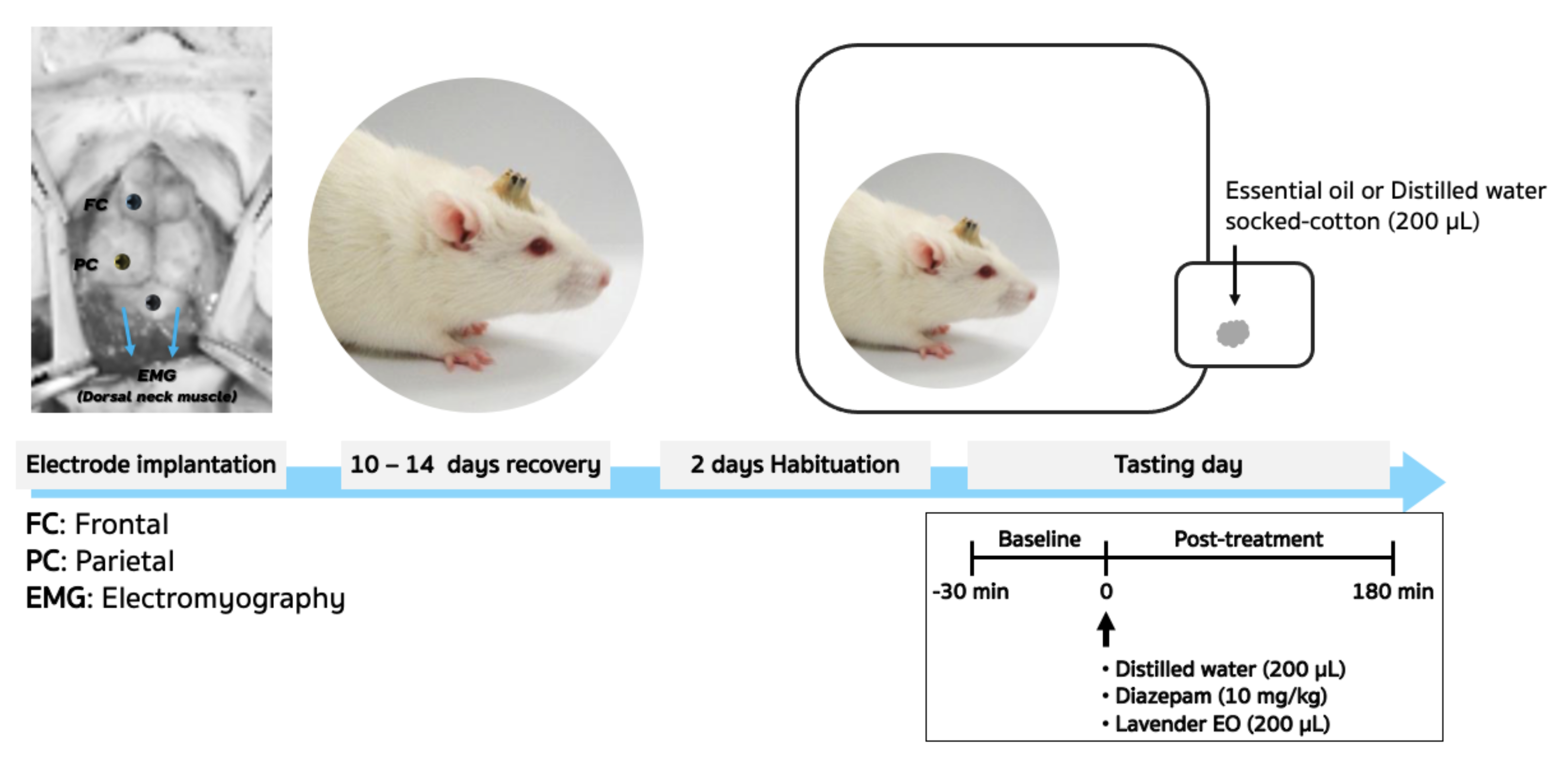
Pre-injection of 60 mg/kg Zoletil 100 intramuscularly sedated the animals. According to the bregma of the rat brain atlas, see Figure 1, a set of screw electrodes made of stainless steel were implanted on the frontal (AP; +3 mm, ML; 3 mm) and left side of the skull in the parietal cortex (AP; −4 mm, ML; 4 mm). The reference and ground electrodes were placed at the midline over cerebellum [4]. For electromyography (EMG), bipolar electrodes were implanted in the dorsal neck muscles. To avoid infection, the antibiotic ampicillin (General Drug House Co., Ltd., Bangkok, Thailand) was given intramuscularly (100 mg/kg) once a day for three days, and the subjects were permitted at least ten days to recover completely.

3.2. Data Acquisition Process

The animals were acclimatized to the experimental circumstances in the inhalation chamber for two days after they had fully recovered from surgery before being tested. The animals were subjected to the same conditions as the habituation days during the testing days, and their EEGs were recorded. Baseline activity was monitored for 30 min before treatment. Animals were divided into three groups to receive the inhalation of either 200 microliters of lavender EO or 200 microliters of distilled water (control), or an intraperitoneal injection of 15 mg/kg diazepam (positive control). Post-drug recording was performed for 180 min after treatment. Values of EEG parameters were normalized with baseline levels and are expressed in % baseline. The overall experimental protocol setup for EEG recording is shown in Figure 1.

An airtight cylindrical plastic chamber was used as the inhaling chamber. The diameter was 25 cm, and the length was 50 cm (height). It was perforated with two small openings for intake and outlet (opposite to each other) having air tubing connections. The inlet tubing was connected to a fan delivering ambient air and/or volatile molecules into the chamber. The outlet tubing was for outflow ventilation. The fan engine was powered by direct current and required 1.92 W of electricity. The rotation speed was 4000 rpm with an air flow of 0.41 cmm (cubic meters per minute).

EEG and EMG Signal Acquisition

EEG and EMG signals were collected with low-pass 50 Hz and high-pass 0.1 Hz filters, and were sampled at 400 Hz by a PowerLab/4SP system (AD Instruments) with 12-bit A/D, and then stored in a PC through the LabChart 7 software. The EEG and EMG signals were handled using band-pass digital filters that ranged from 0.78 to 45.31 Hz and from 1 to 100 Hz, respectively. Standard LFP analysis, the frequency analysis, was performed using the Fast Fourier transform (FFT) function in LabChart 7.

3.3. Data Pre-Processing

The process of noise removal and data scaling is explained in this section.

3.3.1. Noise Removal

In order to remove the noise from sleep EEG signals, we applied a Butterworth low-pass filter. A sample of filtered data is shown in Figure 2.

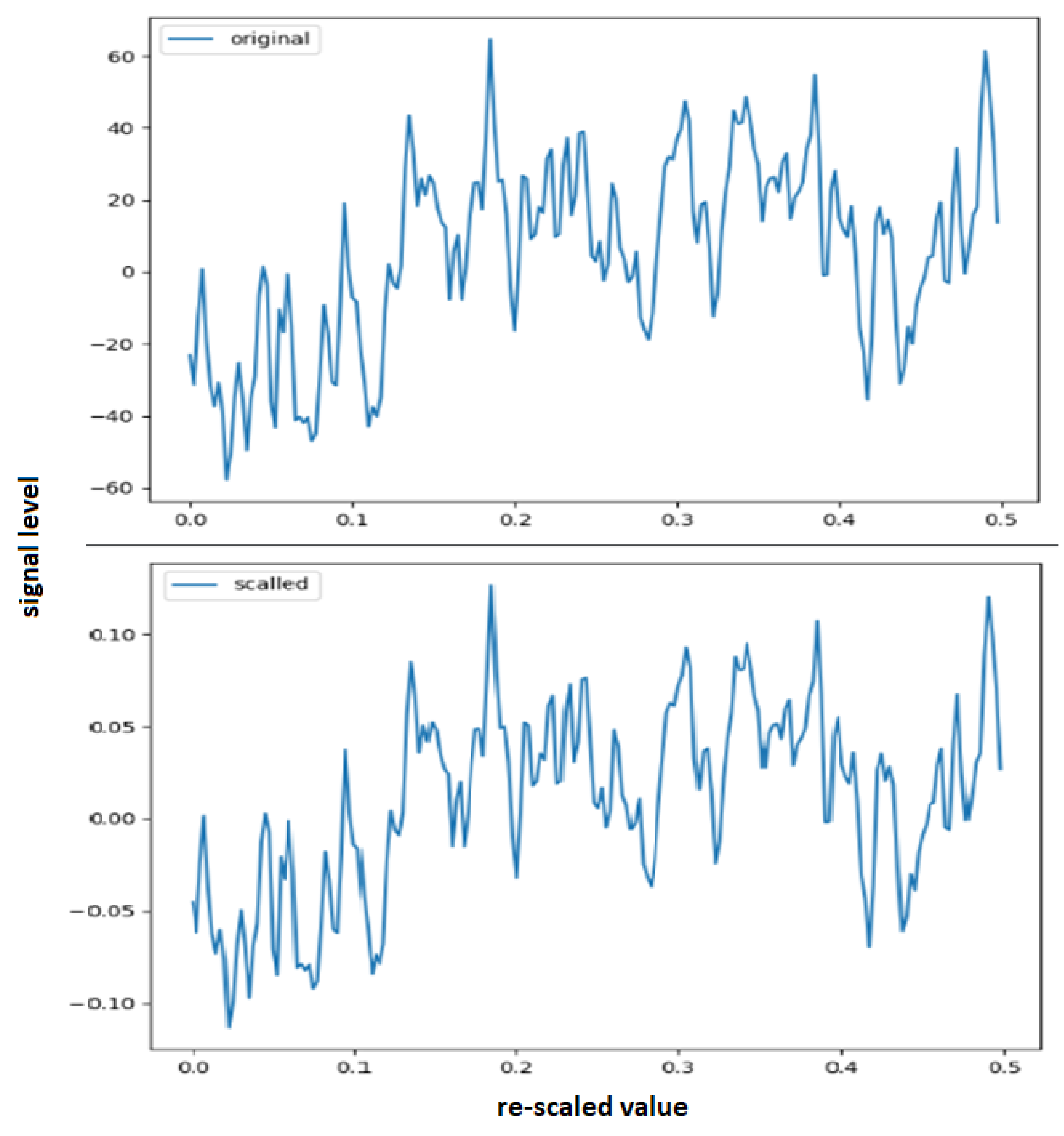
3.3.2. Data Scaling

We tested our model on Sleep EEG datasets with data scaling and without data scaling. We found that the model performed better with data scaling. However, a Recurrent Neural Network (LSTM) tends to learn better with small values, so we scaled the data to between −1 and 1. A sample showing original and rescaled values re-scaled data is seen in Figure 3.

4. Interpretation of Pharmaco-EEG Fingerprint Using Frequency Analysis

During the pre-treatment period, EEG recording was performed for 30 min. Signals collected during the pre-treatment were used to determine the baselines for scaling further data (to % baseline). Then, effects on spectral EEG power were observed for 180 min after treatment with either distilled water, diazepam, or lavender EO. Changes in the recorded electrical power $(V2/Hz)$ were expressed as percent of baseline in 30 min intervals. The spectral powers were then averaged within specific frequency ranges as given in

Table 1. Frequency ranges for computing spectral power.

Delta [$\mathsf{\Delta }$]	Theta [$\mathsf{\Theta }$]	Alpha1 [${\mathit{\alpha }}_1$]	Alpha2 [${\mathit{\alpha }}_2$]	Beta1 [${\mathit{\beta }}_1$]	Gamma [$\mathsf{\Gamma }$]
0.78–4.30	4.69–6.64	7.03–9.38	9.77–12.50	12.89–18.36	35.55–45.31

, and Pharmaco-EEG fingerprint was plotted as a color-coded graph.

Visual inspection was done to overview the recorded EEG signals. To remove the noise from power line artefacts, 50 Hz notch filtering was used: the signals of 45–55 Hz were excluded from further analysis.

The digitized data were subjected to frequency analysis, which included power spectral density (PSD) and spectrogram analysis (frequency versus time plots). The signals were transformed to power spectra using the FFT, after the EEG data were divided into 1024-point bins with 50% overlap (Hanning window cosine transform, 2.56-s sweeps per window, 0.39 Hz frequency resolution).

5. Sleep Stages of Rodents

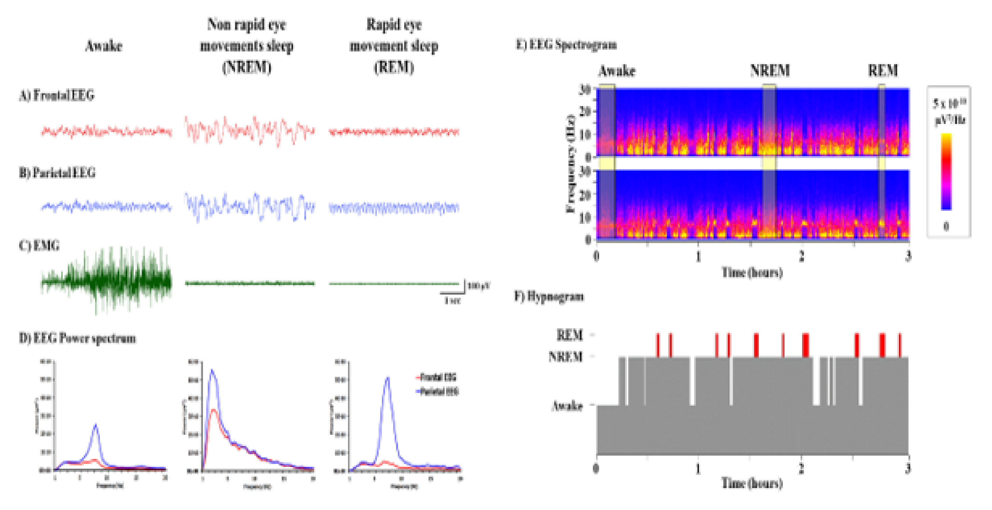
Visual inspection of the EEG and EMG patterns separated the basic states of sleep-wake profiles, which included awake, non-rapid eye movements sleep (NREM), and rapid eye movements sleep (REM); see Figure 4. Based on earlier research, EEG and EMG patterns were used to rate sleep-wake states.

Awake: the period was determined by the frontal signal’s fast wave and low amplitude, as well as the presence of high EMG activity. Slow wave and high amplitude frontal and parietal signals were used to identify NREM sleep stage. Fast wave and low amplitude of the frontal signal, as well as the absence of EMG activity, were used to detect REM: sleep. Theta frequency (Hz) amplitude in the parietal cortex was found to be a key feature of REM sleep.

Between the three stages, EEG power spectra from both the frontal and parietal cortices show distinguishing patterns (Figure 4). The sleep-wake cycles were also validated visually with the help of a spectrogram. It was easy to distinguish the phases of Wake, NREM, and REM sleep using representative colors of EEG power. As a result, the length of each segment was measured in order to produce a hypnogram. For statistical analysis, each variable in each group was averaged.

6. Long-Short-Term Memory Neural Network (LSTM)

RNN is among the popular neural networks used with sequence data. An RNN comprises several hidden layers distributed across the previous time-steps. Such sequence models are capable of storing previous information to predict a future output [18]. Due to the sequence inputs, RNNs are considered computationally very complex and intensive models.

In their applications within different domains, such models have not been able to handle long-term dependencies due to forgetting the long-term effects in back-propagation of current error [19]. This limitation of RNN is called ’the vanishing gradient problem’. This vanishing gradient problem occurs due to lack of ($h_{t-1}$) in Equation (1), where the long-term effects of derivatives of $h_{t-1}$ with respect to $h_t$ vanish. Here, $x_t$, $h_t$, and $y_t$ represent input, hidden state, and output at time step t. Moreover, tanh and sigmoid activation functions are applied for nonlinearity:

$$\left\{\begin{array}{c}{h}_t=tanh(W_h{x}_t+w_{hy}{y}_{t-1})\\ y_t=\sigma \left(W{h}_t\right)\end{array}\right\}$$

(1)

In order to cope with this challenge, we have employed an updated version of RNN widely known as LSTM. It includes an additional and complex block of components, called gates, which store the necessary information from previous time-steps [19,20]. These gates significantly eliminate the vanishing gradient problem by including long-term gradient dependencies.

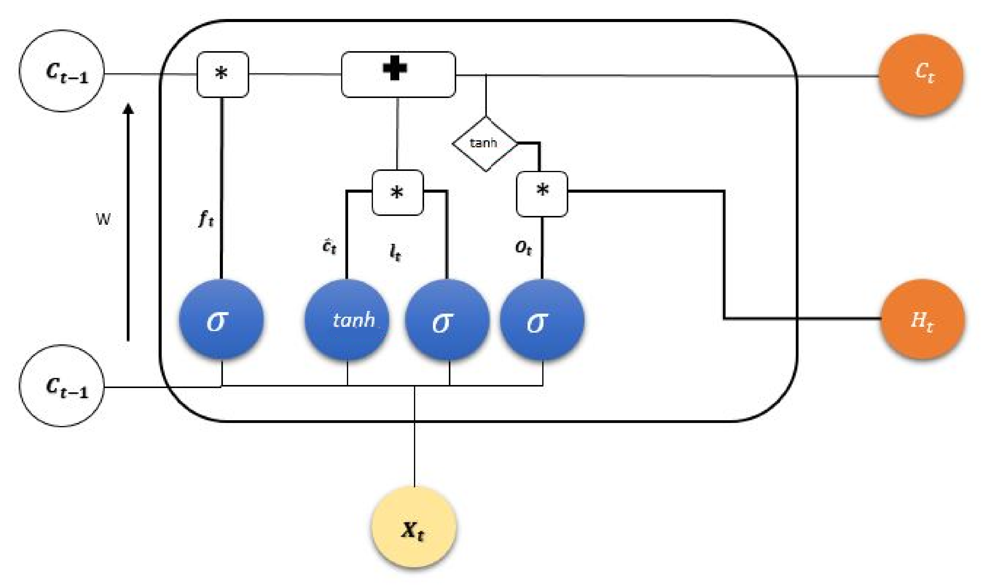
Recently, LSTM has gained remarkable attention in scientific communities associated with different domains [21]. In addition to the explicit memory element, the model comprises an input, output, and forget gate. Each gate in the cell (see Figure 5) receives inputs from preceding time-steps such as $x_t$ and $h_{t-1}$ as inputs from current state and from the hidden states, respectively. Moreover, the state information $C_{t-1}$ is in the cell’s internal memory to retain the necessary information from preceding time-steps. The output at time-step t1 is determined by applying the tanh activation function at the hidden unit of the previous time-step, i.e., $h_{t-1}$. This provides nonlinearity to the model, which significantly improves learning capabilities of the LSTM architecture.

The overall processing of one time-step in LSTM is described as follows: Unnecessary information from previous time-steps is rectified by applying sigmoid activation function, which is termed the forget gate and mathematically defined as

$$f\left(t\right)=\sigma \left[w{W}_f(h_{t-1},x_t)+b_f\right]$$

(2)

Here, $W_f$ is a weight matrix and $h_{(t-1)}$ is the output from previous time-step, $x_t$ is the updated input, and $b_f$ is the bias term.

Furthermore, the information to be stored in the cell memory is determined by a sigmoid activation function often called an input gate in LSTM literature. Then, the tanh layer produces a vector, which is represented by $\widehat{c}$ It could be further added to the state as follows:

$$\left\{\begin{array}{c}{i}_t=\sigma \left[w_i(h_{t-1},x_t)+b_i\right]\\ {\widehat{c}}_i=tanh\left[W_c(h_{t-1},x_t)+b_i\right]\end{array}\right\}$$

(3)

On the basis of candidate state, the old cell state is updated with new cell state as follows:

$$c_t=f_t\ast c_{t-1}+i_t\ast {\widehat{c}}_t$$

(4)

Finally, the output of cell state is passed through a sigmoid activation function which uses part of the information, from a previous stage:

$$o_t=\sigma \left[W_o(h_{t-1},x_t)+b_i\right]$$

(5)

$$h_t=o_t\ast tanh\left(c_t\right)$$

(6)

In this study, we exploited the capabilities of the LSTM architecture shown in

Table 2. Summary of the RNN model.

Layer (Type)	Output Shape	No. of Params
lstm (LSTM)	(None, 100, 55)	12,760
dropout (Dropout)	(None, 100, 55)	0
$lst{m}_1$ (LSTM)	(None, 100, 100)	62,400
$dropou{t}_1$ (Dropout)	(None, 100, 100)	0
$lst{m}_2$ (LSTM)	(None, 40)	22,560
$dropou{t}_2$ (Dropout)	(None, 40)	0
dense (Dense)	(None, 100)	4100
$dropou{t}_3$ (Dropout)	(None, 100)	0
$dens{e}_1$ (Dense)	(None, 3)	303

. In addition to this, we have addressed potential over fitting by employing two regularization techniques, namely by including dropout with 0.2 probability at the dropout layer, and, secondly, by using the learning rate 0.0003 to avoid overshoot problem in the gradient.

7. LSTM Architecture

We have tested two different approaches, namely RNN (LSTM) and hybrid approach (LSTM and 1DCNN). We found that RNN (LSTM) performed better. However, in this study, we present an improved approach, namely LSTM that includes a “memory cell” capable of storing information for lengthy periods of time. Our LSTM is based on the following configuration: For each EEG window, the number of data points in one-time series is 100, and the number of features is 2 or 1.

However, in the first LSTM layer, we have 12,760 parameters, and the output size is 55 with 100 data points. The second LSTM1 layer has 62,400 parameters, and its output size is 100 with 100 data points. The third LSTM2 layer has 22,560 parameters, and the output size is 40.

Two dense layers were added to the model. The first dense layer D1 was used after the LSTM2 layer and its output size is (4100, 100). The second dense layer D2 is used as the last one, with output size (303, 3). Moreover, to deal with the over fitting problem, we utilized two regularization techniques, one of which is dropout with 0.2 probability in the dropout layer. Secondly, the learning rate 0.0003 was used to fix the gradient problem in the model. A complete summary of our RNN model is given in Table 2.

8. Experimental Results

In this section, the results from the experimentation are presented and elaborated.

8.1. Performance Evaluation of Electrode Positions

A number of performance metrics of a classifier were employed, and precision of the model developed is assessed in the results presented.

8.1.1. Classification Accuracy

Precision, recall, F1-score, and support describe the performance of the model in each class label [22]. Precision indicates the number of true positives and the number of false negatives in each class label. However, precision is typically used along with recall metrics to define the ratio of positive instances correctly classified by the model. F1-score indicates the combination of both precision and recall, and support defines the event of each class that lies in a targeted class. For binary and multiclass classifications,

Table 3. Performance measures for binary and multiclass classifications.

SINGLE PC ELECTRODE
NREM and REM
Classification Problem	Stages	Precision	Recall	F1-Score	Support
BINARY	NREM	0.92	0.99	0.96	46,138
	REM	0.60	0.14	0.22	4360
	Accuracy	0.92
	NREM and Wake
	NREM	0.82	0.90	0.86	46,312
	WAKE	0.75	0.60	0.67	23,374
	Accuracy	0.80
	Wake and REM
	WAKE	0.87	0.98	0.92	23,455
	REM	0.64	0.22	0.32	4344
	Accuracy	0.86
NREM, REM, Wake
MULTI CLASS	NREM	0.80	0.88	0.84	46,158
	REM	0.61	0.23	0.33	4362
	WAKE	0.72	0.66	0.69	23,471
	Accuracy	0.77

,

Table 4. Performance measures for binary and multiclass classifications.

SINGLE FC ELECTRODE
NREM and REM
Classification Problem	Stages	Precision	Recall	F1-Score	Support
BINARY	NREM	0.92	1.00	0.96	46,255
	REM	0.74	0.08	0.14	4243
	Accuracy	0.92
	NREM and Wake
	NREM	0.85	0.91	0.88	46,239
	WAKE	0.85	0.91	0.88	23,447
	Accuracy	0.83
	Wake and REM
	WAKE	0.86	0.99	0.92	23,552
	REM	0.63	0.12	0.21	4247
	Accuracy	0.85
NREM, REM, Wake
MULTI CLASS	NREM	0.82	0.91	0.86	46,230
	REM	0.55	0.14	0.23	4307
	WAKE	0.74	0.69	0.71	23,454
	Accuracy	0.79

and

Table 5. Performance measures for binary and multiclass classifications.

SINGLE PC-FC ELECTRODE
NREM and REM
Classification Problem	Stages	Precision	Recall	F1-Score	Support
BINARY	NREM	0.94	0.99	0.96	46,073
	REM	0.69	0.35	0.46	4425
	Accuracy	0.93
	NREM and Wake
	NREM	0.85	0.91	0.88	46,181
	WAKE	0.80	0.68	0.73	23,505
	Accuracy	0.83
	Wake and REM
	WAKE	0.88	0.98	0.93	23,515
	REM	0.70	0.29	0.41	4284
	Accuracy	0.87
NREM, REM, Wake
MULTI CLASS	NREM	0.86	0.89	0.88	46,368
	REM	0.68	0.36	0.47	4297
	WAKE	0.75	0.76	0.75	23,326
	Accuracy	0.82

provide precision, recall, F1-scores, and support metrics. The model’s precision is lowest for the REM stage, and this, together with the similar recall score for REM, indicates that the classifier is unable to learn to recognize the REM stage. In its predictions, it is unable to precisely categorize every actual occurrence of REM. The NREM and Wake stages were predicted more accurately than the REM state. This may be due to the fact that they have a greater number count in the training data.

It is apparent from the table that the accuracy of binary classification was 92% when NREM and REM stages were combined. It is surprising that, when a class with a large number of occurrences is combined with others, the classifier accuracy increased to 92%. Interestingly, the class imbalance affects the classification performance. It can apply a key effect on significance and accuracy, and on other performance metrics [23].

Multiclass classification accuracy is lower than that of binary classification as shown in Table 3. The data complexity is increased with the addition of more classes. It is observed that the classification performance is affected negatively whether the data are balanced or not. We conclude that the multiclass problem cannot be simply solved by adding more classes.

8.1.2. Training and Validation Loss

Table 6. Validation loss and accuracy for a single PC electrode.

NREM AND REM
NREM AND WAKE
WAKE AND REM
NREM, REM, WAKE

,

Table 7. Validation loss and accuracy for a single FC electrode.

NREM AND REM
NREM AND WAKE
WAKE AND REM
NREM, REM, WAKE

and

Table 8. Validation loss and accuracy for a single PC-FC electrode.

NREM AND REM
NREM AND WAKE
WAKE AND REM
NREM, REM, WAKE

show the validation loss and accuracy for binary and multi-class classifications. When REM stages are combined to create a binary classification job, the validation accuracy can be observed to be highly unstable. The fluctuation in validation accuracy can be explained by the fact that the model is still learning the appropriate weights to generalize effectively in validation data. In addition, the fluctuation in validation loss is consistent, which could be due to the initialization of pre-trained weights. In the case of multi-class classification, the validation loss does not appear to be locked in a local minimum and converges smoothly. The validation loss and accuracy have improved.

8.1.3. Confusion Matrix

The confusion matrix, see

Table 9. Confusion matrices.

SINGLE PC ELECTRODE
Predicted
Actual	Stages	NREM	REM
	NREM	47,747	391
	REM	3769	591
	Stages	NREM	WAKE
	NREM	41,720	4592
	Wake	9354	14,020
	Stages	WAKE	REM
	WAKE	22,939	516
	REM	3409	935
	Stages	NREM	REM	Wake
	NREM	40,157	496	5531
	REM	2457	1129	694
	WAKE	7086	286	16,155
Confusion Matrix of Single PC Electrode
SINGLE FC ELECTRODE
Predicted
Actual	Stages	NREM	REM
	NREM	46,144	111
	REM	3923	320
	Stages	NREM	WAKE
	NREM	42,073	4166
	Wake	7593	15,854
	Stages	WAKE	REM
	WAKE	23,246	306
	REM	3726	521
	Stages	NREM	REM	Wake
	NREM	42,095	146	3877
	REM	2020	605	1781
	WAKE	7145	177	16,145
Confusion Matrix of Single FC Electrode
SINGLE PC-FC ELECTRODE
Predicted
Actual	Stages	NREM	REM
	NREM	45,387	686
	REM	2889	1536
	Stages	NREM	WAKE
	NREM	42,154	4027
	Wake	7559	15,946
	Stages	WAKE	REM
	WAKE	22,986	529
	REM	3025	1259
	Stages	NREM	REM	Wake
	NREM	42,124	375	3814
	REM	1508	1654	1198
	WAKE	6029	428	16,861
Confusion Matrix of Single PC-FC Electrode

, shows that the NREM stage is the most accurately classified, followed by Wake and REM stages. In binary classification, the NREM has been mis-classified the most by calling it Wake stage; one explanation could be the increased number of Wake stage cases. In the case of multi-class classification, the most mis-classified stage is Wake mislabeled as NREM.

9. Discussion

We introduced a deep learning based Recurrent Neural Network (RNN) that calls the different states of consciousness in rats from EEG and EMG recordings. The proposed model automatically learns features which exist in the data and uses them to classify sleep stages. We analyzed the challenge of class imbalance problem and investigated the generalization of the model. Two types of class imbalance problems, i.e., minority and majority cases for binary and multiclass classification, were studied in depth. Both types show negative correlations with the performance measures: precision, recall, or F1-Score. This indicates that the performance is inversely proportional to the number of imbalanced classes. The performance trend indicates that performance degraded as the majority group increases. The reason is that the imbalance rate increases in the minority cases.

Based on the analysis, we investigated a dichotomy of the sleep stages, i.e., binary classification with the aim of handling majority and minority classes. When minority and majority class difference was small, the results for Recall and F1-Score improved. This shows that we can do generalization for a minority class, and, furthermore, help to balance performance.

Moreover, the results show that the class decomposition into binary form does not provide any advantages in learning with class imbalance. In the case of REM stage, the Recall and F1-Score were reduced by class decomposition. A possible explanation for this behavior is that the global information of class distribution is reduced as a result of class decomposition. We conclude that a non-decomposition method is better than decomposition because the class distribution information is fully utilized. Hence, the model performance is improved.

Our model achieves high F1 scores in the multi-class problem. Decreasing the number of input channels that were available for our model to infer sleep stages decreased the prediction performance. This shows that our model will yield good prediction performance even for experiments in which multiple channels are included.

For multiple channels and classes, F1 scores became better. This observation agrees with our expectation that the accuracy increases if all channel recordings are available. The prediction performance of our model was poorer for a single channel when compared to multiple channel data. This may, however, be related to our training set, which had many artifact contaminated epochs.

The performance comparison with existing state-of-the-art methods is shown in the following

Table 10. Performance comparison with existing state-of-the-art methods.

Model	Sleep Stages	Accuracy—F1 Score	Reference
Hybrid Model (CNN and LSTM)	Wake, REM and NREM	96.6%	[17]
CNN	Wake, Pre REM, NREM, REM and Artifact	95.0%	[15]
CNN and Radmon Forest	Sleep-wake states	77.0–83.0%	[16]
ANN	Wake, REM and NREM	96.8%	[18]
Proposed method LSTM	Binary classes (Wake-REM, Wake-NREM, REM-NREM), multiple classes (Wake-REM-NREM) with single and multiple electrode position	92.0–79.0%, 93.0–82.0%

. In contrast to those prior studies, the contributions in this study are demonstrating a trainable LSTM network model, along with addressing the following questions: how effective are single and alternatively multiple electrode positions for rodent sleep stage classification, and is binary or multiclass classification more effective?

We are interested in sleep stage combinations, seeking better balance, and their effect on classifier performance. As each electrode has its position in signal recording, it is important to appreciate that sleep scoring performance is sensitive to the position(s) of a single or of multiple electrodes. Furthermore, a classification algorithm is hampered by the unbalance when one class with only few instances co-exists with another class of a much larger size, in the training data.

10. Conclusions

The proposed RNN and LSTM method can find automatically effective features that would be difficult to extract using handcrafted filters. The experimental results reveal that the classification accuracy is affected by the selection of multiple electrode positions as well as by the classification problem posed. In the multi-class problem, imbalance appears challenging, while binary-class imbalance can be less, but still, in the case of multiple electrode positions, a high accuracy was achieved for multiple classes. In future research, we may pursue finding optimal hyper-parameters for training a classifier; this is another important and interesting topic.

References

- Toth, L.A.; Bhargava, P. Animal models of sleep disorders. Comp. Med. 2013, 63, 91–104. [Google Scholar] [PubMed]
- Pagel, J.; Parnes, B.L. Medications for the treatment of sleep disorders: An overview. Prim. Care Companion J. Clin. Psychiatry 2001, 3, 118. [Google Scholar] [CrossRef] [PubMed]
- Oishi, Y.; Takata, Y.; Taguchi, Y.; Kohtoh, S.; Urade, Y.; Lazarus, M. Polygraphic recording procedure for measuring sleep in mice. JoVE (J. Vis. Exp.) 2016, 107, e53678. [Google Scholar] [CrossRef] [PubMed] [Green Version]
- Kadam, S.D.; D’Ambrosio, R.; Duveau, V.; Roucard, C.; Garcia-Cairasco, N.; Ikeda, A.; de Curtis, M.; Galanopoulou, A.S.; Kelly, K.M. Methodological standards and interpretation of video-EEG in adult control rodents. A TASK1-WG1 report of the AES/ILAE Translational Task Force of the ILAE. Epilepsia 2017, 58, 10. [Google Scholar] [CrossRef] [PubMed] [Green Version]
- Davis, E.M.; O’Donnell, C.P. Rodent models of sleep apnea. Respir. Physiol. Neurobiol. 2013, 188, 355–361. [Google Scholar] [CrossRef] [PubMed] [Green Version]
- Schwabedal, J.T.; Sippel, D.; Brandt, M.D.; Bialonski, S. Automated classification of sleep stages and EEG artifacts in mice with deep learning. arXiv 2018, arXiv:1809.08443. [Google Scholar]
- Altevogt, B.M.; Colten, H.R. Sleep Disorders and Sleep Deprivation: An Unmet Public Health Problem; National Academies Press (US): Washington, DC, USA, 2006. [Google Scholar]
- Manaswi, N.K. Rnn and lstm. In Deep Learning with Applications Using Python; Springer: Berlin/Heidelberg, Germany, 2018; pp. 115–126. [Google Scholar]
- Bastianini, S.; Berteotti, C.; Gabrielli, A.; Martire, V.L.; Silvani, A.; Zoccoli, G. Recent developments in automatic scoring of rodent sleep. Arch. Ital. De Biol. 2015, 153, 58–66. [Google Scholar]
- Sunagawa, G.A.; Sei, H.; Shimba, S.; Urade, Y.; Ueda, H.R. FASTER: An unsupervised fully automated sleep staging method for mice. Genes Cells 2013, 18, 502–518. [Google Scholar] [CrossRef] [PubMed] [Green Version]
- Suzuki, Y.; Sato, M.; Shiokawa, H.; Yanagisawa, M.; Kitagawa, H. MASC: Automatic sleep stage classification based on brain and myoelectric signals. In Proceedings of the 2017 IEEE 33rd International Conference on Data Engineering (ICDE), San Diego, CA, USA, 19–22 April 2017; pp. 1489–1496. [Google Scholar]
- Gao, V.; Turek, F.; Vitaterna, M. Multiple classifier systems for automatic sleep scoring in mice. J. Neurosci. Methods 2016, 264, 33–39. [Google Scholar] [CrossRef] [PubMed] [Green Version]
- Yaghouby, F.; O Hara, B.F.; Sunderam, S. Unsupervised estimation of mouse sleep scores and dynamics using a graphical model of electrophysiological measurements. Int. J. Neural Syst. 2016, 26, 1650017. [Google Scholar] [CrossRef] [PubMed]
- Yamabe, M.; Horie, K.; Shiokawa, H.; Funato, H.; Yanagisawa, M.; Kitagawa, H. MC-SleepNet: Large-scale sleep stage scoring in mice by deep neural networks. Sci. Rep. 2019, 9, 1–12. [Google Scholar] [CrossRef] [PubMed]
- Svetnik, V.; Wang, T.C.; Xu, Y.; Hansen, B.J.; Fox, S.V. A deep learning approach for automated sleep-wake scoring in pre-clinical animal models. J. Neurosci. Methods 2020, 337, 108668. [Google Scholar] [CrossRef] [PubMed]
- Barger, Z.; Frye, C.G.; Liu, D.; Dan, Y.; Bouchard, K.E. Robust, automated sleep scoring by a compact neural network with distributional shift correction. PLoS ONE 2019, 14, e0224642. [Google Scholar] [CrossRef] [PubMed]
- Grieger, N.; Schwabedal, J.T.; Wendel, S.; Ritze, Y.; Bialonski, S. Automated scoring of pre-REM sleep in mice with deep learning. Sci. Rep. 2021, 11, 1–14. [Google Scholar] [CrossRef] [PubMed]
- Elsaraiti, M.; Merabet, A. Application of Long-Short-Term-Memory Recurrent Neural Networks to Forecast Wind Speed. Appl. Sci. 2021, 11, 2387. [Google Scholar] [CrossRef]
- Zhao, Z.; Chen, W.; Wu, X.; Chen, P.C.; Liu, J. LSTM network: A deep learning approach for short-term traffic forecast. IET Intell. Transp. Syst. 2017, 11, 68–75. [Google Scholar] [CrossRef] [Green Version]
- Bukhari, A.H.; Raja, M.A.Z.; Sulaiman, M.; Islam, S.; Shoaib, M.; Kumam, P. Fractional neuro-sequential ARFIMA-LSTM for financial market forecasting. IEEE Access 2020, 8, 71326–71338. [Google Scholar] [CrossRef]
- e Gonçalves, W.G.; Dos Santos, M.H.d.P.; Lobato, F.M.F.; Ribeiro-dos Santos, Â.; de Araújo, G.S. Deep learning in gastric tissue diseases: A systematic review. BMJ Open Gastroenterol. 2020, 7, e000371. [Google Scholar] [CrossRef] [PubMed] [Green Version]
- Geron, A. Hands-On Machine Learning with Scikit-Learn & Tensorflow O’Reilly Media, Inc.; O’Reilly Media, Inc.: Sebastopol, CA, USA, 2017; p. 564. [Google Scholar]
- Luque, A.; Carrasco, A.; Martín, A.; de Las Heras, A. The impact of class imbalance in classification performance metrics based on the binary confusion matrix. Pattern Recognit. 2019, 91, 216–231. [Google Scholar] [CrossRef]