Model Test Study of Offshore Wind Turbine Foundation under the Combined Action of Wind Wave and Current

Abstract

The wind turbine system in the offshore area will be subjected to the combined action of complex marine environment dynamic loads. At present, there is a certain advantage to using traditional mechanical devices to simulate marine environmental loads. In this study, the self-developed complex dynamic load test loading system is adopted to carry out a series of model tests for pile foundations. The theoretical calculation results of wind, wave and current load are applied to the wind turbine system, and the responses of the pile and soil are analyzed according to the actual model test. The main conclusions are as follows: the development of pile displacement is basically linear with the logarithm of cycle times, and pile–soil interaction is directly affected by the form of load, the results of dynamic response obtained in this test are closer to that under the actual marine environmental load.

1. Introduction

With the vigorous promotion of carbon neutrality in various countries, offshore wind energy, as a representative of clean and renewable energy, plays a role in improving the energy structure of various countries. As an important component bearing the dead weight of the upper wind turbine structure and external complex marine environmental loads, the foundation of offshore wind turbines has complex interactions with the seabed. Generally speaking, the vertical bearing performance of the pile foundation can meet the requirements, while the horizontal load has a great influence on the safety of the pile foundation structure (2021) [1]. The research took horizontal and vertical amplitude and frequency of motion of input structure as variables to study the effect of earthquakes on settlement of end-bearing piles. The results showed that earthquakes will cause more severe liquefaction of sand layers with distant structures, thus causing greater settlement of group piles. In addition, under the action of extreme wind, wave and current loads, the pore water pressure in the seabed around the pile may increase, which in turn leads to a decrease in the bearing capacity of the seabed and even seabed liquefaction (2021) [2]. In this study, a complete three-dimensional numerical model was established to consider the frequency domain characteristics of a single pile seawater–seabed coupling system, and the dynamic interaction between pile body, seabed and seawater was fully considered. The transient liquefaction occurred in the area near two-thirds of the diameter of the pile. Under the action of long-term wind, wave and current loads, the foundation will have accumulated displacement (2020) [3], and the final wind turbine rotation angle may exceed the design allowable value, resulting in the failure and damage of the wind turbine structure. In this study, the results of a systematic model test study dealing with the response of monopiles to lateral cyclic loading in medium dense sand at different cyclic load ratios, load eccentricities and pile embedment lengths were described and evaluated. Based on the findings and the results, recommendations regarding the prediction of displacement accumulations for large-diameter monopiles in sand were given. Therefore, it has important theoretical significance and engineering practical value to study the dynamic response of wind turbine foundation under the action of wind, wave and current load.

Since experimental research can describe the law of pile–soil interaction more intuitively, many researchers currently use various experimental methods to conduct research on offshore wind turbine foundations under complex ocean loads. For example, field test, wave pool and wind tunnel test, centrifuge test, among which the most widely used is constant gravity model test (2013) [4]. From the perspective of experimental technology, in the current experimental research on offshore wind turbine foundations, prototype observations and field tests can more realistically reflect the effect of original sea conditions on structures. Pan et al. (2016) [5] carried out field tests under vertical and horizontal loads on offshore wind turbine foundations. The study found that the pile–soil interaction is very sensitive to the nonlinear characteristics of the soil and found that the results using the p–y curve method recommended by the API code overestimated the displacement and bending moment of large-diameter piles in clay. Zhu et al. (2012) [6] carried out a series of field tests on large-diameter high-pile foundations in the ocean for soft clay sites and proposed a hyperbolic p–y curve suitable for the test results. At the same time, the method of deriving the displacement, bending moment and soil resistance of the pile body according to the measured data is effective. However, in general, due to the particularity of the original site, such tests are only aimed at sea conditions in some special sea areas, and their applicability is limited. On the other hand, due to the difficulty of offshore operation and the difficult control of test conditions, it is difficult to obtain effective data on the dynamic response of wind turbine pile foundations in such tests.

In addition, the current wave pool and boundary layer wind tunnel test technology provides the possibility to simulate the real marine environment, such as (2014, 2009, 2008) [7,8,9], such projects have developed and installed multiple wave generators that can generate high and multi-directional deep-water waves while allowing stratified surface flow in one direction. With only one correction, the system can accurately generate a new wave field from zero. However, there are also problems such as imperfect wind and wave control technology and low performance of wave and wind generation. At present, there are many experiments on new structural forms such as floating wind turbine foundation, but there are few experiments using such techniques to investigate the interaction of piles and soils.

When the test conditions for wave and wind generation are lacking, most researchers actively design and develop simple mechanical devices to simulate the effect of marine environmental loads on structures. The main method is to simplify the complex marine environmental loads into low-frequency cyclic loads. For example, the Danish scholar Hansen (2012) [10] used the actuator to load by “rocking pile” to simulate the horizontal circulation effect of the dynamic load of the marine environment on the monopile foundation. In addition, most scholars used self-developed loading devices (2012) [11] to load the model structure to meet the loading requirements of high-cycle tests, the realization principle was to use the reciprocating eccentric wheel to drive the pile movement, and this kind of device had been adopted by many famous scholars at home and abroad. However, such loading devices cannot arbitrarily change the load frequency and amplitude in a single test. It is difficult to consider the difference in the directionality of the marine environment load, so the load characteristics of this kind of test load and the real marine environment are also different.

In response to this problem, this study takes an offshore wind turbine project in the Jiangsu sea area of China as the background, and conducts a series of model tests for the offshore wind turbine monopile foundation in the saturated sandy soil foundation. First, select reasonable wind, wave and current calculation parameters in the prototype sea state. Based on the harmonic superposition method and Stokes’ second-order wave theory, the wind load time history, wave and ocean current load time history of the prototype wind turbine were calculated, and the test load is obtained by scaling the prototype load through the dynamic similarity relationship. Then, the powerful servo control system is used to complete the precise control of the wind, wave and current load, and it is applied to the model structure to carry out the test. During the test, the results of dynamic response such as the resistance of soil around the pile, the displacement of the pile body and the pore water pressure of the soil around the pile were obtained, and the law of dynamic response was analyzed.

2. Experimental design

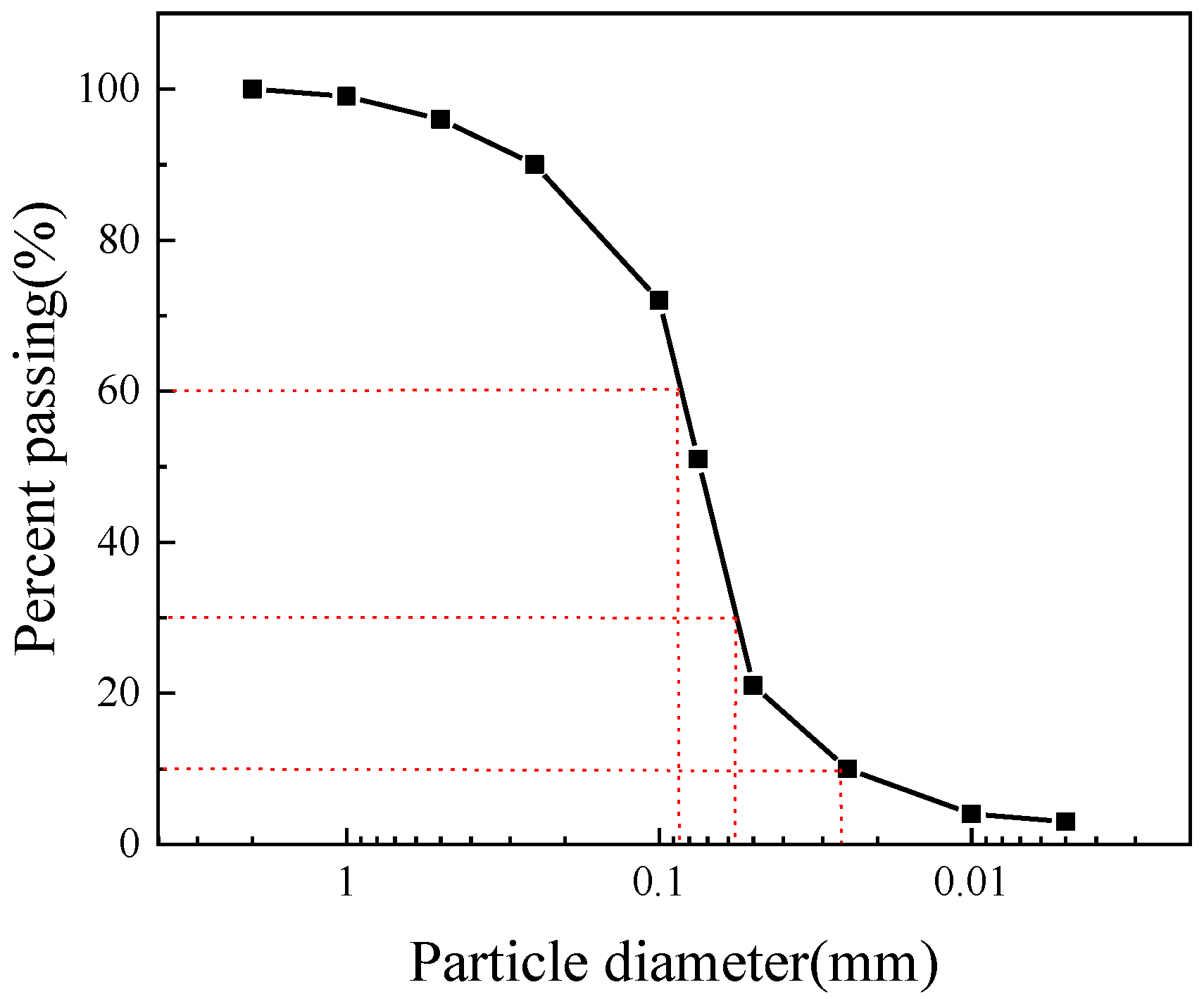
2.1. Test Soil

The series of model tests were carried out in a model box. According to the prototype site conditions, sandy soil samples were used and the foundation was prepared in layers. The thickness of each layer of filling was 10 cm. The relative density of the sandy soil foundation was controlled to be approximately 60% in the test, which was medium-density sandy soil. Calculate the required mass of each layer of fill based on the minimum dry density, and complete the sand saturation during the layered filling process of the foundation. The specific method is as follows: first, fill the soil sample after weighing into the model box, and use a vibrating plate with a vibration frequency of 10 Hz to make the soil sample flat, and the height of the soil sample after vibrating and compacting is 10 cm. After that, water is injected into the box, and the water surface is always kept below the soil surface, and it is allowed to stand for a period of time. During this period, the pore water pressure gauge is used to monitor the hydrostatic pressure value of the place, and wait for the soil layer to be drained. After the indicated numbers are stable, the next layer of soil shall be filled with the same method. In addition, three soils were taken at different positions of each layer of soil samples for density measurement, and the filling of each layer was as uniform as possible, and the final thickness of the filling layer was 1.3 m.

Figure 1 shows the grain-size distributions curve of the sand used in the model test. It can be seen from the figure that the gradation of the sand used in this test is continuous. According to the geotechnical test specification, the measured parameters of the soil sample are as follows: the specific gravity of soil particles is 2.634, the internal friction angle of sandy soil is 35°, the natural void ratio is 0.742, the dry density is 1.510 g·cm⁻³, and the saturated density is 1.936 g·cm⁻³.

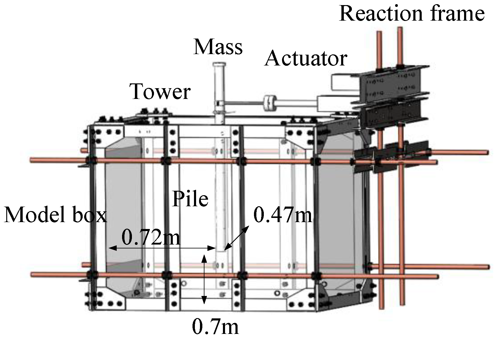
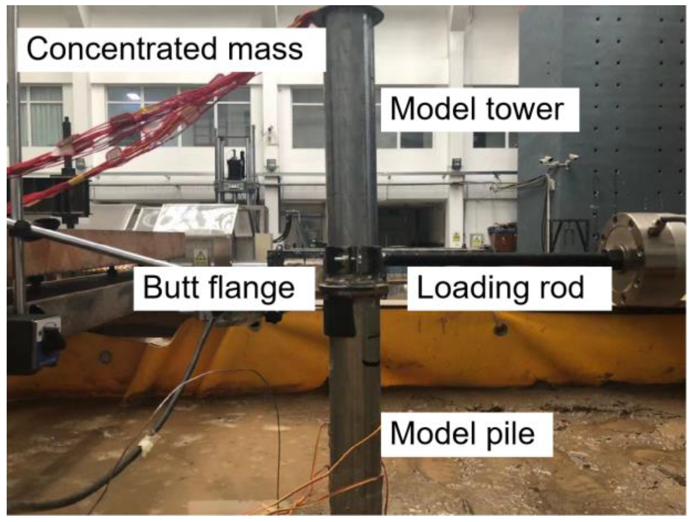
2.2. Model Structure

The model structure design prototype in this series of tests is taken from the actual engineering project data of a wind farm. The parameters of a single pile foundation in the project prototype are as follows: the prototype pile is a large-diameter hollow open steel pipe pile, the diameter of the pile body is 4.20 m, the length of the pile is 63 m, the wall thickness is 70 mm, and the burial depth is 42 m.

According to the steel pipe pile and fan parameters in the actual project data, the model structure of the three important components of the steel pipe pile, the tower and the superstructure was made. In order to make the prototype and model closer, the mass ratio of the three parts was controlled to be consistent. The model pile is made of hollow homogeneous steel pipe. The diameter of the model pile is 0.06 m, the length of the pile is 0.9 m, the wall thickness is 1.2 mm, and the buried depth is 0.6 m. Since the mass ratio of the prototype tower to the steel pipe pile is 1:3, the model tower is made of the same material as the model pile, and the length is simplified to 0.3 m. The steel pipe pile and the tower are bolted by butt flanges. The upper concentrated mass was replaced by an open aluminum plate, which is convenient for the strain gauge wire to pass through the pile and reduces the influence on the soil stress field. The physical diagram of the model structure and the field test diagram are shown in Figure 2.

In order to avoid the disturbance of the soil and the influence of pore pressure caused by piling, a self-made limit device was used to assist the embedding of the model structure, and the pore water pressure gauge was also arranged during the process of burying the pile.

2.3. Similarity Relationship

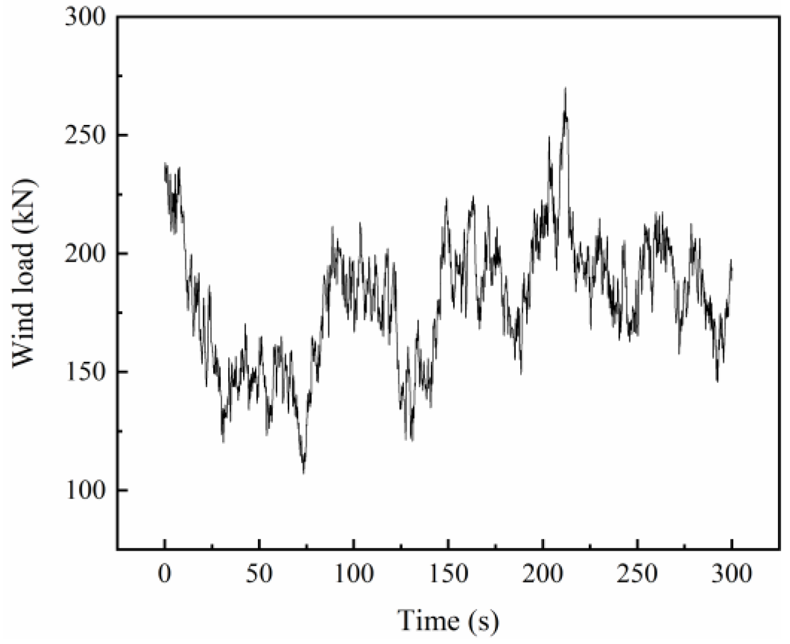
To correlate model test results with prototype responses. Buckingham’s π theorem (1915) [12] was used to deduce and calculate the main physical quantities involved in the test process, which is consistent with the consideration of the similarity relationship in Cuéllar’s test (2012) [13]. The specific similarity relationship of the main physical quantities is shown in

Table 1. Similarity relationship of the main physical quantity.

Physical Quantity	Law of Similarity	Dimension
Length, L	LM = LP/λ	L [m]
Force, F	FM = FP/λ3	F [N]
Uniform line load, q	qM = qP/λ2	F/L [N/m]
Stress, σ	σM = σP/λ	F/L2 [Pa]
Unit weight, γ	γM = γP	F/L3 [N/m3]
Moment, M	MM = MP/λ4	F × L [N·m]
Bending rigidity, EI	(EI)M = (EI)P/λ5	F × L2 [N·m2]
Time, t	tM = tP/λ1/2	T [s]
Frequency, f	fM = fP/λ−1/2	1/T [Hz]

.

In order to ensure that the deformation modes of the prototype structure and the model monopile are consistent, Poulos and Hull’s calculation method of relative pile–soil stiffness was adopted to determine the pile–soil relative stiffness (1989) [14]. According to the definition of the critical depth L_c of the pile foundation, when the depth of the pile foundation is less than one-third of the critical depth, the pile foundation can be regarded as rigid, where L_c is calculated according to the following formula:

$$L_{\mathrm{c}}=4.44(\frac{E_{\mathrm{p}}{I}_{\mathrm{p}}}{E_{\mathrm{s}}}{)}^{0.25}$$

(1)

In the above formula, E_pI_p is the flexural stiffness of the pile body, and E_s is the average elastic modulus of the pile body passing through the soil layer. According to the above formula, the prototype pile and the model pile are calculated, so the relative stiffness of the pile and soil of the model pile in this study is similar to that of the prototype pile, which belongs to the category of semi-rigid piles. Therefore, the deformation modes of the two are considered to be the same.

In addition, due to the limitations of current research methods, the similarity of soil particle size is difficult to fully meet, because the scaling of soil according to the similarity ratio of the above design will lead to significant changes in the properties of sand. However, according to the research conclusions of Ovesen (1979) [15], when the test load is lower than the failure limit and the ratio of foundation diameter to particle size is greater than 30~60, the impact of different particle sizes on the ultimate bearing capacity of the foundation can be ignored. The foundation diameter and particle size in this study meet the above requirements.

2.4. Test Loads

This model test mainly focuses on the dynamic response of wind turbine pile foundation and surrounding seabed under complex marine environmental loads. Therefore, when determining the test load, the wind, wave and current load, which has a more significant impact on the structure among the marine environmental loads, is selected as the design prototype of the test load. In this study, the following load calculation theory is used to simulate the prototype load of the wind turbine.

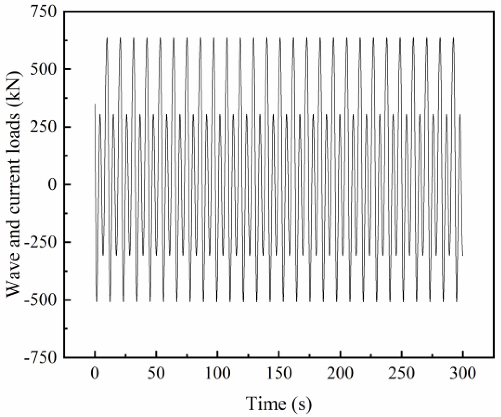
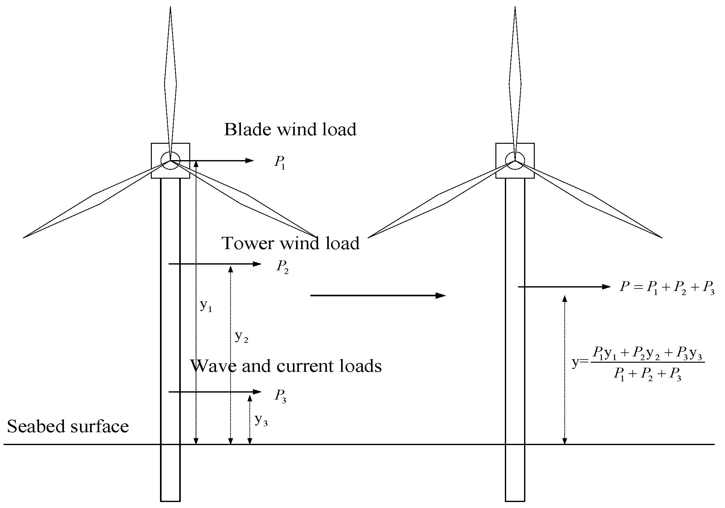
2.4.1. The Calculation Theory of Wind, Wave and Current

Offshore wind turbine systems are subject to complex wind, wave and current loads, in which the sea wind mainly acts on the wind turbine blades and towers, generating huge horizontal thrust and overturning moment on the wind turbine structure and foundation.

In the simulation calculation of wind load, the random natural wind in the real sea state is first decomposed into two parts, the average wind and the pulsating wind, and the exponential wind speed profile with simple form and satisfactory accuracy is used to simulate the characteristics of the average wind along the height. According to the measured parameters of the prototype site, the wind speed at a height of 10 m is taken as 7 m/s. In the wind resistance design code, the exponential formula for simulating the variation of the mean wind speed along the height is as follows:

$$\frac{\overline{u}(z)}{\overline{u}(z_1)}={(\frac{z}{z_1})}^{\alpha }$$

(2)

In the formula, ū(z₁) indicates the average wind speed at the standard height z₁, generally taking z₁ = 10 m; ū(z) indicates the average wind speed at the height z; α is the ground roughness coefficient, and usually α = 0.12 for offshore areas.

The simulation of pulsating wind is completed by the harmonic superposition method with strict algorithm and high precision (2002) [16]. The temporal and spatial variation of pulsating wind speed is usually described by the pulsating wind speed power spectrum and coherence function. In this simulation, the pulsating wind speed power spectrum adopts Simiu spectrum (1970) [17], and the coherence function adopts the Davenport correlation function (1983) [18]. The meanings of formulas and parameters are as follows:

$$S(f)=4k\overline{u}{(10)}^2\frac{x}{f{(1+x^2)}^{4/3}},x=\frac{1200f}{\overline{u}(10)}$$

(3)

$$Coh(r,\omega )=\exp (-\frac{\omega \sqrt{C_x^2{(x_i-x_j)}^2+C_y^2{(y_i-y_j)}^2+C_z^2{(z_i-z_j)}^2}}{2\pi V(z_i)})$$

(4)

In Formula (3), S(f) indicates the power spectrum of pulsating wind speed; f indicates the frequency of pulsating wind; z is the height of any point; x is the similarity law coordinate, which is related to frequency and height; k is the coefficient related to ground roughness, for the offshore sea surface, k = 0.003; ū(10) indicates the average wind speed at a height of 10 m.

In Formula (4), r is the distance between any two points in space; C_x, C_y and C_z are the attenuation coefficients of any two points in space in the lateral, downwind, and vertical directions, which can be taken as 16, 8 and 10, respectively. For a single fan structure, the lateral influence can be ignored, thus C_x = 0; if only the coherence function of each point of the blade or the tower itself is considered, that is, only the vertical coherence is considered, C_x = 0, C_y = 0.

Based on the above calculation principle of wind load, the calculation programs for simulating average wind speed and fluctuating wind speed were compiled by the mathematical calculation software Matlab. By superimposing the above-mentioned average wind speed and pulsating wind speed, the wind speed time history at any time and height within the height range of the wind turbine above sea level can be obtained. For the tower wind load, the wind section of the tower section is divided into 7 blocks, and the wind speed time history of the center point of each small block of the wind plane is simulated as the average wind speed of the wind plane. For blade wind load, the swept area of the blade is taken as the wind receiving area, and then the wind pressure is calculated using the surface load wind pressure calculation formula. Then, the wind load time history at different heights can be obtained by using the blade wind force calculation formula and the artificially divided tower segment action area. Figure 3 shows the simulated wind load time history at the fan hub, that is, the blade wind load. The calculation results of the tower section wind load are similar, but the magnitude of the load is much smaller than the blade wind load.

The effect of waves on small-scale hydraulic structures is generally calculated by the Morison equation. However, there is a complex interaction between currents and waves in the actual marine environment. The existence of ocean current will affect the wave parameters and then the wave force, so the influence of the current velocity is considered in the wave force calculation. The velocity and acceleration of the wave water point are calculated by Stokes’ second-order wave theory and potential wave theory (2018) [19] and the results are put into the Morison equation to obtain the wave force on the pile foundation per unit length. The specific calculation process is as follows:

The ocean current velocity term is introduced into the calculation of the drag force, and the drag force is calculated according to the following formula:

$$f_D=\frac{1}{2}{C}_D\rho D(u_x+u_c)\left|(u_x+u_c)\right|$$

(5)

For a cylinder, the inertial force acting on the pile can be calculated by formula:

$$f_I=C_M\rho \frac{\pi D^2}{4}\frac{\partial u_x}{\partial t}$$

(6)

The horizontal wave force acting on the unit column height at any position z of the upright column is:

$$f_H=f_D+f_I=\frac{1}{2}{C}_D\rho D(u_x+u_c)\left|(u_x+u_c)\right|+C_M\rho \frac{\pi D^2}{4}\frac{\partial u_x}{\partial t}$$

(7)

In the formula, f_D is the drag force; f_I is the inertial force; D is the diameter of the cylinder; ρ is the seawater density; C_D is the drag force coefficient; C_M is the inertial force coefficient; u_x is the horizontal velocity of wave water quality point; u_c is the current velocity. In addition, C_D and C_M can usually be obtained from model tests and field observations. Due to the differences in sea conditions in different countries, the results have great dispersion. According to the load conditions of this study and referring to the marine engineering code, thus C_D = 1.2, C_M = 2.0.

The velocity and acceleration of water quality point motion can be obtained by performing partial differential processing on the velocity potential function. The formulas are expressed as follows:

$$u_x=\frac{\partial {\varphi }_V}{\partial x}=\frac{\pi H_V}{T}\frac{\cosh kz}{\sinh kd}\cos (kx-\omega t)+\frac{3}{4}\frac{{(\pi H_V)}^2}{L_{V}T}\frac{\cosh 2kz}{{\sinh }^{4}kd}\cos 2(kx-\omega t)$$

(8)

$$\frac{\partial u_x}{\partial t}=\frac{2{\pi }^2{H}_V}{T^2}\frac{\cosh kz}{\sinh kd}\sin (kx-\omega t)+3\pi \frac{{(\pi H_V)}^2}{L_V{T}^2}\frac{\cosh 2kz}{{\sinh }^{4}kd}\sin 2(kx-\omega t)$$

(9)

According to the actual wave parameters, the water depth in this test is 5 m, the current velocity is 0.88 m/s, the wave height is 2.13 m, and the wave period is 10.86 s. According to the scope of application of the wave theory proposed by Méhauté (1968) [20], it satisfies the conditions for the use of Stokes’ second-order waves. The calculation results of wave and current loads are shown in Figure 4.

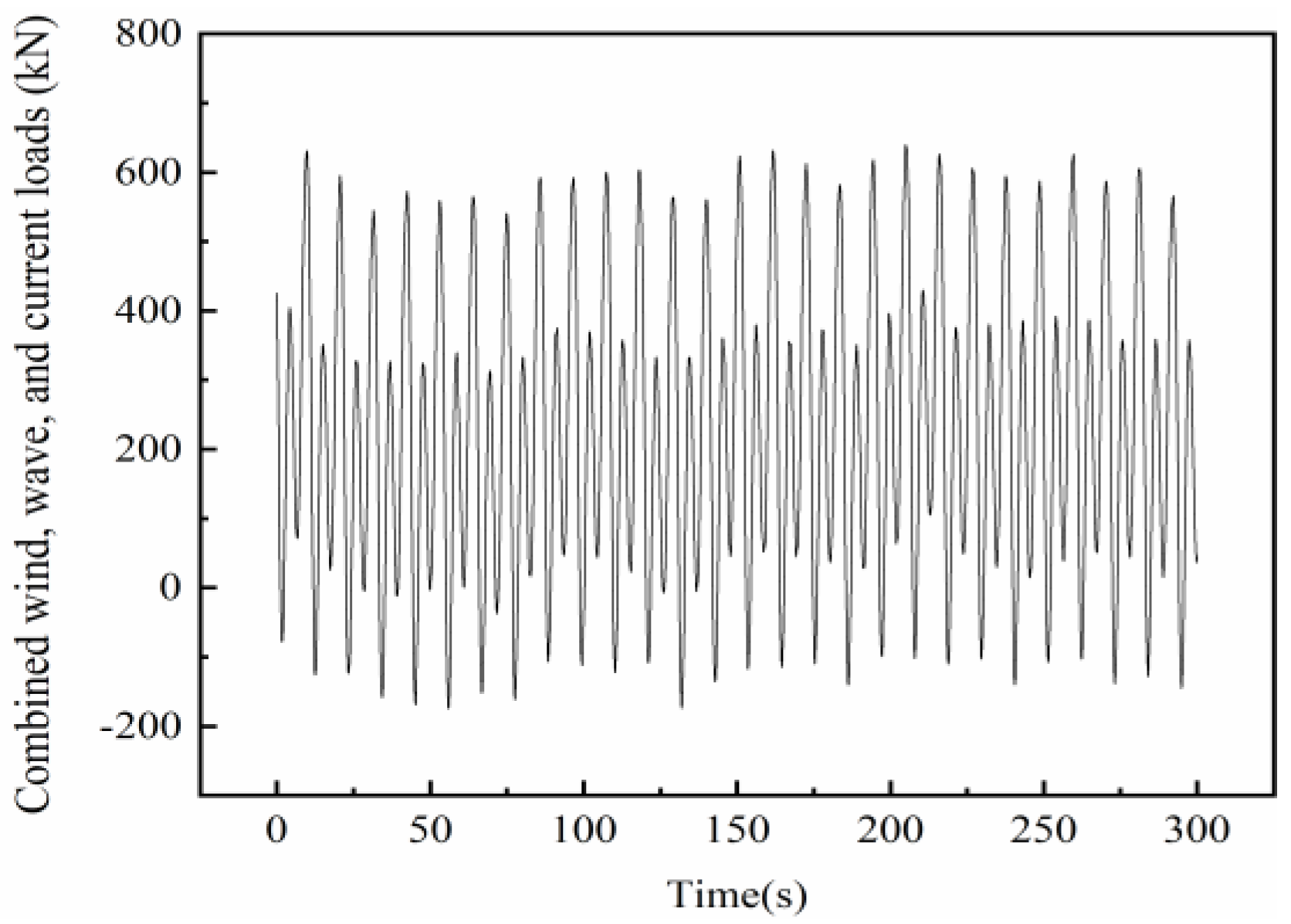
2.4.2. Combination and Simplification of Wind, Wave and Current

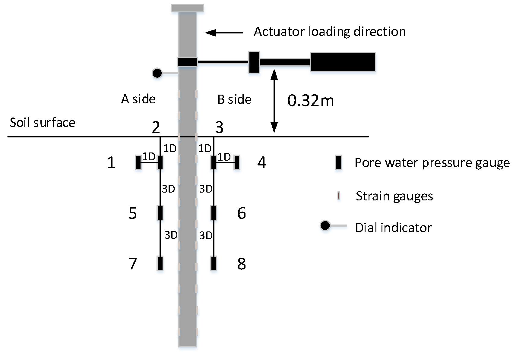
Based on the above load calculation theory, the time history data of wind load, wave and ocean current load are obtained, and then the horizontal loads of wind, wave and current on the wind turbine are combined and simplified according to the principle of equivalent bending moment.

Figure 5 is a schematic diagram of the load simplification process. According to Bhattacharya’s simplified method (2013) [4], the load on the overall wind turbine structure is divided into three parts. P₁ is the wind load on the blade, P₂ is the wind load on the tower, and P₃ is the wave and current load on the pile section below the water surface and above the mud surface. y₁, y₂, and y₃ are the acting heights of the respective resultant forces of the three types of loads. Since these three types of horizontal loads will generate a large overturning moment of the fan structure, if the bending moment is used as the equivalent condition, the three types of loads can be combined and equivalent, and the results are shown in the figure. According to the results of the simulation trial calculation, the three types of loads in the prototype site can reach the maximum value within the simulation time of 300 s, so the time history result of the simulation prototype site with a duration of 300 s is determined. The final combined and simplified wind, wave and current load results are shown in Figure 6. It represents the time history of the resultant force of the horizontal load of wind, wave and current on the prototype wind turbine.

2.5. Test Device

In previous similar experimental studies, researchers usually simplified the marine environmental load. The main focus is on the characteristics of the low-frequency cycle of wind, wave and current loads, and the completely one-way or two-way load form determined by experience is adopted, and only the regular action of equal-amplitude loads is considered. Therefore, the amplitude and frequency of the load cannot be changed arbitrarily in a certain test, but this is inconsistent with the actual sea state. In order to better solve this problem, a complex dynamic load loading system was independently developed in this experiment in the early stage of design. This loading system can apply the load time history results obtained by theoretical calculation to the model structure in a custom way, which can realize asymmetric and irregular ocean load loading.

As shown in Figure 7, the whole loading system is divided into four parts: model box, reaction frame, actuating device and data acquisition device. Because the iterative algorithm is embedded in the servo control system of the actuator, it can realize dynamic loading in a large frequency domain and meet the requirements of precisely controlling the load amplitude and frequency in this model test. The loading system can realize control methods such as force control and displacement control, so that the dynamic load time history obtained by theoretical calculation can be accurately applied to the model structure.

For dynamic loading model tests, boundary effects cannot be ignored. In the dynamic test, Nagomi et al. (2010) [21] proposed that when the distance between the model structure and the rigid boundary of the model box is greater than three times the pile diameter, the boundary effect caused by dynamic loading can be ignored. For the test conditions of this study, the distance between the bottom of the model pile and the bottom of the rigid box is 0.7 m, which is greater than ten times the pile diameter. The vertical distances between the model pile wall and the rigid box side wall are 0.47 m and 0.72 m, respectively, which are also greater than 7 times the pile diameter. Therefore, the dynamic loading boundary effect of the model test in this study can be ignored. The specific relative position relationship is shown in Figure 7.

The bending moment of the pile body during the test was monitored by 24 strain gauges arranged on both sides of the pile body, and the spacing between each two groups of strain gauges was 0.06 m. Among them, 1 pair is at the soil surface, 2 pairs are above the soil surface, and 9 pairs are below the soil surface. By arranging the strain gauges symmetrically on both sides of the pile body, the bending moment of the pile body of the pile section can be obtained by using the bending moment calculation method.

For the measurement of pore water pressure at different positions around the pile during the test, 8 pore water pressure gauges were used, and the arrangement of the pore pressure gauges adopted the arrangement suggested by Norris (2003) [22]. In the shallow soil, four pore water pressure gauges are arranged before and after the axis of the pile body, which are divided into two categories: far field and near field. Two pore water pressure gauges are arranged in the middle soil body and the deep soil body at the position of one pile diameter before and after the axis of the pile body, which are only arranged in the near field.

The above two types of test data are collected by the JM3841 dynamic strain acquisition instrument, and the sampling frequency of this model is 50 Hz; for the measurement of pile displacement and load, the dial indicator and the data acquisition system that comes with the actuator are used to collect. The distribution positions of the sensors in the whole test system are shown in Figure 8.

2.6. Design of Test Conditions

The design code for offshore wind turbines points out that there are four design states in the life of a single pile foundation, and these four design states correspond to the effects of the marine environment on the pile foundation under different working conditions. The ultimate load state (ULS) represents the effect of extreme wind and waves on the structure of the wind turbine, and the limit state during operation (SLS) corresponds to the impact of long-term loads on the operation of the wind turbine. According to the research purpose of this study, the two design states are used as the basis for determining the working conditions and the experiments are designed.

In a series of tests, Leblanc (2010) [23] and others proposed that there is a certain relationship between the static ultimate bearing capacity F_R of a single pile foundation and the maximum cyclic load F_max. According to the conclusion of its test, the static ultimate bearing capacity F_R and the maximum cyclic load F_max have the following relationship, and the cyclic load ratio ξ is defined as:

$$\xi =\frac{F_{max}}{F_R}$$

(10)

When ξ = 0~30%, corresponding to the design stage of the limit state (SLS) of the single pile foundation during operation, it represents the load condition of the prototype wind turbine structure under the long-term action of normal wind and waves; When ξ = 30~50%, corresponding to the design stage of the single pile foundation in the ultimate bearing state (ULS), it represents the load condition of the prototype wind turbine structure under the short-term action of extreme wind and waves.

According to the above test conclusions, before determining the dynamic load amplitude, it is necessary to carry out a static loading test to determine the static limit load FR of the pile–soil system used in the test, which provides a basis for the determination of the amplitude Fmax in the subsequent dynamic test. Due to the high loading frequency of the dynamic test, in order to ensure that the pore water pressure can be clearly observed during the entire test process, the undrained rate suggested by the University of Western Australia (1994) [24] was used for loading, and the final loading rate was 1 mm/s. According to the test conclusion of Leblanc, in the test group under the short-term action of extreme wind and waves, the cyclic load ratio ξ is 0.3, 0.4, and 0.5, respectively; in the long-term action test group with normal wind and waves, the cyclic load ratio ξ is 0.1, 0.2, and 0.3, respectively. The specific test conditions are shown in

Table 2. Test conditions.

Test Conditions	Group Number	ξ	Cycle Times	Control Method Category
Static loading	S1	1 mm/s (Loading rate)	/	Displacement control
Extreme wind and wave short-term conditions	D1	0.3	27	Force control
	D2	0.4	27	Force control
	D3	0.5	27	Force control
Normal wind and wave long-term conditions	L1	0.1	5000	Force control
	L2	0.2	5000	Force control
	L3	0.3	5000	Force control

.

3. Analysis of Discussion

3.1. Analysis of Static Loading Test Results

In order to determine the horizontal ultimate bearing capacity of the offshore wind turbine monopile foundation model under the action of horizontal loads, a static loading test is firstly carried out. Because the failure and damage of offshore wind turbine foundations are usually characterized by excessive deformation, the excessive deformation of the foundation at the mud surface will cause the wind turbine to take protective measures and stop running. Therefore, the pile foundation reaction force corresponding to a certain displacement at the test loading point is taken as the ultimate bearing capacity of the existing pile–soil system. This study comprehensively considers the actual site conditions and model test conditions and is based on the field test conclusions of Borms (1964) [25]. When 0.2D displacement occurs at the loading point, the pile foundation reaction force collected by the actuator pressure sensor is the horizontal ultimate bearing capacity of the pile–soil system. According to the test situation in this study, the static ultimate bearing capacity of the pile–soil system in this model test is 263 N.

The strain of the pile body during the test can be obtained by the strain gauges arranged on both sides of the pile body, and then the bending moment of the pile body during the loading process can be obtained by the bending moment calculation method proposed by Liang (2006) [26]. In the process of model test, because the soil pressure of pile–soil interaction below the mud surface is not easy to measure, according to the knowledge of material mechanics, there is a certain mathematical relationship between the bending moment of the pile and the radius of curvature of the pile. Therefore, the displacement of the pile body, the bending moment of the pile body and the resistance of the surrounding soil can be calculated by mutual derivation. Zhu (2015) [27] et al. verified the feasibility of deriving displacement and soil resistance from the measured pile body bending moment. In this study, the same method is used to obtain the expression of the bending moment from the discrete data of the pile body bending moment six times, and then the second difference of the expression can be used to obtain the result of the soil resistance around the pile in this test.

Figure 9 shows the results of the distribution of soil pressure around the pile along the depth obtained by the second difference of the bending moment of the pile body. According to the results shown in the figure, the displacement area of the entire pile body under the action of horizontal load can be divided into a passive area where the pile and soil squeeze each other (the upper part of the A side and the lower part of the B side around the pile) and the active area where the pile and soil tend to be separated (the pile around A side lower and B side upper). It can be seen from the figure that the distribution forms of soil resistance under different load levels are basically the same. From the mud surface to the bottom of the pile, the overall curve of soil resistance first increases and then decreases, gradually decreases to zero, and then increases to trend of maximum value. The displacement of the pile body and the resistance of the soil are both zero at the inflection point of the curve, which can be regarded as the rotation center under the static load, and the position of the rotation center is approximately 6 times the pile diameter under the soil surface. With the increase in depth, in the area above the rotation center, the soil resistance around the pile gradually reaches the maximum value, then gradually decreases from the peak value, and decreases to zero near the rotation center. From the perspective of different loading levels, the soil resistance of the soil near the passive zone will increase with the increase in the load, which is consistent with the experimental results of Zhu.

Figure 10 shows the soil resistance of the pile body and the displacement of the pile body through quadratic differentiation and difference after fitting the measured bending moment data. Finally, the graph of the change of soil resistance around the pile with the horizontal displacement of the pile body at different depths (1D~4D) of the soil body is obtained, and 1D~4D in the figure represents the depth of the soil layer from the soil surface. It can be seen from the figure that with the increase in the horizontal displacement of the pile body, the soil resistance at different depths under various loads gradually increases, but the development trend of soil resistance does not slow down whether it is the surface layer or the deep soil. When the soils at different depths have the same displacement, the soil resistance of the deep soils increases more. When the soils at different depths reach the same soil resistance, the displacements of the shallow soils are larger than those of the deep soils.

It can be seen from the above analysis that the whole pile body rotates around the rotation center at 6 times the pile diameter below the mud surface (approximately 0.35 m below the mud surface). According to the arrangement position of the test sensor. Pore water pressure gauges No. 1, 2, 3 and 4 are located in the shallow soil around the pile, pore water pressure gauges No. 5 and 6 are located in the middle soil body, and pore water pressure gauges No. 7 and 8 are located in the deep soil body. For No. 1, 2, 5 and No. 8 pore water pressure gauges, it is located in the passive area where the pile body and the soil body squeeze each other. For No. 3, 4, 6 and 7 pore water pressure gauges, it is located in the active area where the pile body and the soil tend to separate from each other.

Figure 11 shows the test results of the pore water pressure at different positions around the pile in the shallow soil in the static load model test. During the test, at the position of the No. 1 and No. 2 piezometers on the front side of the pile body, when the pile body is subjected to an external load, the soil on the front side of the pile body is squeezed, so the pore water pressure at this position rises. When the loading is stopped, the pore water pressure of the soil at the surface dissipates rapidly. For the No. 3 and No. 4 piezometers on the back of the pile body, due to the action of horizontal load, the pile and soil are separated, and the gap between the pile body and the soil is quickly filled with water. When the pile body continues to move forward, the soil behind the pile produces negative pore pressure. With the increase in the displacement of the pile body, the negative pore pressure of the soil at the positions of the No. 3 and No. 4 piezometers behind the pile also increases gradually. The pore pressure of the No. 3 piezometer, which is closer to the pile body, has a greater increase. Because the closer to the pile, the greater the soil displacement and the greater the negative hole pressure. As the loading stops, the pore water redistribution in the soil causes the pore water pressure to gradually fall back to the hydrostatic pressure value at the water level.

Figure 12 shows the results of the pore water pressure in the soil measured by arranging pore pressure gauges at the same distance and different depths on the A side of the pile body during the model test. The positions of the 2, 5 and 7 hole pressure gauges in the figure are shown in Figure 4. As shown in the results in the figure, the pore pressures monitored by No. 2 and No. 5 porosimeters gradually increased as the loading progressed. However, due to the tendency of the pile body to deviate from the soil, suction is generated at the position of the No. 7 pore pressure gauge, and the negative pore water pressure at this position also gradually increases. Judging from the absolute value of pore water pressure, the pore water pressure of No. 7 porosimeter is not as large as that of No. 2 and No. 5 porosimeters. It may be due to the fact that the deep soil body has a large constraint on the pile, and the displacement generated under the load is small.

Similarly, Figure 13 shows the results of the pore water pressure in the soil measured by arranging piezometers at the same distance from the pile body and at different depths in the soil behind the pile. It can be seen from the figure that the soil at the 3 and 6 hole pressure gauge positions behind the pile body generates suction due to the separation of the pile and soil. Moreover, as the loading progresses, the pore water pressures at both positions increase, but the pore pressure of the No. 3 pore pressure gauge in the shallow soil body and the No. 6 pore pressure gauge in the middle soil body are not consistent. It may be due to the fact that the porosimeter in the topsoil is closer to the water surface, and the voids at the mud surface are larger, so the measured pore water pressure is not as large as that of the middle soil. However, the pore pressure changes measured by the No. 8 pore pressure gauge at the deeper soil body are consistent with the aforementioned situation. The soil in front of the pile is squeezed at this position, and the pore water pressure has increased.

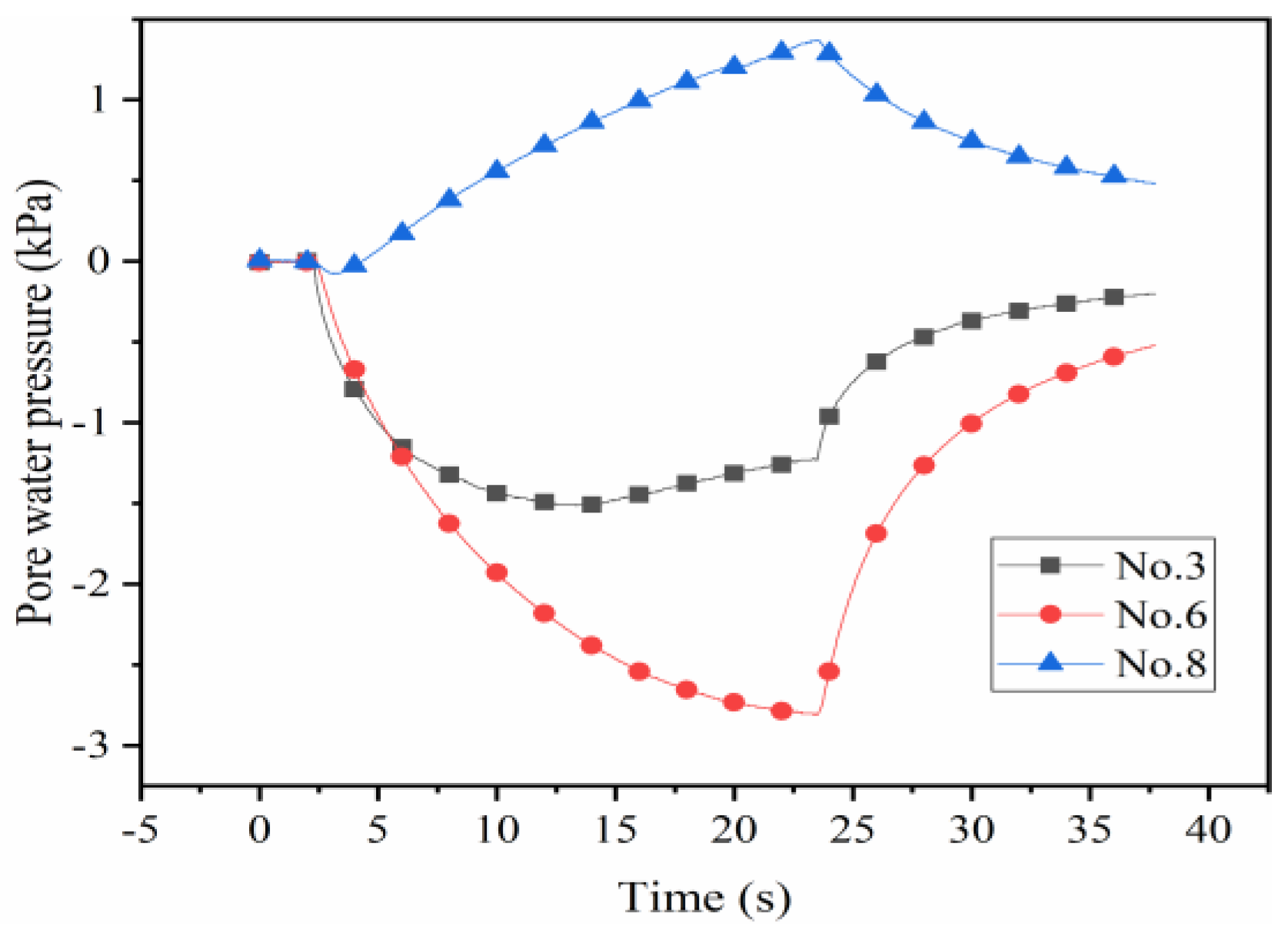
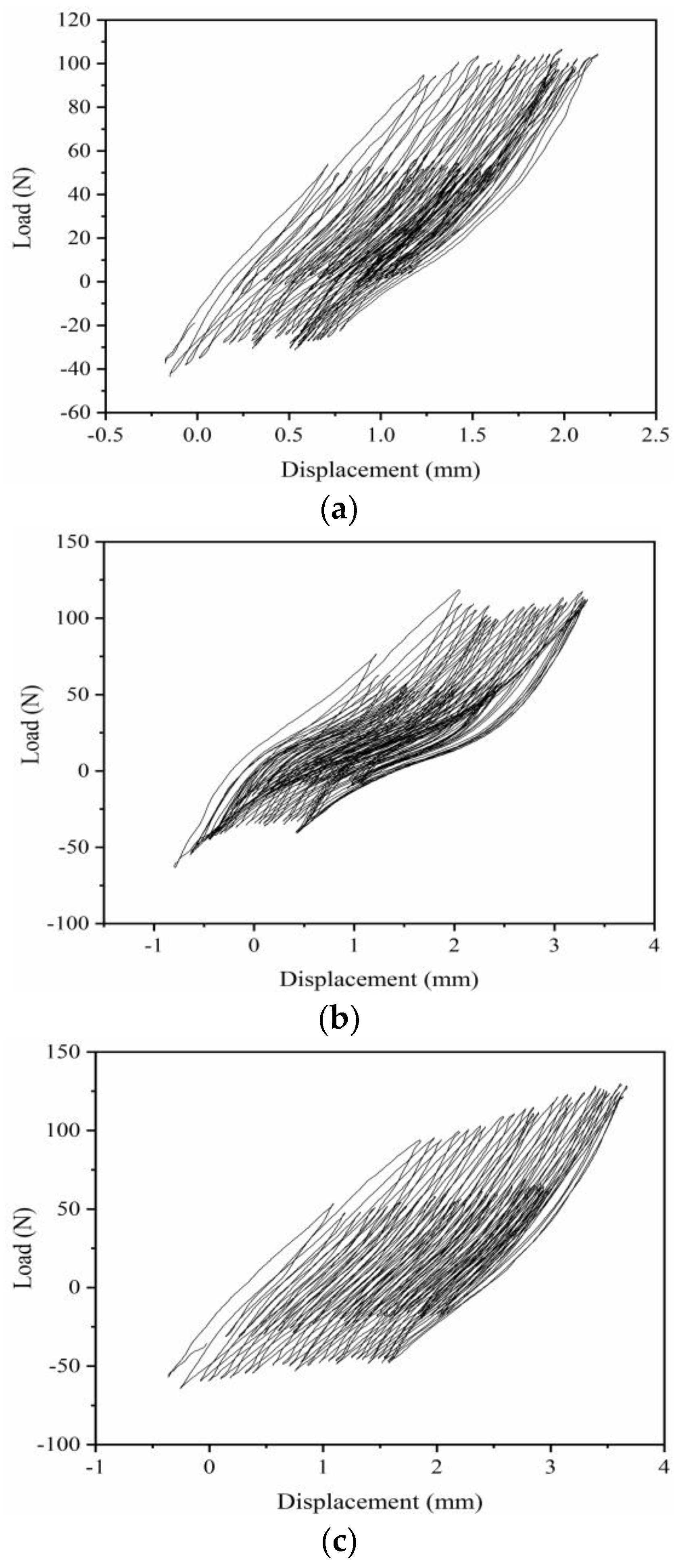
3.2. Analysis of Short-Term Effect Test Results of Extreme Wind, Wave and Current

This section is based on the experimental conditions designed in Table 2 and the calculation parameters of wind, wave and current under the prototype sea conditions. Three groups of model tests were carried out on the mechanical properties of the offshore wind turbine monopile foundation in the ultimate load state stage (SLS). The dynamic response of the offshore wind turbine monopile foundation under extreme wind and wave currents is obtained.

Figure 14a–c show the load–displacement test results of groups D1, D2, and D3 under extreme wind and wave currents. This group of tests simulates the short-term effects of extreme wind, wave and current loads in the marine environment. It can be seen from the figure that the development process of the pile body displacement is basically the same as the load form, indicating that the load action form has a great influence on the displacement development. At the same time, it can be seen that the density of the load–displacement curve does not change significantly at the initial stage of loading and the later stage of loading, indicating that the displacement of the pile body has maintained a rapid development trend under the short-term action of extreme wind, wave and current loads. In practical engineering, when the wind turbine structure is subjected to short-term extreme wind and waves, the displacement of the pile body will develop rapidly. Therefore, a shutdown strategy should be adopted in time to reduce the load on the blades, thereby reducing the displacement development rate of the pile foundation structure.

Figure 15 shows the variation of pore water pressure at the position of No. 1 piezometer in the soil around the pile body in the model test. It can be seen from the figure that in the whole test process, the change trend of pore pressure is basically consistent with the change form of load. At the same time, it can be seen that the peak pore pressure at the position of the No. 1 pore pressure gauge has a certain increase with the action of the simulated wind, wave and current load. However, since the pore pressure gauge is located in the surface soil at a depth of 1 times the pile diameter from the soil surface, the increase in pore pressure caused by the drainage effect is not obvious.

Figure 16 shows the change of pore water pressure in the soil around the pile measured by the No. 2 piezometer which is close to the pile body. Compared with the No. 1 piezometer, because the vertical distance from the pile body is shorter, the soil at this position has a greater response to the load, so the resulting displacement is more significant. The overall pore water pressure change amplitude is significantly higher than the monitoring value of No. 1 porosimeter. The overall fluctuation form of pore pressure is still basically consistent with the load form. Due to the short distance from the pile body, the reciprocating motion of the pile foundation will cause a drainage channel between the pile body and the soil body, resulting in contact seepage. Therefore, the accumulation of pore pressure is still not obvious, but the peak pore pressure has a certain increase.

Figure 17 shows the variation of pore water pressure of the soil around the pile at the position of the No. 8 piezometer located in the deep soil in the model test. It can be seen from the figure that the accumulation of soil pore water pressure at No. 8 piezometer. When the load begins to act, the soil around the pile on both sides of the pile body is continuously compacted, the change trend of the excess pore water pressure is consistent with the load fluctuation and continues to accumulate, and the excess pore water pressure gradually increases. However, after a certain number of loads, the accumulation of excess static pore water pressure gradually becomes flat due to the gradual compaction of the soil around the pile. With the stop of loading, the excess static pore water pressure of the soil around the pile appears to drop immediately. This test result is consistent with the law that the pore water pressure of the seabed foundation soil will increase cumulatively when the single pile in the saturated sand foundation is subjected to extreme wind and wave current loads in the actual project.

The results of the pore water pressure measured by the porosimeters at 8 different positions in Figure 8, and the results of the distribution of the maximum pore water pressure at each position along the depth are drawn in Figure 18. Since the soil surface is drained, the pore water pressure on the soil surface is zero. It can be seen from Figure 18 that, in general, the pore water pressure in the soil around the pile shows a trend of first increasing and then decreasing along the change of soil depth. At the same time, the smaller the vertical distance from the pile, the greater the variation of pore pressure, as shown in the results of pore pressure gauges 2 and 3. At the same vertical distance from the pile, the pore pressure amplitude of the shallow soil is greater than that of the deep soil. As shown, the results of porosimeter 2 are greater than those of porosimeters 5 and 7 and the results of porosimeter 3 are greater than those of porosimeters 6 and 8.

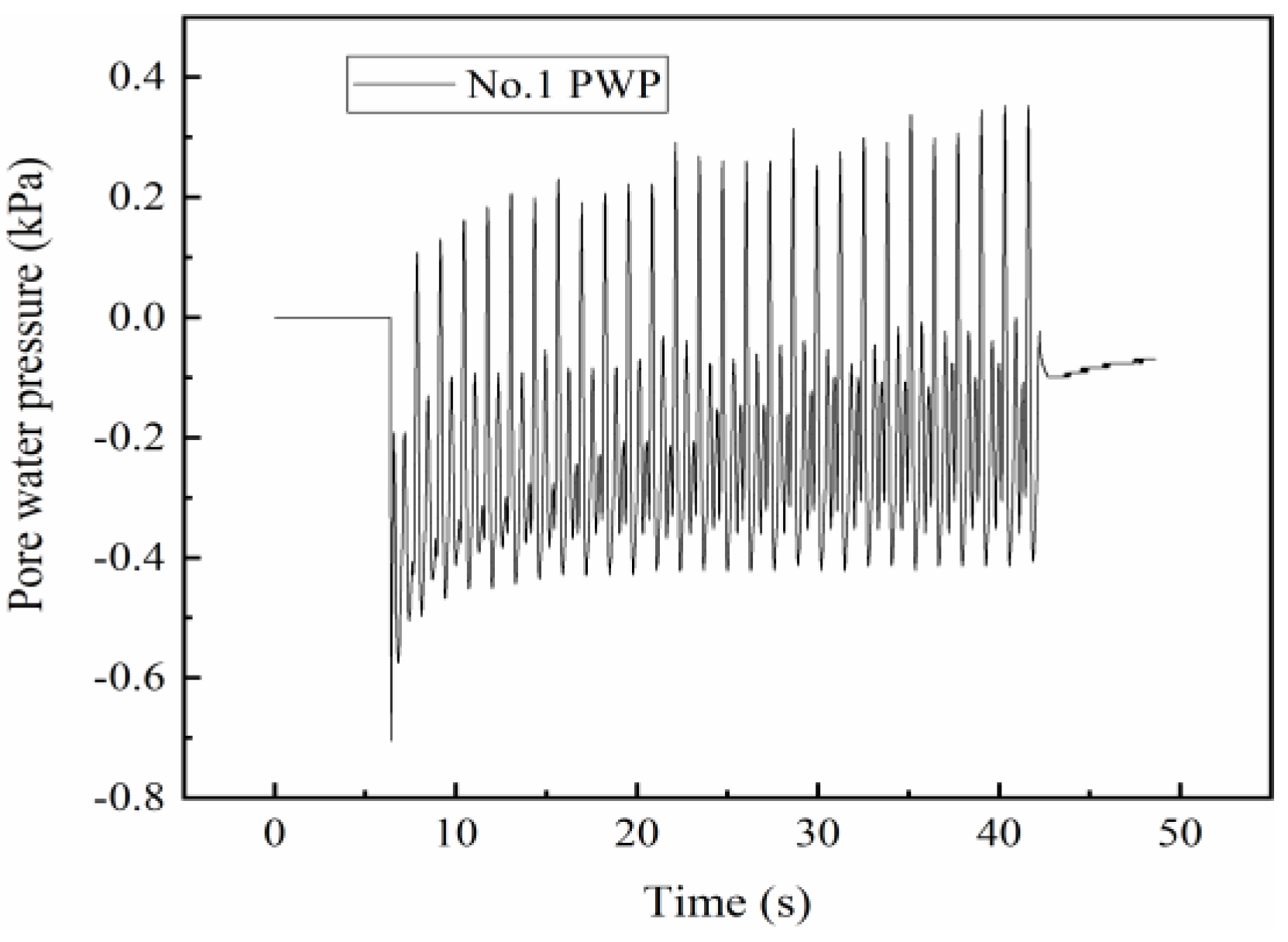
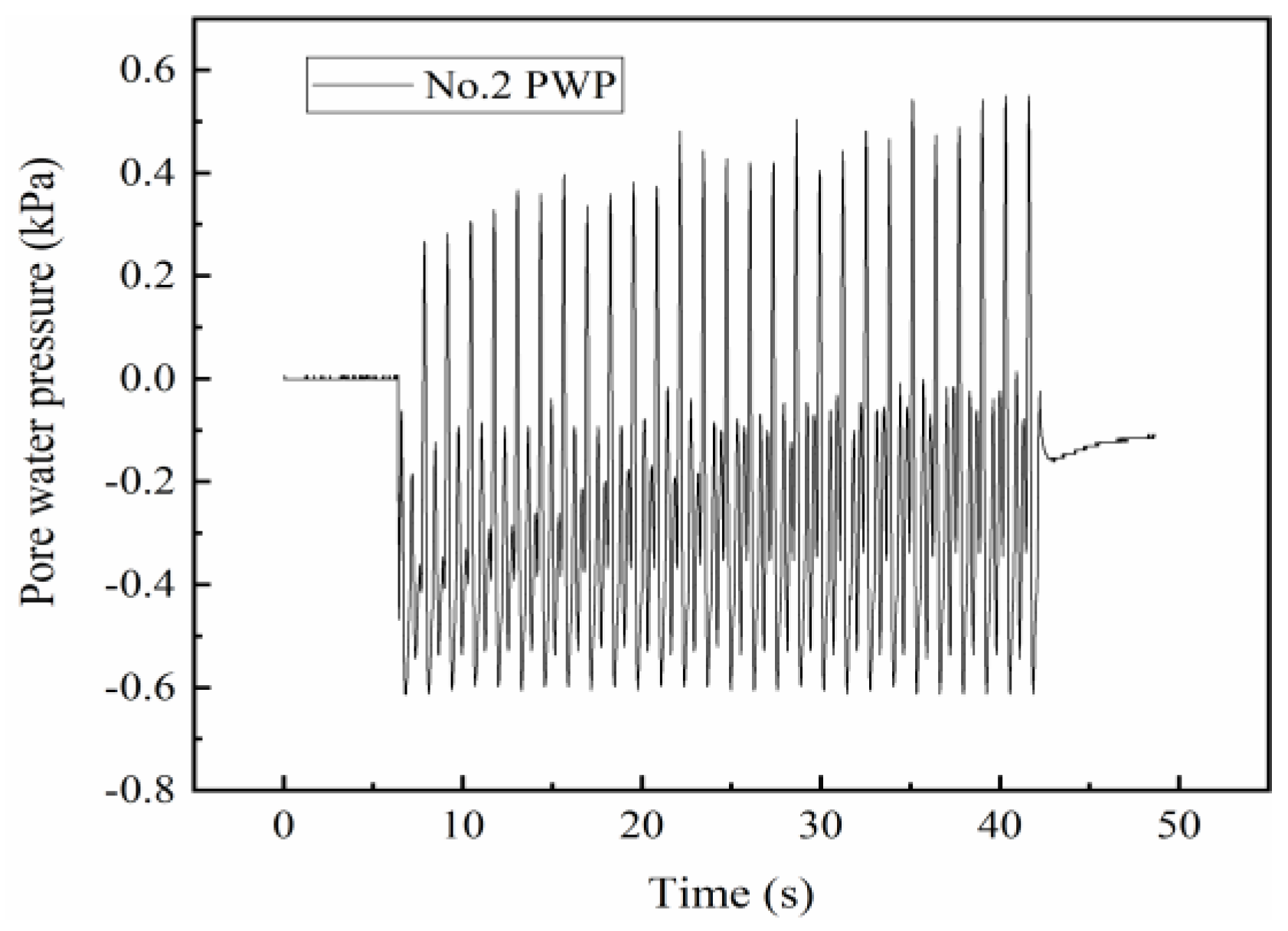
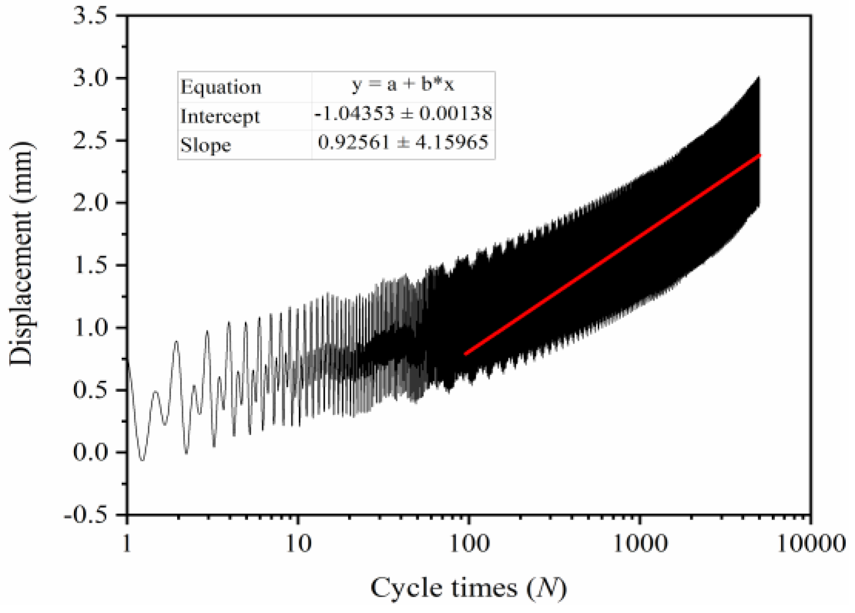
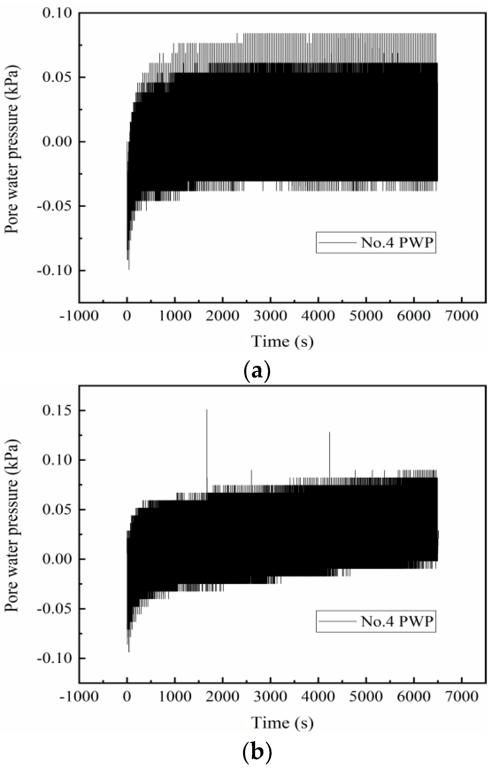
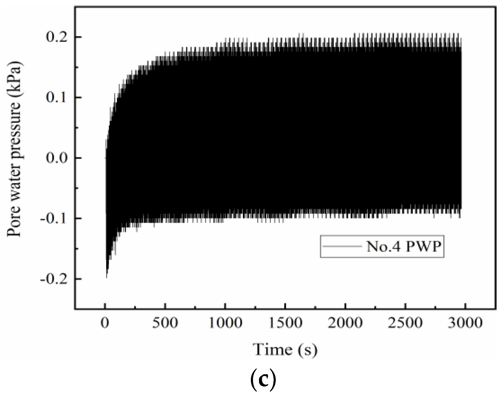
3.3. Analysis of Long–Term Effects of Normal Wind, Wave and Current on Test Results

This set of test conditions is to simulate the working state of the wind turbine foundation under the long-term action of normal wind and waves, so as to investigate the dynamic response of the wind turbine monopile foundation under the long-term cyclic action of wind, wave and current loads.

Based on the load calculation results of the prototype fan, the amplitude of the final resultant force is kept close to the design amplitude of the cyclic load in this group of test conditions by adjusting the load parameters. The above cyclic loads were then applied to the model structure for approximately 5000 cycles.

Taking the test results of L2 test group (cyclic load ratio ξ = 20%) as an example, the displacement development results of pile body are explained. It can be seen from Figure 19 that the accumulated displacement of the pile body develops rapidly in the early stage of loading (the first 500 s) due to the gradual displacement of the single-pile foundation to the A side under the action of the cyclic load. However, in the later stage of loading, the increasing rate of the cumulative displacement of the pile body gradually decreases, and the overall displacement curve tends to be flat. From the details of the displacement results, the development trend of the displacement is still consistent with the form of the load.

Figure 20 shows the hysteresis curve of horizontal load displacement when simulating normal wind, wave and current load for a long time, taking the L3 test group with the cyclic load ratio ξ as 30% as an example. It can be seen from the load–displacement curves of this group that with the progress of cyclic loading, the area of the hysteresis loop of the load–displacement curve gradually decreases under the same number of loads. It shows that the displacement development rate of the pile body will gradually decrease with the increase in the number of cycles under the long-term load.

Figure 21 shows the relationship between the cumulative displacement of group L2 and the logarithm of the number of cycles. Due to the limited number of load actions in the model test, it is impossible to truly restore the high-cycle cyclic load action of the actual fan during operation. According to some current research conclusions, the cumulative displacement empirical formula can be used to predict the pile displacement development under the long-term action of wind and waves. Due to the irregularity of the load in this test (there are both large and small wave peaks), it is difficult to extract the peak-finding data, so only the relationship between the overall displacement at the loading point and the number of cyclic actions is analyzed.

Figure 22a–c, respectively, show the changes of excess pore water pressure monitored by No. 4 porosimeter in the soil under the three working conditions during the long-term circulation of wind, wave and current. It can be seen from the figure that in the initial period of loading, the pore pressures measured in the three groups of tests are all negative values. This is because the pile body vibrates under the load at the initial stage of the load, and a certain gap is generated between the pile and the soil, thereby generating a negative pore pressure. After that, with the action of long-term load, the overall pore water pressure of the soil in the middle of the pile showed an upward trend, but after a certain number of cycles, the increase in the pore pressure tends to a stable value, and the pore water pressure still cyclically fluctuates with the action of the load. The variation trend of pore water pressure of No. 4 porosimeter in the three groups of tests is similar, but the results of pore pressure are different due to different load amplitudes.

4. Conclusions

In this study, the dynamic loads are calculated based on the wind, wave and current load theory, the model test is carried out through the self-developed complex dynamic load loading system, the dynamic response of the monopile foundation under the complex marine load is investigated, and the following conclusions are obtained. The results show that the accurate simulation of wind, wave and current load calculated theoretically in this study can be realized through the loading device, and the characteristics of marine environmental load are considered more comprehensively. Therefore, the pile–soil dynamic response obtained by the test method in this study is closer to the impact of actual marine environmental load on the offshore wind turbine structure.

References

1. Xu, L.Y.; Song, C.X.; Chen, W.Y. Liquefaction-induced settlement of the pile group under vertical and horizontal ground motions. Soil Dyn. Earthq. Eng. 2021, 144, 106709. [Google Scholar] [CrossRef]
2. Chen, W.; Huang, L.; Xu, L.; Zhao, K.; Wang, Z.; Jeng, D. Numerical study on the frequency response of offshore monopile foundation to seismic excitation. Comput. Geotech. 2021, 138, 104342. [Google Scholar] [CrossRef]
3. Frick, D.; Achmus, M. An experimental study on the parameters affecting the cyclic lateral response of monopiles for offshore wind turbines in sand. Soils Found. 2020, 60, 1570–1587. [Google Scholar] [CrossRef]
4. Lombardi, D.; Bhattacharya, S.; Wood, D.M. Dynamic soil-structure interaction of monopile supported wind turbines in cohesive soil. Soil Dyn. Earthq. Eng. 2013, 49, 165–180. [Google Scholar] [CrossRef]
5. Pan, D.; Lucarelli, A.; Cheng, Z. Field test of monopile for offshore wind turbine foundations. In Proceedings of the Geotechnical and Structural Engineering Congress 2016, Phoenix, AZ, USA, 14–17 February 2016. [Google Scholar]
6. Zhu, B.; Yang, Y.Y.; Yu, Z.G.; Guo, J.F.; Chen, Y.M. Field tests on lateral monotonic and cyclic loadings of offshore elevated piles. Chin. J. Geotech. Eng. 2012, 34, 1028–1037. [Google Scholar]
7. Romijnders, L.N.G. The Development of a New Segmented Deepwater Wave Generator. In Proceedings of the Fourth International Symposium on Ocean Wave Measurement and Analysis, San Francisco, CA, USA, 2–6 September 2001. [Google Scholar]
8. Utsunomiya, T.; Sato, T.; Matsukuma, H.; Yago, K. Experimental Validation for Motion of a SPAR-Type Floating Offshore Wind Turbine Using 1/22.5 Scale Model. In Proceedings of the ASME International Conference on Ocean, Honolulu, HI, USA, 31 May–5 June 2009. [Google Scholar]
9. Eitaro, N.; Tomoaki, U.; Iku, S. Irregurar wave experiment on motion of floating foundations of cylindrical shape for offshore wind turbine. Proc. Civ. Eng. Ocean 2008, 24, 135–140. [Google Scholar]
10. Hansen, N.M. Interaction between Seabed Soil and Offshore Wind Turbine Foundations. Ph.D. Thesis, Danmarks Tekniske Universitet, Copenhagen, Denmark, 2012. [Google Scholar]
11. Kuo, Y.S.; Achmus, M.; Abdel-Rahman, K. Minimum embedded length of cyclic horizontally loaded monopiles. J. Geotech. Geoenvironmental Eng. 2012, 138, 357–363. [Google Scholar] [CrossRef]
12. Buckingham, E. The principle of similitude. Nature 1915, 96, 396–397. [Google Scholar] [CrossRef] [Green Version]
13. Cuéllar, V.P. Pile Foundations for Offshore Wind Turbines: Numerical and Experimental Investigations on the Behavior under Short-Term and Long-Term Cyclic Loading. Ph.D. Thesis, Technischen Universität Berlin, Berlin, Germany, 2012. [Google Scholar]
14. Poulos, H.G.; Hull, T.S. The Role of Analytical Geomechanics in Foundation Engineering. Foundation Engineering: Current Principles and Practices; ASCE: Reston, VA, USA, 1989. [Google Scholar]
15. Ovesen, N.K. The use of physical models in design: The scaling law relationship. In Proceedings of the 7th European Conference on Soil Mechanics and Foundation Engineering, Brighton, UK, September 1979; Volume 4, pp. 318–323. [Google Scholar]
16. Kareem, A.; Kijewski, T. Time-frequency analysis of wind effects on structures. J. Wind. Eng. Ind. Aerodyn. 2002, 90, 1435–1452. [Google Scholar] [CrossRef]
17. Simiu, E.; Scanlan, R.H. Wind effects on structures: An introduction to wind engineering. Arch. Proc. Inst. Mech. Eng. 1970, 185, 301–317. [Google Scholar]
18. Davenport, A.G. The relationship of reliability to wind loading. J. Wind. Eng. Ind. Aerodyn. 1983, 13, 3–27. [Google Scholar] [CrossRef]
19. Zhang, X.L.; Liu, J.X.; Han, Y.; Du, X.L. A framework for evaluating the bearing capacity of offshore wind power foundation under complex loadings. Appl. Ocean. Res. 2018, 80, 66–78. [Google Scholar] [CrossRef]
20. Méhauté, B.L.; Divoky, D.; Lin, A. Shallow water waves: A comparison of theories and experiments. Coast. Eng. Proc. 1968, 1, 7. [Google Scholar] [CrossRef]
21. Nogami, T.; Novak, M. Resistance of soil to a horizontally vibrating pile. Earthq. Eng. Struct. Dyn. 2010, 5, 249–261. [Google Scholar] [CrossRef]
22. Ashour, M.; Norris, G. Lateral loaded pile response in liquefiable soil. J. Geotech. Geoenviron. Eng. 2003, 129, 404–414. [Google Scholar] [CrossRef]
23. Leblanc, C.; Houlsby, G.T.; Byrne, B.W. Response of stiff piles in sand to long-term cyclic lateral loading. Géotechnique 2010, 60, 79–90. [Google Scholar] [CrossRef]
24. Stewart, D.P.; Randolph, M. T-Bar Penetration Testing in Soft Clay. J. Geotech. Eng. 1994, 120, 2230–2235. [Google Scholar] [CrossRef]
25. Broms, B. Lateral resistance of piles in cohesionless soils. ASCE Soil Mech. Found. Div. J. 1964, 90, 123–156. [Google Scholar] [CrossRef]
26. Yang, K.; Liang, R. Methods for deriving p-y curves from deviceed lateral load tests. Geotech. Test. J. 2006, 30, 1–8. [Google Scholar]
27. Zhu, B.; Sun, Y.X.; Chen, R.P.; Guo, W.D.; Yang, Y.Y. Experimental and Analytical Models of Laterally Loaded Rigid Monopiles with Hardening p-y Curves. J. Waterw. Port Coast. Ocean. Eng. 2015, 141, 04015007. [Google Scholar] [CrossRef]
Figure 1. The grain-size distributions curve.
Applsci 12 05197 g001
Figure 2. Steel pipe pile and model structure.
Applsci 12 05197 g002
Figure 3. Time history curve of wind load at fan hub.
Applsci 12 05197 g003
Figure 4. Time history curve of wave and current.
Applsci 12 05197 g004
Figure 5. The simplified diagram of load.
Applsci 12 05197 g005
Figure 6. The result of combined wave and current load.
Applsci 12 05197 g006
Figure 7. Sketch map of test device.
Applsci 12 05197 g007
Figure 8. Sensor layout position and loading direction.
Applsci 12 05197 g008
Figure 9. The distribution of soil resistance around pile.
Applsci 12 05197 g009
Figure 10. The soil resistance and horizontal along depth displacement curves at different depths.
Applsci 12 05197 g010
Figure 11. The pore water pressure in shallow soil.
Applsci 12 05197 g011
Figure 12. The pore water pressure at different depths.
Applsci 12 05197 g012
Figure 13. The pore water pressure at different depthson side A on side B.
Applsci 12 05197 g013
Figure 14. The load–displacement curves. (a) The load–displacement curve of Group D1; (b) the load–displacement curve of Group D2; (c) the load–displacement curve of Group D3.
Applsci 12 05197 g014
Figure 15. The results of No. 1 pore pressure gauge.
Applsci 12 05197 g015
Figure 16. The results of No. 2 pore pressure gauge.
Applsci 12 05197 g016
Figure 17. The results of No. 8 pore pressure gauge.
Applsci 12 05197 g017
Figure 18. Distribution of the maximum pore water pressure along depth.
Applsci 12 05197 g018
Figure 19. Cumulative displacement development.
Applsci 12 05197 g019
Figure 20. Load–displacement hysteresis curve of L2 groups under long-term load.
Applsci 12 05197 g020
Figure 21. Relationship between cumulative displacement and cycle times of group L2.
Applsci 12 05197 g021
Figure 22. The pore water pressure in middle soil. (a) The results of No. 4 pore pressure gauge of Group L1; (b) the results of No. 4 pore pressure gauge of Group L2; (c) the results of No. 4 pore pressure gauge of Group L3.
Applsci 12 05197 g022aApplsci 12 05197 g022b