Using a Machine Learning Method to Predict the Penetration Depth of a Gravity Corer

Abstract

The study of penetration depth of gravity piston samplers has an essential impact on sampling efficiency and instrument safety. This study focuses on predicting penetration depth based on the characteristic parameters of the sampled seafloor sediments and the sampler parameters. Although numerous studies of gravity corer penetration depth have been carried out, most have been based on the energy conservation equation, which considers a varying number of influencing factors. Furthermore, most research has focused on the same research idea of finding analytical solutions. The present study proposes a new approach to predicting gravity corer penetration depth based on a machine learning method that uses real sampling data from the sea and experimental data from a gravity sampling physical model for training and testing. Experimental results indicate that the machine learning model can accurately predict gravity corer penetration depth. Moreover, predictions were made for the same penetration conditions using the machine learning model and three other analytical solution models. Results show that the prediction accuracy of machine learning outperforms that of the analytical prediction model under various statistical rubrics. This study demonstrates the capacity of the proposed machine learning model and provides civil engineers with an effective tool to predict the penetration depth of gravity corers.

1. Introduction

A gravity piston sampler is an important geological tool that uses its gravity as the driving force to obtain in situ samples. Since the design proposal of the Kullenberg-type gravity sampler in 1947 [1], it has been widely used for the acquisition of deep-sea ultra-long in situ samples [2,3], nearshore sediment samples [4], and in situ lake sediment samples [5]. In recent years, due to the research and development of gas hydrate, the acquisition of high-fidelity in situ samples based on a gravity piston sampler [6,7,8] has become a hot research topic. Whether for the acquisition of deep-sea, nearshore, or lake sediments, how to improve the sampling efficiency and ensure continuous and undisturbed sediment samples have been the focus of much research. When sampling with a gravity piston sampler, the length of the installed sampling tube may be different from the actual penetration depth, which could lead to accidents, such as breakage of the sample tube when the size of the sample tube is greater than the penetration depth or failure to obtain the maximum length of a continuous in situ sample [9] when the size is less than the penetration depth. Therefore, the prediction of penetration depth according to the geological characteristics of the sampling area before the release of the gravity sampler can help improve the safety and efficiency of the sampler.

In previous studies of gravity sampler penetration depth, scholars mainly used force analysis and energy conservation to study analytical solutions. Li et al. [10] and Du et al. [9] obtained the analytical solution of the penetration depth equation based on the energy conservation equation through force analysis of the gravity sampler. They verified it with actual offshore sampling data. However, due to the complicated penetration process in the sampling area and problems of recording and operating errors in the real measured data at sea, the measured penetration data were not accurate, and the amount of data was small. To study the penetration process and factors of gravity samplers more accurately and controllably, Du [11] designed a gravity sampling physical test model in 2014 to address the problem of the small amount of data and lack of accurate data recording of the penetration process, conducted dozens of sets of tests, obtained a large amount of accurately recorded data, and proposed a new analytical solution model based on the tests. In recent years, scholars have also tried to discuss more influencing factors of gravity sampling penetration depth, such as friction coefficient and sediment characteristics [12,13]. However, the basic idea of past research was still to use the energy balance of penetration work and friction consumption work to solve the equation to determine the penetration depth, and there has been no substantial breakthrough in the modeling tools but only reduces the error value by parameters with less influencing factors. The complexity of the sampler penetration process, inaccuracies and other factors, and errors caused by human operation remain challenges to be eliminated. Therefore, there is an urgent need to propose a new means to model and study the penetration depth of gravity samplers.

Machine learning, the best-known class of artificial intelligence algorithms, is capable of efficiently approaching a wide range of data problems. Machine learning is divided into two main categories: supervised machine learning and unsupervised machine learning [14]. Supervised machine learning is used for training data with outcome labels, and unsupervised machine learning filters feature data, clustering without outcome labels. Supervised machine learning is further divided into two types of problems, classification and regression, depending on the result labels. Classification applies to data with a definite outcome, and regression applies to data with an uncertain type of outcome. Machine learning and deep learning techniques have been proven to be robust and promising tools in many geotechnical applications, such as ground motion prediction [15], soil liquefaction [16,17], landslides risk assessment [18,19,20,21], soil spatial prediction [22], soil hydraulic properties [23], geophysical exploration [24,25,26], etc. The above studies show that geological problems with a certain amount of data are well suited to be solved by machine learning methods. As for the gravity sampling penetration depth, it is more appropriate to choose the regression method in supervised machine learning because of its many influencing factors and the characteristic that the penetration depth results in data rather than categories. However, no one has yet conducted a gravity sampling penetration depth study using a machine learning approach. Machine learning methods can be applied to gravity sampling penetration depth studies, and the accuracy of the model predictions is the focus of this paper.

In this context, in this study, we aim to investigate the feasibility and accuracy of machine learning models for calculations of gravity piston sampler penetration depth. More specifically, the MLP neural network model is applied in a gravity sampler penetration depth study by using actual gravity sampling data collected at sea and the physical model test data for training. Moreover, the prediction accuracies of machine learning models of penetration depth of that of various analytical solution models are further compared to investigate the main factors affecting accuracy. The process of machine learning modeling and predicting results from the machine learning model proposed in this paper can provide practical guidance for gravity sampler penetration depth and provide a scientific indication of significance for similar data regression analysis problems in marine engineering geology.

2. Applied Machine Learning Model

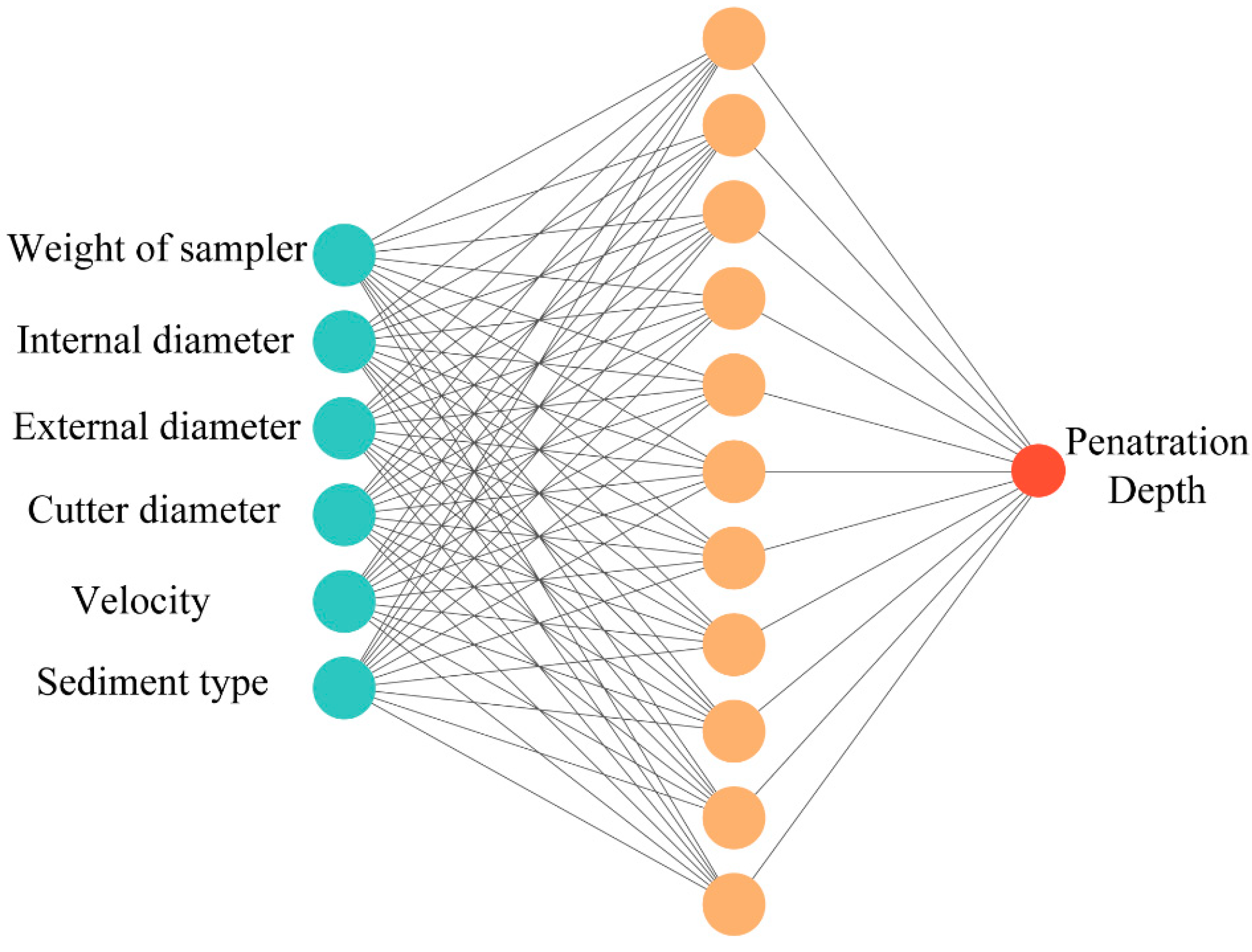
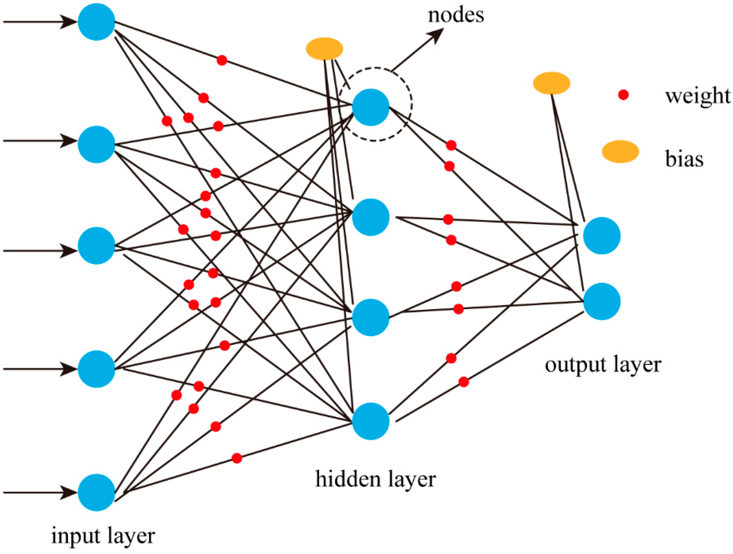
The MLP (multilayer perceptron, also known as artificial neural network) [27] is a simplified biological model that mimics signal propagation in biological nerves and is also one of the most widely used and studied neural network models. It is also called feedforward (Figure 1) because the information flows through a function of x, through an intermediate computational process used to define f, and finally to the output, y. There is no feedback connection between the output of the model and the model itself. When feedforward neural networks are extended to include feedback connections, they are called recurrent neural networks. MLP consists of a multilayer neural network in which the input and output layers consist of a single-layer network. The hidden layer can be a single layer or a multi-layer network, and each layer consists of multiple neurons. Each neural network consists of multiple neurons, each neuron is a perceptron, the neurons in each layer are interconnected, and the connections are fully connected. In a nutshell, the structure of a BP neural network [28] is that the input layers receives a stimulus and passes it to the hidden layers. The output layers compare the results. Suppose the output layer compares the results and is not correct. In that case, it returns to modify the weights of neuron interconnections, also known as the feedforward multilayer network algorithm trained according to the error backpropagation method. Although a large number of new machine learning algorithms have been created, the backpropagation method of BP neural networks is the basis for the vast majority of model training.

A feedforward neural network is mathematically represented as:

$$y_k\left(x\right)={\displaystyle \sum }_{i=1}^M{\omega }_{ih}\times T_r\left(Z\right)+b_{ih}$$

(1)

$$z={\displaystyle \sum }_{i=1}^D{\omega }_{ho}\times X_i+b_{ho}$$

(2)

where x is the input parameter; ${\omega }_{ih}$ and ${\omega }_{ho}$ are the weights from input-layer to hidden-layer and weights from hidden-layer to output-layer, respectively; $b_{ih}$ and $b_{ho}$ are the deviation parameters; M is the number of nodes in the hidden layer; d is the number of nodes in the input layer; and $T_r\left(Z\right)$ is the transfer function that performs a nonlinear transformation of the summation input.

The objective of the algorithm is to reduce the error between the computed value and the actual value through a training series, and the error E can be defined as:

$$E=\frac{1}{p}{\displaystyle \sum }_{p=1}^p{E}_p$$

(3)

where p is the total number of training patterns, and Ep is the error of the p-th training pattern obtained from the following equation:

$$E_p=\frac{1}{2}{\displaystyle \sum }_{k=0}^N{\left(O_k-t_k\right)}^2$$

(4)

where N is the total number of output nodes, k is the output of the k-th output node, and t_k is the target output of the k-th output node.

After each error is calculated, feedback is propagated forward. The weight values are updated to bring the network closer to the actual expression values until all training data are trained. A set of training data is usually trained several times; each training is called a generation (Epoch), and generally, the training stops when the set parameter conditions are reached.

3. Application and Analysis

In this section, we describe the gravity sampling penetration depth dataset used for modeling and the specific process of modeling. The study was performed with scikit-learn, an open-source machine learning package, using Windows 10 64-bit on a CPU with AMD Ryzen 3700x, GPU NVIDIA GeForce RTX 3080, and 16GB of RAM.

3.1. Data Description

The data used in this paper consist of two parts: the measured data from the actual sampling at sea and the physical simulation data obtained from the gravity sampler model tests. The data measured at sea were obtained from several marine geological survey projects in Guangzhou from 2006 to 2011 [8], as well as an investigation cruise of the First Institute of Oceanography of the State Oceanic Administration [10] with 19 datasets. Du [11] obtained the physical simulation data in 2014 through an isometric reduced-gravity sampler experiment with a total of 56 datasets. The data measured at sea mainly include sampler mass, sampling tube inner and outer diameter, cutterhead diameter, and sediment description. The physical simulation data mainly include sampler mass, penetration velocity, sampler inner and outer diameter, cutter head diameter, sediment type, etc. The data include datasets from different deep-sea study areas with deep sampling depths and physical model sampling datasets with shallow sampling depths. Modeling with datasets with a wide range of data can indicate the generalizability of the present model to the gravity sampling problem.

3.2. Prediction Performance Metrics

The performance of the machine learning model was evaluated using the following statistical metrics: explained variance score (EVS), mean absolute error (MAE), mean square error (MSE), and the determination coefficient (R²). The value of EVS is in the range of [0, 1]. Values closer to 1 mean that the independent variable can explain the dependent variable of the variance, and the lower the value, the worse the effect. MAE is used to assess the degree of closeness between the prediction results and the real dataset, and a lower value indicates a better fit. MSE is the mean of the errors of the fitted data and the original data corresponding to the sample points, and the lower the value, the better the fit. R² is the variance score of the explanatory regression model, and its value ranges from [0, 1]. Values closer to 1 mean that the independent variable can explain the variance change of the dependent variable, and lower values mean that the effect is worse. The mathematical expressions of the performance metrics are as follows:

$$EVS=1-\frac{Var\left\{y\_p-y\_t\right\}}{Var\left\{y\_p\right\}}$$

(5)

where y_p is the predicted output; y is the true target output; and Var is variance, the square of the standard deviation.

$$\mathit{MAE}=\frac{1}{n_{\mathrm{samples}}}{\displaystyle \sum }_{i=0}^{n_{\mathrm{samples}}-1}\left|yi\_t-yi\_p\right|$$

(6)

where yi_p is the predicted value of the i-th sample, and yi_t is the corresponding true value.

$$\mathit{MSE}=\frac{1}{n_{\mathrm{samples}}}{\displaystyle \sum }_{i=0}^{n_{\mathrm{samples}}-1}{(yi\_t-yi\_p)}^2$$

(7)

where yi_p is the predicted value of the i-th sample, and yi_t is the corresponding true value.

$$R^2=1-\frac{{{\displaystyle \sum }}_{i=1}^n{(yi\_t-yi\_p)}^2}{{{\displaystyle \sum }}_{i=1}^n{(yi\_t-\overline{y})}^2}$$

(8)

where yi_p is the predicted value of the i-th sample, and yi_t is the corresponding true value. For n total samples, $\overline{y}=\frac{1}{n}{\displaystyle \sum }_{i=1}^{n}yi\_t$ and ${\displaystyle \sum }_{i=1}^n{(yi\_t-yi\_p)}^2={\displaystyle \sum }_{i=1}^n{ϵ}_i^2$.

3.3. Neural Network

3.3.1. Input Layer and Output Layer

In the paper from which the above data were derived, the authors also used seawater density, gravitational acceleration, sampler density, drag coefficient, and friction coefficient to calculate the penetration depth. However, it is clear from the analysis that parameters such as seawater density, gravitational acceleration, and sampler density are essentially constant between samplers (considering that gravity piston samplers are made of steel and lead), and the friction coefficients reported in the original article were derived by extrapolation from the type of sediment. Therefore, in this paper, the six parameters of weight of sampler, internal diameter, external diameter, cutter diameter, velocity, and sediment type are selected as input parameters of the neural network (

Table 1. Input parameters for gravity corer penetration depth.

Parameter	Range
Weight of sampler (kg)	20–2230
Internal diameter (m)	0.042–0.1
External diameter (m)	0.058–0.127
Cutter diameter (m)	0.072–0.1411
Velocity (m/s)	2.8–14.0561
Sediment type	Clay = 1; Silt = 2; Fine Sand = 3; Sand = 4

). Sediment type numbers are expressed only from smallest to largest based on particle size; other representations are also acceptable. The output layer parameter is undoubtedly the penetration depth of the gravity sampler.

3.3.2. Data Preprocessing

First, the data are sorted and organized according to the input layer parameters determined in step (1). A total of 75 sets are obtained; each dataset includes six calculated parameters and one actual penetration depth. The data were randomly disordered, and the train set and the test set were divided in a ratio of 65%: 35%. Thus, a training set containing 48 groups of data and a test set containing 27 groups were obtained.

In the modeling of machine learning, when the values of various parameters have a large quantitative difference in the accuracy of the training results, inaccurate prediction models can easily result. To make model predictions more accurate, it is often necessary to convert data from different specifications to a uniform specification or from other distributions to a specific distribution, collectively referred to as “dimensionless” data. Standard processing methods include min–max scaling and standardization scaling. Min–max scaling can converge the data to the range of [0, 1], and it can project the data to a normal distribution with a mean of 0 and a variance of 1 according to the normal distribution. StandardScaler is chosen for feature scaling in most machine learning algorithms because MinMaxScaler is very sensitive to outliers. Therefore, in this paper, StandardScaler is chosen to preprocess the data.

3.3.3. Hidden Layer

The number of layers and nodes of hidden layers is significant in constructing neural networks. So far, no study has been able to arrive at the optimal number of hidden layers and nodes for a research problem. Therefore, when constructing neural networks for specific issues, it is necessary to try to obtain a more optimal network based on the parameters of the actual data. Therefore, 30 gravity sampling depth prediction models are constructed by varying the number of hidden layers from 1 to 30, with other conditions and model parameters unchanged. The four model accuracy check parameters mentioned in Section 3.2 are used for evaluation, and the best model is selected after a comprehensive comparison.

To choose the most suitable number of hidden layer nodes, it is necessary to consider the accuracy of the model prediction results and the increase in computational cost caused by the rise in the number of hidden layer nodes. Therefore, a model with high accuracy and low computational cost is desirable. In terms of model prediction accuracy, the results can be seen in Figure 2. All four evaluation methods show the same trend. With the increase in the number of hidden layer nodes, the accuracy increases first, suddenly decreases at the position of node number 7, continues to increase, suddenly increases to number 8, and has a small up and down oscillation before number 11, with no more significant changes. Therefore, the model is accurate enough with 11 hidden layer nodes. On the other hand, the lower the number of nodes, the more efficient the prediction model is in terms of computational cost. Considering the above two influencing factors, the prediction models of sampler penetration depth with a number of nodes ranging from 11 to 15 are all acceptable. The model calculation accuracy does not differ much, and the efficiency is good. We chose 11 as the number of nodes in the hidden layer in this study, and other numbers of nodes are also acceptable.

Finally, a gravity sampler penetration depth machine learning model (Figure 3) was built with six parameters consisting of weight of sampler, internal diameter, external diameter, cutter diameter, velocity, and sediment type as the input layer; 11 nodes as the hidden layer; and penetration depth as the output layer. A final gravity sampling penetration depth prediction model can be made by using this structured neural network to train and test the gravity sampling data.

4. Results

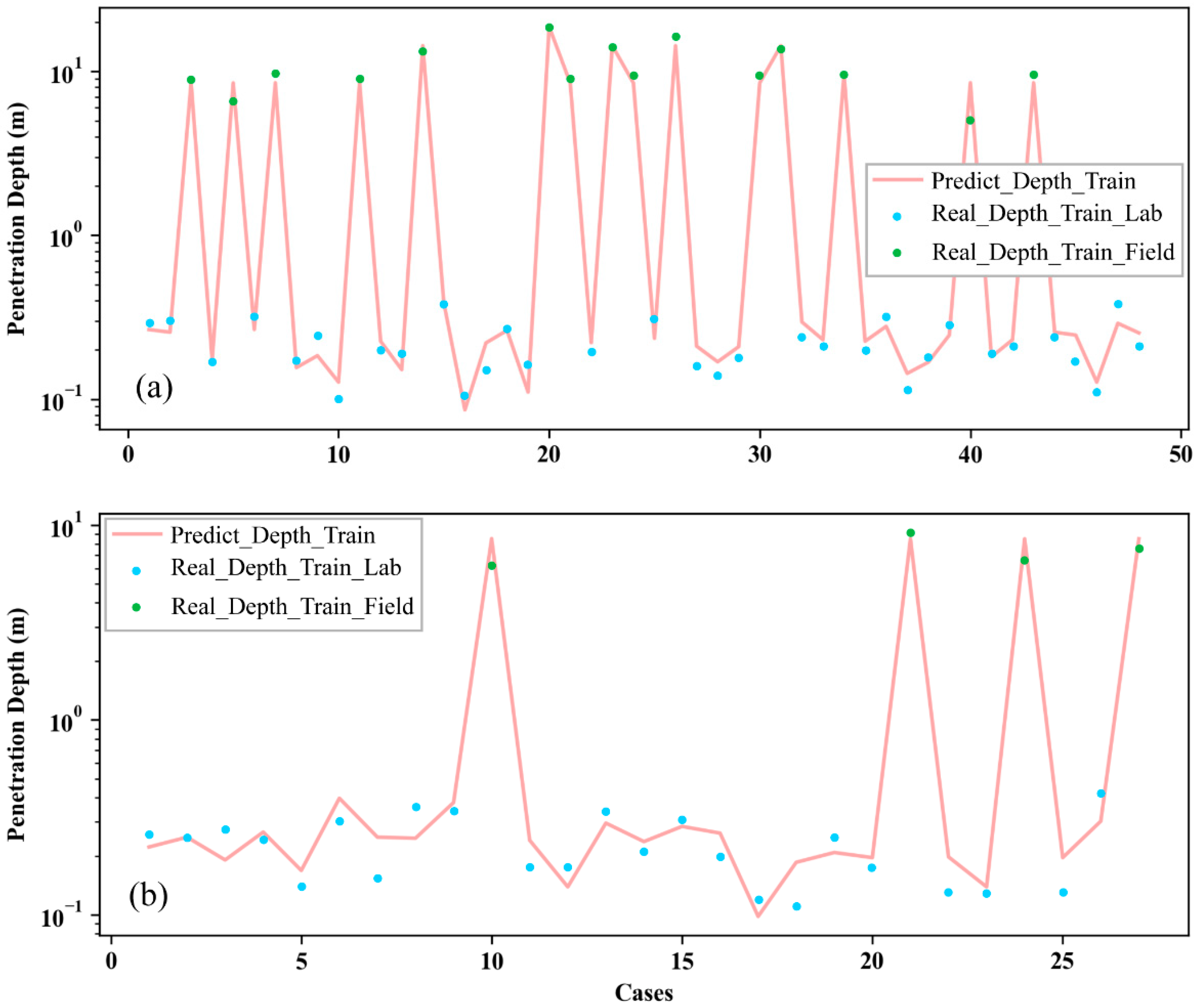
Figure 4 shows the gravity sampler penetration depth prediction results using the training and test sets of the established machine learning model. The results predicted by the model are in good agreement with the actual results in both the training and test sets. As shown in Figure 5, the prediction error is small, despite the significant difference in gravity sampler parameters between the data measured at sea and the physical model tests. The prediction accuracy statistics of the train and test sets are shown in

Table 2. Prediction accuracy statistics of train set and test set.

	EVS a	MAE b	MSE c	R2
Trian set	0.98	0.34	0.56	0.98
Test set	0.95	0.26	0.38	0.94

^a EVS is explained variance score; ^b MAE is mean absolute error; ^c MSE is mean square error.

. Both datasets showed promising results on all four statistical scales, and the training set results are slightly better than those of the test set.

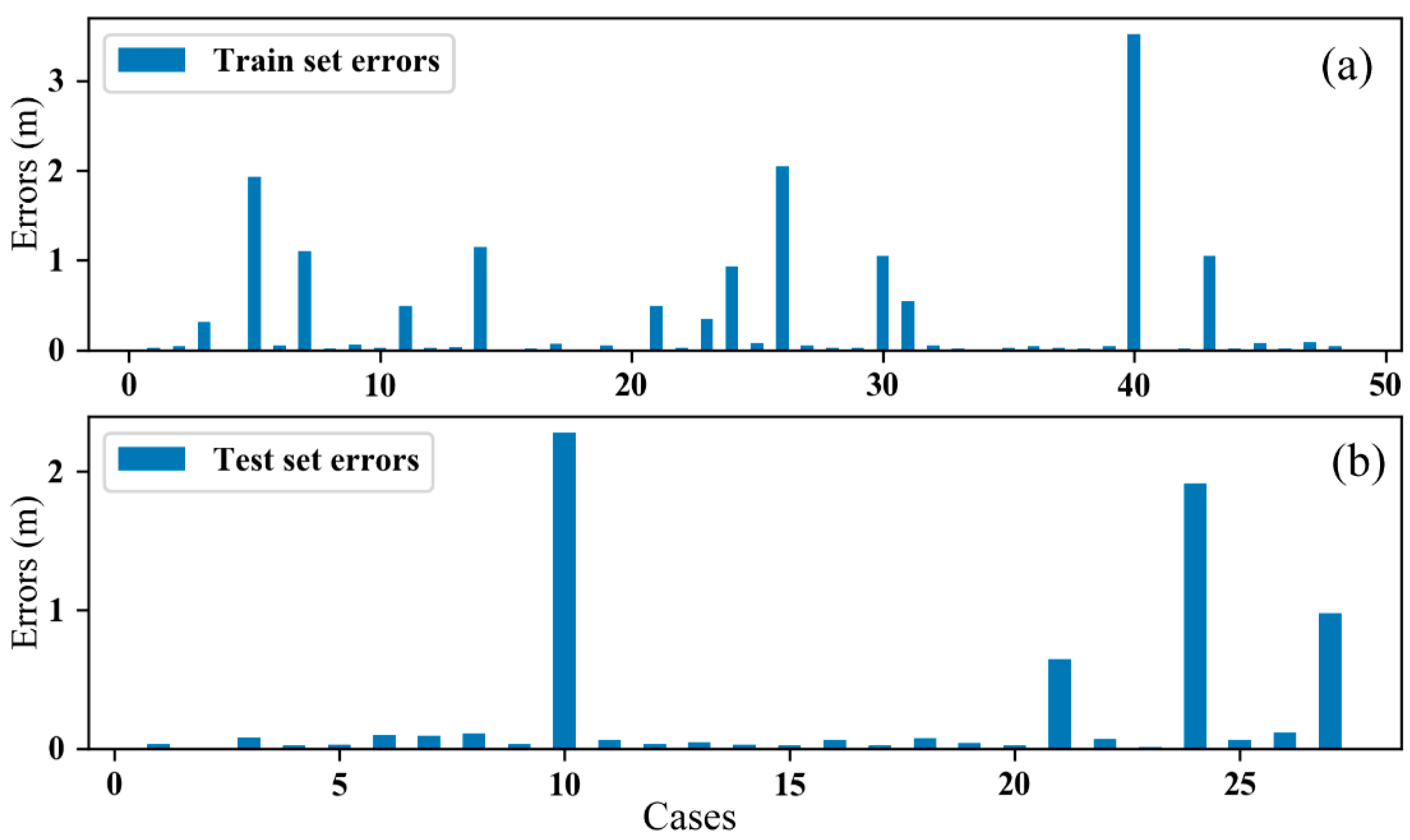
The absolute values of the error between predicted and real penetration depth are shown in Figure 4. The training set error of most cases is less than 1 m. There are six cases with error values between 1 and 2 m and one case with an error more than 3 m in the train set. As for the test set, 23 cases of 27 are less than 0.5 m, and there are only 2 cases with errors over 1 m. Many factors affect the penetration depth of gravity sampling (geology, marine environment, seafloor topography, etc.). Even if the same sampler is used under the same geological conditions, the depth of each sample is not the same, and the error can reach 2~3 m [9]. Therefore, numerical model prediction results within 2~3 m are acceptable. The machine learning model used in the paper is exceptionally accurate, as most errors are less than 1 m.

After analyzing the data, we found that the 18 examples with large error values were all data measured at sea. There are two main reasons for this situation: (1) the amount of data of the same type and (2) the error of the data itself. When there are only 19 actual at-sea data point with a slight difference in sampler quality and 56 physical model test data, the model will tend toward the accuracy of the physical model test. Another reason is that human operation and recording errors of at-sea sampling are more significant than those in physical model tests. The high value of the prediction error for the offshore sampling depth is due to the typical machine learning model training problem caused by the relatively small amount of offshore sampling data. In the training process of machine learning models, the accuracy of the model can be increased when the training data sample is large enough. When the training data sample is insufficient, errors tend to be increased. The training data used in this paper are limited due to the difficulty of obtaining data for ocean gravity sampling. The model prediction error will decrease with increased offshore gravity sampling penetration depth data.

5. Discussion

5.1. Accuracy and Applicability of Machine Learning Model

Machine learning has different characteristics when applied in different fields, and there are many factors that affect the accuracy of machine learning. When machine learning is applied to the field of marine geology, several main factors affect the prediction accuracy:

(1)

Whether the geological problem is suitable for machine learning models;

Although machine learning models can be applied to many problems, they still cannot solve all problems. Machine learning methods are suitable for solving problems that can be accurately calculated quantitatively; have a large amount of accurate associated research data; and require experience, such as geohazard prediction, weather forecasting, geological phenomenon identification, etc. Some geological problems that do not have associated data or for which the amount of data does not meet machine learning requirements, such as tectonic geology and geological hazard on-site monitoring, are not suitable for machine learning solutions.

(2)

Whether the selected input factors are complete and representative of the entire geological process;

Due to their complexity, geological problems are often subjected to various internal and external geodynamic effects. For example, there may be more than a dozen factors influencing the evaluation of submarine landslide hazards. However, we do not need to bring all the influencing factors into the model for calculation because there is a specific correlation between many influencing factors (such as wind speed and waves). In addition, having too many influencing factors is not conducive to modeling efficiency. Therefore, when we choose the input parameters of the machine learning model, we need to select several factors with the most significant degree of influence through professional knowledge analysis. Having too many chosen factors is not conducive to data acquisition and modeling efficiency, and having too few factors is not representative of the geologic process.

(3)

The quality and quantity of the data;

The core objective of machine learning is to obtain the desired patterns from a large amount of available data through numerical methods. Therefore, the quality and quantity of the data itself are essential. When machine learning is applied in data-rich fields, such as the Internet and finance, the amount of data generated per second is several Gs, so there is no data volume problem. However, the geological field does not have a large amount of data related to many issues due to the difficulty and high cost of obtaining data, which are the main reasons for some errors in model prediction results. Like the gravity sampler penetration depth problem studied in this paper, there are only 19 groups of real sampling data from the seafloor. Each data group contains a certain amount of human and environmental errors, so it is challenging to represent the sampling penetration process accurately through the data. Therefore, there must be relative error values in the prediction results.

(4)

Whether an appropriate machine learning model has been selected to solve the geological problem;

Different machine learning methods can solve the same geological problem, and it is essential to choose a suitable algorithm. Even if the research problem is identified as a specific category of regression, fitting, clustering, etc., each category has multiple algorithms. Furthermore, new machine learning models are being developed all the time.. When it is impossible to determine which algorithm is suitable for a geological problem, more than one should be tried. The appropriate algorithm should be selected through analysis and comparison. In addition, there is no best algorithm—only the algorithm that meets the accuracy needs of the research problem through data, algorithm selection, and model training.

5.2. Comparison of Different Penetration Depth Models

To demonstrate the accuracy of the gravity sampler penetration depth machine learning model developed in this paper, three other t analytic solution models, defined as AS1 [9], AS2 [11], and AS3 [10], were used for computation and comparison. The 75 groups of gravity sampling data analyzed in this paper were computed using machine learning models and three other analytical solution models. The penetration depths calculated by the four models were analyzed in comparison to the actual penetration depths obtained using statistical methods (MSE, MAE, EVS, and R²) mentioned in Section 3.2.

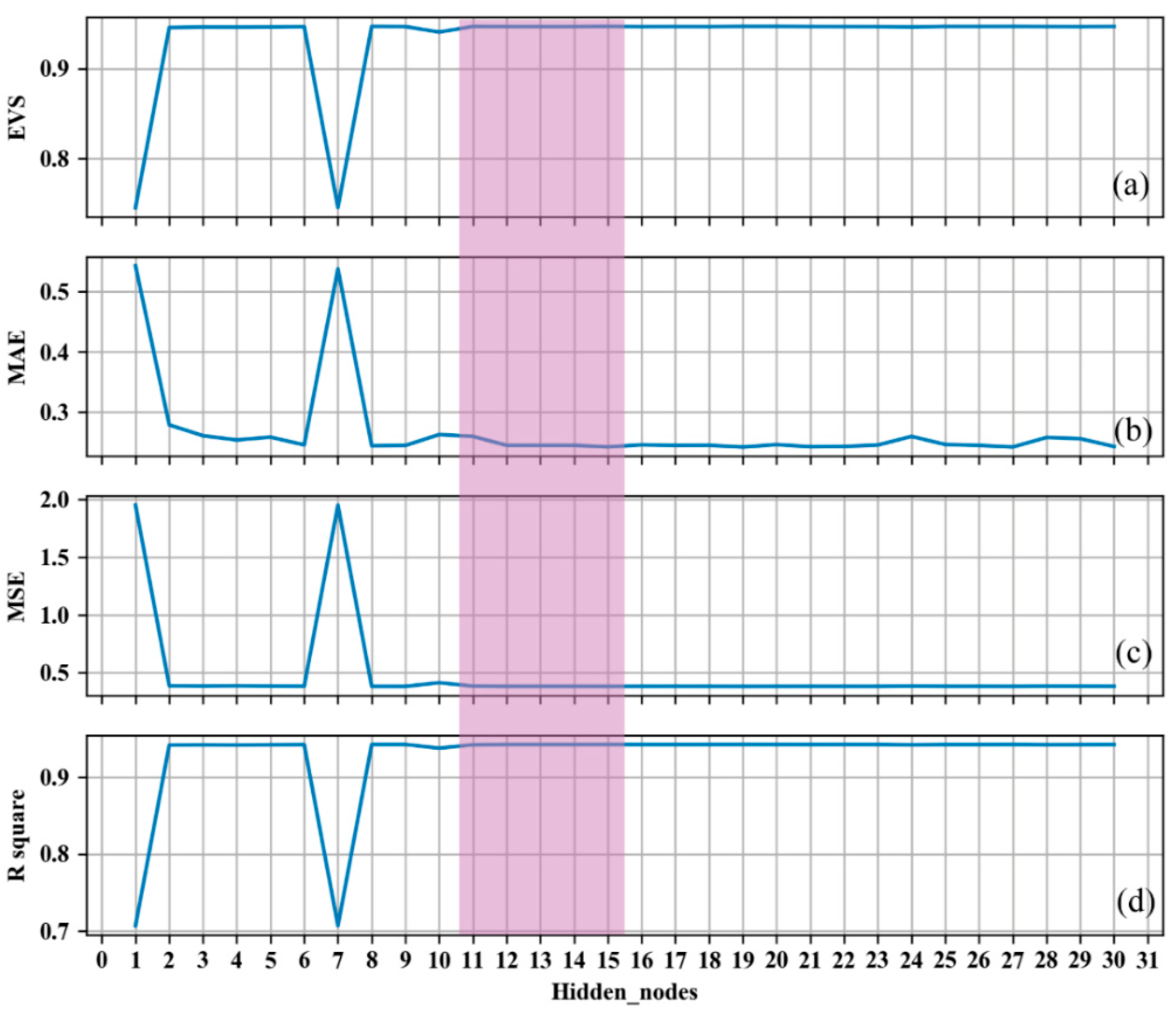
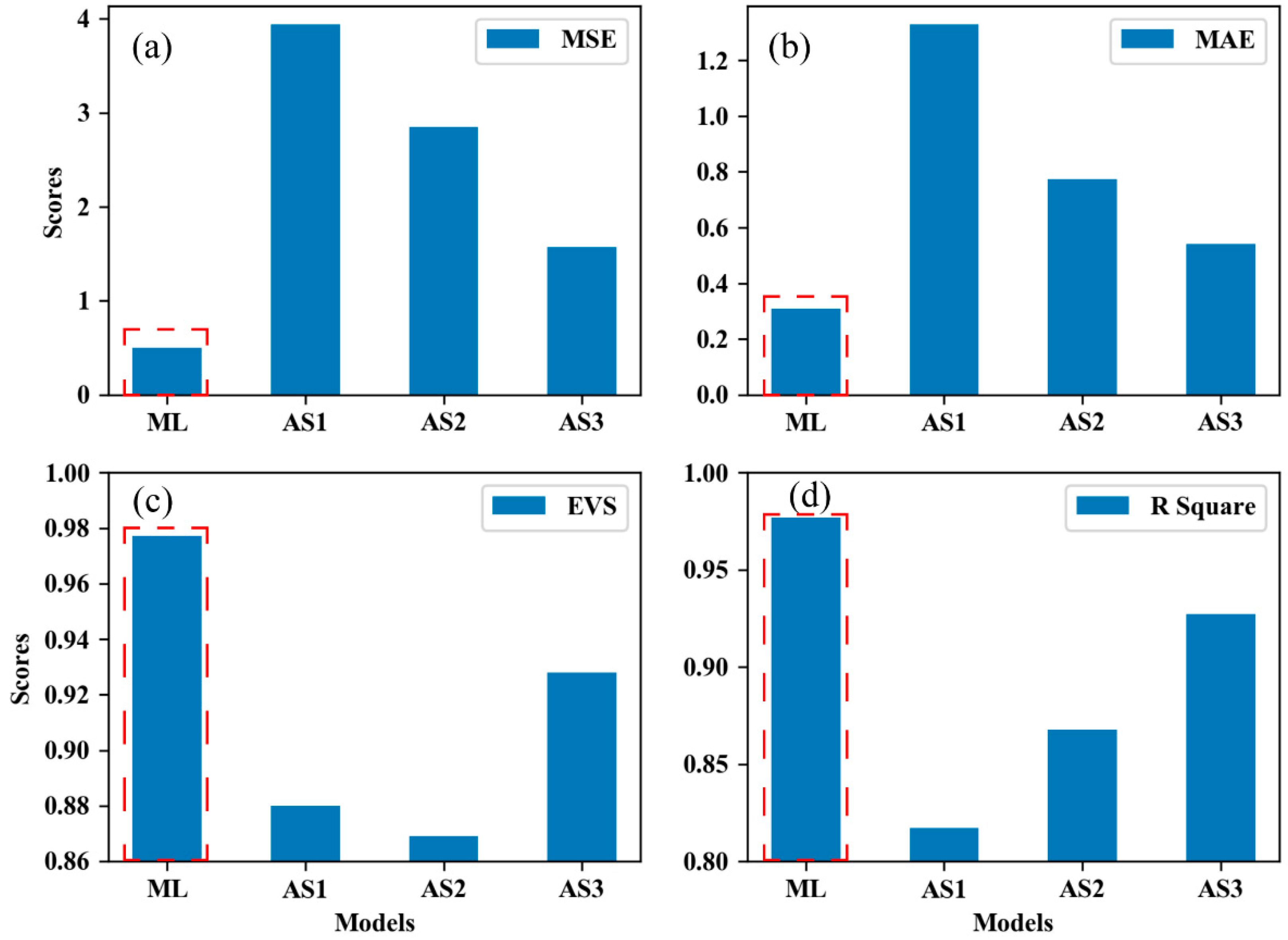
The comparison results of the accuracy of different gravity sampling penetration depth prediction models are demonstrated in

Table 3. Statistical performance metrics of different penetration depth models.

Model	Performance Metrics
	MSE	MAE	EVS	R2
ML	0.50	0.31	0.98	0.98
AS1	3.94	1.33	0.88	0.82
AS2	2.85	0.77	0.87	0.97
AS3	1.57	0.54	0.93	0.93

Note: MSE = mean square error; MAE = mean absolute error; EVS = explained variance score; R² = determination coefficient. Underline denotes the best performance value for each performance metric.

and Figure 6. It well known that smaller MSE and MAE and larger EVS and R² values indicate more accurate prediction results. In terms of statistical metrics, the ML model yields the lowest MSE and MAE and the highest EVS and R² values. As for the other three analytic solution models, AS3 performs best on MSE, MAE, and EVS, and AS2 performs best on R². Therefore, the accuracy of the four models is: ML > AS3 > AS2 > AS1. Moreover, the performance of the machine learning model is clearly and substantially ahead of that of the other analytical solution models.

The prediction accuracy of machine learning models is much higher than that of various analytical solution models because the two computational methods employ very different processes. The traditional analytical solution model mainly analyzes the force of the gravity sampler penetration process, derives the energy of each component and process, and solves the equation according to energy conservation. This way of solving the energy conservation equation presents the following problems: (1) the calculation of each process is approximated, leading to the existence of certain errors; (2) there is a certain abbreviation in the calculation process, for example, AS2 does not consider the cutter head cutting work; and (3) because it involves sliding friction work between the sampling tube and the sediment, cutting work, and other processes, the calculation requires the estimation and approximation of the friction coefficient and other parameters, so it is difficult to calculate accurately. The machine learning model only needs to establish the numerical relationship between the input parameters and the penetration depth directly through continuous training and backpropagation based on the data, skipping the complex and extensive approximation process of various forces and energy calculations. Therefore, the prediction results of machine learning models are more accurate.

In addition, because solving the energy conservation equation contains the physical meaning of numerous sampler penetration processes, many process parameters are required, such as the inner wall friction coefficient, outer wall friction coefficient, cutter head cutting coefficient, and other difficult-to-determine parameters. This status quo leads to numerous estimates for the modeling of the conventional analytical solution, which increases the complexity of the computational process and the error of the prediction results. In contrast, the machine learning model only requires a few critical influencing parameters to directly connect with the penetration depth. The computational parameters used in this model can be obtained before sampling. No parameter valuation is required, which significantly reduces the complexity of the model calculation and improves the prediction accuracy. Overall, the machine learning algorithm is superior to traditional analytical solution models in predicting the penetration depth of gravity samplers, both in terms of the accuracy of the model prediction results and the scientific nature of the computational process.

6. Conclusions

In this study, a machine learning model using an MLP neural network was applied to predict the penetration depth of a gravity corer. A database of 75 gravity corer penetration depths from both real sampling at sea and physical model test data was used to generate the datasets for modeling, considering six penetration depth factors. The models were validated using the MSE, MAE, EVS, and R-square methods. The results show that the proposed machine learning model achieved great accuracy in predicting the gravity corer penetration depth (test set accuracy: EVS = 0.95, MAE = 0.26, MSE = 0.38, R² = 0.94). Furthermore, in this study, we used three analytical solution models of gravity corer penetration depth to predict the same cases. The results show that the machine learning model is superior to the traditional analytical solution models in terms of both the accuracy of the prediction results and the scientific nature of the computational process. Thus, it can be reasonably concluded that the proposed machine learning model can be used to achieve better penetration depth prediction. However, many factors affect the accuracy of the machine learning model: problem type, selection of influential factors, quality and quantity of data, and selection of machine learning models. Therefore, it is better to collect more high-quality data and select a moderate machine learning model and influential factors to obtain a more accurate machine learning model.

References

1. Kullenberg, B. Piston Core-Sampler. Nature 1947, 160, 410. [Google Scholar] [CrossRef]
2. Zhang, X.; Luan, Z.; Yan, J.; Chen, C.A. A Review of Development in Deep-sea Long Coring System. Mar. Geol. Front. 2012, 28, 40–45. [Google Scholar] [CrossRef]
3. Chen, Z.B.; Yang, G.; Wu, Y.H. Application of Long Gravity Piston Corer in the Okhotsk Sea. Adv. Mar. Sci. 2013, 31, 553–558. [Google Scholar] [CrossRef]
4. Sansone, F.J.; Hollobaugh, J.T. Diver-Operated Piston Corer for Nearshore Use. Estuaries 1994, 17, 716–720. [Google Scholar] [CrossRef]
5. Zolitschka, B.; Francus, P.; Ojala, A.E.K.; Schimmelmann, A. Varves in lake sediments—A review. Quat. Sci. Rev. 2015, 117, 1–41. [Google Scholar] [CrossRef]
6. Zhu, H.Y.; Liu, Q.Y.; Wang, G.R.; Yu, Z.Y.; Jiang, Z.L.; Zhong, Y.S. Research status and development of natural gas hydrate sampling device. Nat. Gas Ind. 2009, 29, 63–66. [Google Scholar] [CrossRef]
7. Luan, X.; Yue, B.; Obzhirov, A. Sea Floor Topography of Shallow Gas Hydrate Area: Data from Okhotsk Sea. Geoscience 2008, 22, 420–429. [Google Scholar] [CrossRef]
8. Chen, J.; Fan, W.; Bingham, B.; Chen, Y.; Gu, L.; Li, S. A Long Gravity-Piston Corer Developed for Seafloor Gas Hydrate Coring Utilizing an In Situ Pressure-Retained Method. Energies 2013, 6, 3353–3372. [Google Scholar] [CrossRef] [Green Version]
9. Du, X.; Sun, Y.F.; Hu, G.H.; Song, Y.P. Study of penetration depth of gravity piston corer. Ocean. Eng. 2016, 34, 134–139. [Google Scholar] [CrossRef]
10. Li, M.G.; Wang, T.H.; Cheng, Z.B.; Liu, S.N.; Lin, Q.Q.; Liu, X.; Zhao, J. Analysis Influencing Factors of Deep-Sea Gravity Piston Corer Penetration Depth. Period. Ocean. Univ. China 2013, 43, 94–98. [Google Scholar] [CrossRef]
11. Du, X.; Sun, Y.F.; Song, Y.P.; Zhou, Q.Q.; Jiao, P.F. Study of Penetration Depth from a Model of Gravity Piston Corer. Adv. Mar. Sci. 2018, 36, 88–97. [Google Scholar] [CrossRef]
12. Ren, Y.; Liu, Y.; Ding, Z.; Liu, B.; Zhang, J. Design of Full-Ocean-Depth Self-Floating Sampler and Analysis of Factors Affecting Core Penetration Depth. J. Ocean Univ. China 2020, 19, 1094–1102. [Google Scholar] [CrossRef]
13. Wu, H.; Liu, N.; Peng, J.; Ge, Y.; Kong, B. Analysis and modeling on coring process of deep-sea gravity piston corer. J. Eng. 2020, 2020, 900–905. [Google Scholar] [CrossRef]
14. Lary, D.J.; Alavi, A.H.; Gandomi, A.H.; Walker, A.L. Machine learning in geosciences and remote sensing. Geosci. Front. 2016, 7, 3–10. [Google Scholar] [CrossRef] [Green Version]
15. Khosravikia, F.; Clayton, P. Machine learning in ground motion prediction. Comput. Geosci. 2021, 148, 104700. [Google Scholar] [CrossRef]
16. Chen, J.; Takeyama, T.; O-Tani, H.; Fujita, K.; Hori, M. A Framework for Assessing Liquefaction Hazard for Urban Areas Based on Soil Dynamics. Int. J. Comp. Methods 2016, 13, 1641011. [Google Scholar] [CrossRef]
17. Erzin, Y.; Ecemis, N. The use of neural networks for CPT-based liquefaction screening. Bull. Eng. Geol. Environ. 2015, 74, 103–116. [Google Scholar] [CrossRef] [Green Version]
18. Marjanovic, M.; Bajat, B.; Kovacevic, M. Landslide Susceptibility Assessment with Machine Learning Algorithms. In Proceedings of the International Conference on Intelligent Networking & Collaborative Systems, IEEE, Barcelona, Spain, 4–6 November 2009. [Google Scholar] [CrossRef]
19. Pham, B.T.; Prakash, I.; Bui, D.T. Spatial prediction of landslides using a hybrid machine learning approach based on Random Subspace and Classification and Regression Trees. Geomorphology 2018, 303, 256–270. [Google Scholar] [CrossRef]
20. Qi, C.; Tang, X. Slope stability prediction using integrated metaheuristic and machine learning approaches: A comparative study. Comput. Ind. Eng. 2018, 118, 112–122. [Google Scholar] [CrossRef]
21. Li, P.L.; Tian, W.P.; Li, J.C. The Application of BP Neural Network in the Research of the Landslide Stability. Adv. Mater. Res. 2012, 594–597, 2290–2295. [Google Scholar] [CrossRef]
22. Zolfaghari, Z.; Mosaddeghi, M.R.; Ayoubi, S. ANN-based pedotransfer and soil spatial prediction functions for predicting Atterberg consistency limits and indices from easily available properties at the watershed scale in western Iran. Soil Use Manag. 2015, 31, 142–154. [Google Scholar] [CrossRef]
23. Azadmard, B.; Mosaddeghi, M.R.; Ayoubi, S.; Chavoshi, E.; Raoof, M. Estimation of near-saturated soil hydraulic properties using hybrid genetic algorithm-artificial neural network. Ecohydrol. Hydrobiol. 2019, 20, 437–449. [Google Scholar] [CrossRef]
24. Lawson, E.; Smith, D.; Sofge, D.; Elmore, P.; Petry, F. Decision forests for machine learning classification of large, noisy seafloor feature sets. Comput. Geosci. 2017, 99, 116–124. [Google Scholar] [CrossRef]
25. Song, Y.; He, B.; Liu, P.; Yan, T. Side scan sonar image segmentation and synthesis based on extreme learning machine. Appl. Acoust. 2018, 146, 56–65. [Google Scholar] [CrossRef]
26. Shang, X.; Robert, K.; Misiuk, B.; Mackin-McLaughlin, J.; Zhao, J. Self-adaptive analysis scale determination for terrain features in seafloor substrate classification. Estuar. Coast. Shelf Sci. 2021, 254, 107359. [Google Scholar] [CrossRef]
27. Fausett, L.V. Fundamentals of Neural Networks: Architectures, Algorithms, and Applications; Prentice-Hall, Inc.: Upper Saddle River, NJ, USA, 1993. [Google Scholar]
28. Rumelhart, D.E.; Hinton, G.E.; Williams, R.J. Learning representations by back-propagating errors. Nature 1986, 323, 533–536. [Google Scholar] [CrossRef]
Figure 1. Illustration of a three-layer feedforward neural network.
Applsci 12 04457 g001
Figure 2. Comparison of the accuracy of different hidden-layer node models. The purple area is the relatively appropriate number of hidden layer nodes. (a) Variation of EVS with the increase in hidden nodes; (b) variation of MAE with the increase hidden nodes; (c) variation of MSE with the increase in hidden nodes; (d) variation of R2 with the increase in hidden nodes.
Applsci 12 04457 g002
Figure 3. Illustration of the penetration depth prediction neural network. The green nodes, brown nodes, red nodes represent input node, hidden nodes and output nodes, respectively.
Applsci 12 04457 g003
Figure 4. Comparison of machine learning model predictions with an actual penetration depth of gravity samplers. (a) Comparison of predicted depth values with actual depth values for train data; (b) comparison of predicted depth values with actual depth values for test data. The blue points represent the laboratory data obtained from physical model tests. The green points represent field data obtained from sea.
Applsci 12 04457 g004
Figure 5. The absolute value of the error between predicted and real penetration depths of a gravity corer with machine learning models. The absolute error values were obtained by subtracting the predicted values from the true values and then taking the absolute value. (a) Errors of train set; (b) Errors of the test set.
Applsci 12 04457 g005
Figure 6. Comparison of the accuracy of results from different gravity sampling penetration depth prediction models. (a) Comparison of MSE of prediction results of four models; (b) comparison of MAE of prediction results of four models; (c) comparison of EVS of prediction results of four models; (d) comparison of R2 of prediction results of four models. ML is the machine learning model, AS1 is analytical solution model 1, AS2 is analytical solution model 2, and AS3 is analytical solution model 3. The smaller the value of MSE and MAE, the higher the accuracy. The larger the EVS, the higher the accuracy. The closer R is to 1, the better the prediction result. The red dashed line denotes the best performance value for each performance metric.
Applsci 12 04457 g006