Article

Grouping Bilinear Pooling for Fine-Grained Image Classification

School of Microelectronics, University of Science and Technology of China, Hefei 230026, China
*
Author to whom correspondence should be addressed.
Appl. Sci. 2022, 12(10), 5063; https://doi.org/10.3390/app12105063
Submission received: 11 April 2022 / Revised: 16 May 2022 / Accepted: 16 May 2022 / Published: 17 May 2022
(This article belongs to the Special Issue Recent Advances in Deep Learning for Image Analysis)

Abstract

:
Fine-grained image classification is a challenging computer visual task due to the small interclass variations and large intra-class variations. Extracting expressive feature representation is an effective way to improve the accuracy of fine-grained image classification. Bilinear pooling is a simple and effective high-order feature interaction method. Compared with common pooling methods, bilinear pooling can obtain better feature representation by capturing complex associations between high-order features. However, the dimensions of bilinear representation are often up to hundreds of thousands or even millions. In order to get compact bilinear representation, we propose grouping bilinear pooling (GBP) for fine-grained image classification in this paper. Firstly, by dividing the feature layers into different groups, and then carrying out intra-group bilinear pooling or inter-group bilinear pooling. The representation captured by GBP can achieve the same accuracy with less than 0.4% parameters compared with full bilinear representation when using the same backbone. This extreme compact representation largely overcomes the high redundancy of the full bilinear representation, the computational cost and storage consumption. Besides, it is because GBP compresses the bilinear representation to the extreme that it can be used with more powerful backbones as a plug-and-play module. The effectiveness of GBP is proved by experiments on the widely used fine-grained recognition datasets CUB and Stanford Cars.

1. Introduction

Computer vision is an important field of artificial intelligence, and its goal is to realize the extension of human vision function based on intelligent computing. Image classification is the most basic task in computer vision. In general, Image classification can be divided into two categories: coarse-grained image classification and fine-grained image classification. Recognizing images of different classes (cats, dogs, flowers, planes, etc.) is the goal of coarse-grained image classification, and fine-grained visual classification aims at classifying sub-classes of category [1,2]. Fine-grained visual classification is a challenging visual task due to the small interclass variations and large intra-class variations. Obtaining more discriminative feature representation is the focus of fine-grained image classification. Convolutional Neural Network (CNN) has been widely used in computer vision tasks [3,4,5]. By stacking different functional layers, CNN can obtain powerful feature extraction and generalization capabilities. Extracting expressive feature representation is an effective way to improve the accuracy of fine-grained image classification; many enlightening and meaningful works are proposed to make better use of the extracted CNN semantic features.
Most studies obtain the feature representation of an input image by pooling high-order features [6,7], extracting high-value information through attention methods [8,9] or aggregating the features of different levels [10], then use these expressive representation to subsequent tasks. In addition, some other studies use the high-order statistical information of features to obtain better feature representation, such as Fisher Vector [11,12], VLAD [13], spatial pyramids [14] and full bilinear pooling [15,16]. Among them, the full bilinear pooling (FBP) [15] captures the complex correlation between paired features and uses the bilinear representation for classification which makes remarkable achievements in fine-grained image classification. However, the bilinear representation is as high as hundreds of thousands or even millions of dimensions. It is far higher than the aggregating representation obtained by common pooling methods, resulting in huge computational load and memory consumption, and limiting the expansion of the model structure.
In order to reduce the dimension of the bilinear representation and obtain compact representation, refs. [16,17,18,19,20] simplify the bilinear pooling in different ways. In [17], the image classification network based on bilinear pooling is regarded as a linear kernel machine, and it is proved that bilinear pooling enables the linear classifier to have the recognition ability of second-order kernel machine. Then, Random Maclaurin (RM) [21] and Tenor Sketch (TS) [22] are used for low-dimensional approximation, and a compact bilinear pooling (CBP) is established. Ref. [18] uses the Hadamard product instead of bilinear pooling, the Hadamard product also achieves a low-dimensional approximation to bilinear pooling. Refs. [16,19] reduces the dimensions of representation by carrying out feature mapping on high-order feature layers or simplifying bilinear pooling by matrix factorization to get compact representation. The learnable semantic grouping module is introduced to reduce the computation of bilinear pooling in [20].
Besides, some papers focus on what else compact bilinear pooling can do [23,24,25,26]. Ref. [23] uses multimodal compact bilinear pooling in visual question answering which performs well. In [24], bilinear pooling is used to combine global features and local features for person re-identification. Ref. [25] aggregates local CNN features by carrying out bilinear pooling to obtain 3D object representation and achieves remarkable results in 3D object recognition tasks. In [26], bilinear blocks are proposed to obtain rich modality-temporal representation for RGB-D Action Recognition.
Bilinear pooling has potential in different visual tasks. Inspired by various compact bilinear pooling methods, we want to simplify bilinear pooling in a simple way and compress the bilinear representation to the extreme. We first re-analyze bilinear pooling in Section 2, it is shown intuitively that the bilinear representation is actually a low-rank self-correlation and cross-correlation representation. Then, the reason for high redundancy of bilinear representation is analyzed. To compress the bilinear representation to the extreme, we propose grouping bilinear pooling (GBP) to minimize the dimensions of bilinear representation. Comparing with different compact bilinear pooling methods, GBP reaches the best accuracy with the fewest parameters. In addition, GBP can be embedded into different models as a plug-and-play module and can achieve a competitive performance compared with other state-of-the-art approaches. Experiments on the CUB-200-2011 [1] dataset and the Stanford Cars [2] dataset show the effectiveness of GBP.

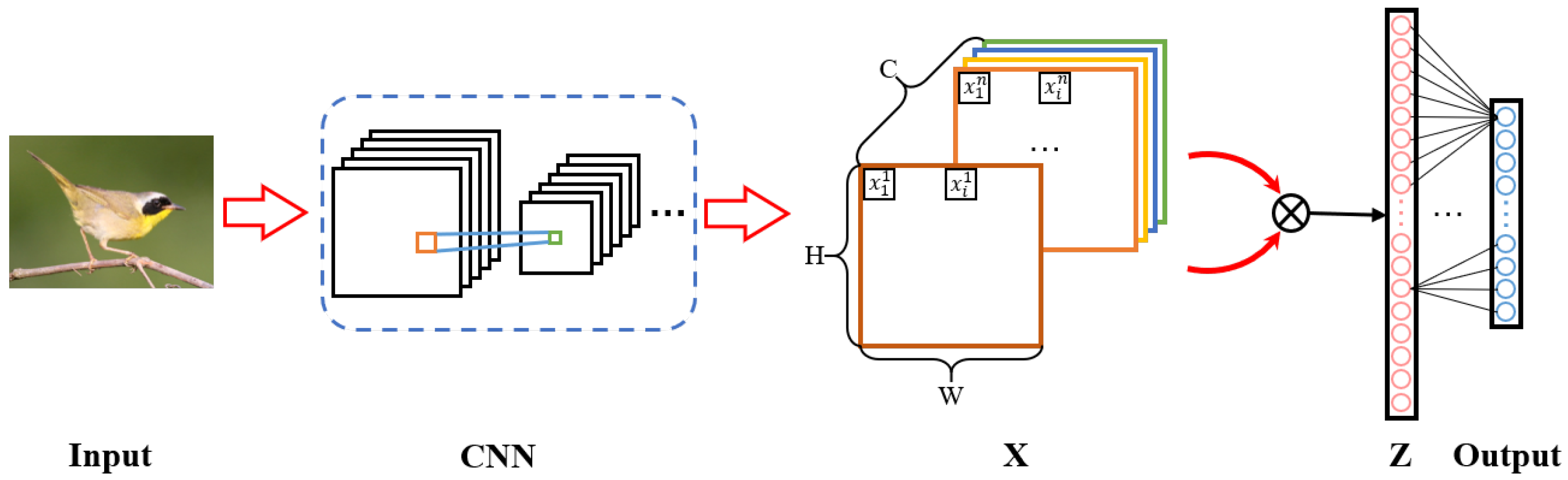
2. Analysis of Bilinear Pooling

In BCNN [15], in order to get the full bilinear representation Z of the input image, CNN is used to extract the higher-order feature representation X of the input image, X R C × H × W , where C is the number of feature layers, H and W are the height and the width of feature layers, respectively. For each feature layer, there are H × W different locations. The architecture of BCNN is illustrated in Figure 1.
Here, we define local descriptor x i T = x i 1 , x i 2 , , x i C R C ( i [ 1 , , H W ] ) , x i n represents the value of ith position on the n t h feature layer. Besides, for convenience, considering x i as a vector the dimension of which is C. The bilinear representation Z is as follows:
Z = 1 H W i H W x i x i T = 1 H W i H W x i 1 x i 1 i H W x i 1 x i C i H W x i 1 x i C i H W x i C x i C .
Vectorizing Z, vector ( Z ) R C 2 . Assuming C is 512, vector ( Z ) will be up to 250 K dimensions. The high dimensions of bilinear representation result in high computation and storage costs.
The representation Z is used for classification after passing through the full-connection layer,
O u t p u t = Z W C + b = 1 H W i H W x i x i T W C + b C ,
where W C R C 2 × N is the weight matrix of the full-connection layer, b C R k , O u t p u t   R N , N is the number of categories. In general, C 2 N , the rank of W C is as follows:
r a n k W C min C 2 , N = N .
Vectorizing the ith feature layer: f i T = x 1 i , x 2 i , , x H W i R H W , F T = f 1 , f 2 , , f C R C ,
Z = 1 H W f 1 T f 1 f 1 T f c f 1 T f c f c T f c = 1 H W F F T .
O u t p u t = Z W C + b = 1 H W F F T W C + b C .
In [17], RM [21] is used to sample the feature layers, then bilinear pooling is carried out. In fact, the representation obtained by [17] is the recombination of part of the element in Z. The representation obtained by [18], using the low-dimensional approximation of Hadamard product, is the elements on the diagonal of Z. This low-rank approximation actually abandons the vast majority of information of Z. The loss of information is inevitable, although the dimensions of representation are reduced.
X contains C different feature layers f; the bilinear representation Z in Equation (1) is a symmetric matrix. The elements on the diagonal of Z are the dot product sum of the corresponding positions of the feature layer itself. The scalar obtained by the point-wise product can be regarded as the pixel-level self-correlation of the feature layer to some extent. Similarly, the elements on the non-diagonal of Z are the dot product sum of the corresponding positions of different feature layers, which can be regarded as the cross-correlation between feature layers.
Since the bilinear representation obtained by bilinear pooling is a correlation representation with extremely high dimensions between high-order feature layers (increasing with the square of the number of feature layers), it will greatly increase the parameters to be learned by the full-connection layers even if there is only a single-layer full-connection layer. Furthermore, nearly half of the calculations in the symmetric matrices Z are repeated; obviously, it greatly reduces computational efficiency and results in redundancy of the model.

3. Grouping Bilinear Pooling

According to Equation (3), the dimension of Z is often up to hundreds of thousands or even millions, far more than the dimension of O u t p u t , hoping that the full-connection layer will establish high-efficient contact and find high value information between Z and O u t p u t is impractical. Minimizing the huge gap of dimensions between Z and O u t p u t is a highly cost-effective way to improve bilinear pooling.
We propose grouping bilinear pooling (GBP) that by grouping the feature layers X and performing intra-group bilinear pooling (Intra-GBP) or inter-group bilinear pooling (Inter-GBP), the information of the original full bilinear representation can be greatly preserved, and extreme compact bilinear feature representation is available. The differences between GBP with other bilinear pooling methods [15,17,19] are shown in Figure 2, and detailed comparisons are described in the experimental section.

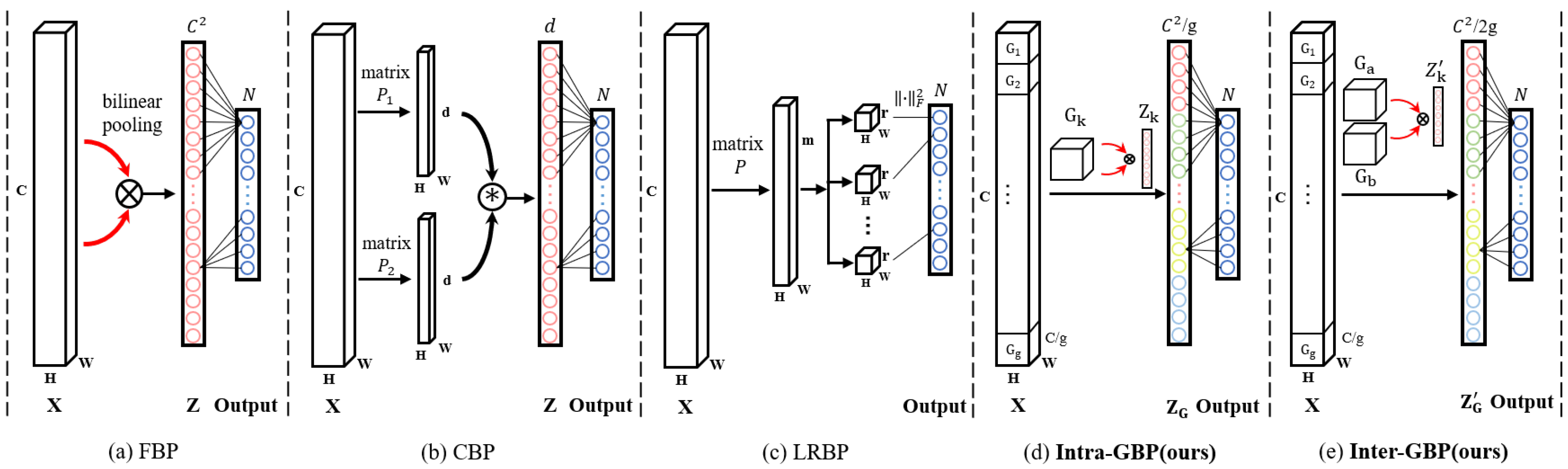
3.1. Intra-Group Bilinear Pooling

Define F is the high-order feature, F T = f 1 , f 2 , , f C , F k R C g , F contains C different feature layers. Then, dividing F into g groups. Noting that the maximun of g is C while carrying out Intra-GBP. G = G 1 , G 2 , , G C / g R C g , for the kth group G k T = f g ( k 1 ) + 1 , f g ( k 1 ) + 2 , , f g ( k 1 ) + C / g , G k R C g , Intra-GBP is as follows:
Z k = 1 H W G k G k T
Z G = C o n c a t Z 1 , Z 2 , , Z k
O u t p u t = Z G W G + b G
r a n k W G min C 2 g , N
where v e c t o r Z k R C g 2 , k [ 1 , 2 , , g ] , Z G R C 2 g , W G R C 2 g × N , b G R N .
For FBP, when the full bilinear representation Z is used for classification, the parameters that the full-connection layer needs to learn are as high as C 2 N . While for the intra-group bilinear pooling (Intra-GBP), the parameters that the full-connection layer needs to learn reduce to C 2 N / g .
When g is small, this bilinear operation after grouping still requires large computational resources (Intra-GBP at g = 1 is equivalent to FBP), and the dimension of Intra-GBP is still a larger number. As g gets bigger and bigger, it will bring huge benefits. The influence of changing g will be explained in the experiment section.
The representation Z k in Equation (6) has similar properties to the representation Z obtained by FBP, that is, Z k is also a symmetric matrix and there is still computational redundancy. Thus, we propose inter-group bilinear pooling for further improvement.

3.2. Inter-Group Bilinear Pooling

The same as with Intra-GBP, dividing F into g groups, G = G 1 , G 2 , , G C / g R C g . The difference is that bilinear pooling is carried out between two different grouped feature layer groups G a and G b ( G a , G b G , G a G b ) in Inter-GBP. G a and G b are from grouped g groups, and each group is selected only once. Inter-GBP is as follows:
Z k = 1 H W G a G b T
Z G = C o n c a t Z 1 , Z 2 , , Z k
O u t p u t = Z G W G + b G
r a n k W G min C 2 2 g , N
where v e c t o r Z k R C g 2 , k [ 1 , 2 , , g / 2 ] , Z G R C 2 2 g , W G R C 2 2 g × N , b G R N .
Similar to Intra-GBP, Inter-GBP will yield huge benefits when g is large enough. Besides, g should be a multiple of 2 due to the specific group selection method of Inter-GBP, the maximum and minimum of g are C / 2 and 2. The full connection layer needs to learn the parameters: C 2 N / 2 g .
In experiments, the selection method of G a and G b does not affect the experimental results. So, to simplify the operation of Inter-GBP, feature layers are grouped in order, and Inter-GBP selects adjacent feature layer groups sequentially for bilinear pooling.

4. Experiment

4.1. Datasets, Backbone and Experiment Configurations

4.1.1. Datasets

We conduct experiments on two widely used fine-grained image classification datasets: CUB [1] and Stanford Cars [2]. In all experiments, only category labels of images and images themselves were used for end-to-end model training. The details of the CUB dataset and the Stanford Cars dataset are shown in Table 1.

4.1.2. Backbone

In order to compare with compact bilinear pooling methods and the state-of-the-art approaches using different methods, we use VGG-16 [27], ResNet-50 [28], ResNet-101 [28] and ResNet-152 [28] pretrained on the ImageNet [29] image classification dataset as our backbone networks respectively (the feature extraction networks are retained, removing the final pooling layers and full connection layers, using the GBP pooling layer and the new full-connection layer instead).

4.1.3. Experimental Configurations
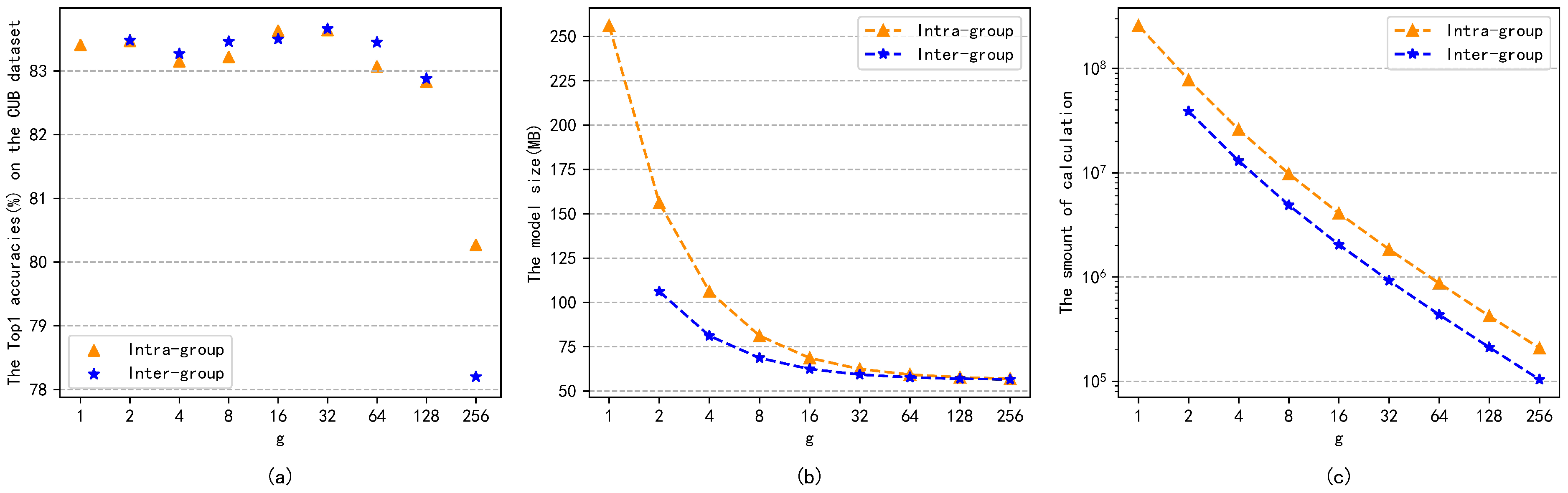
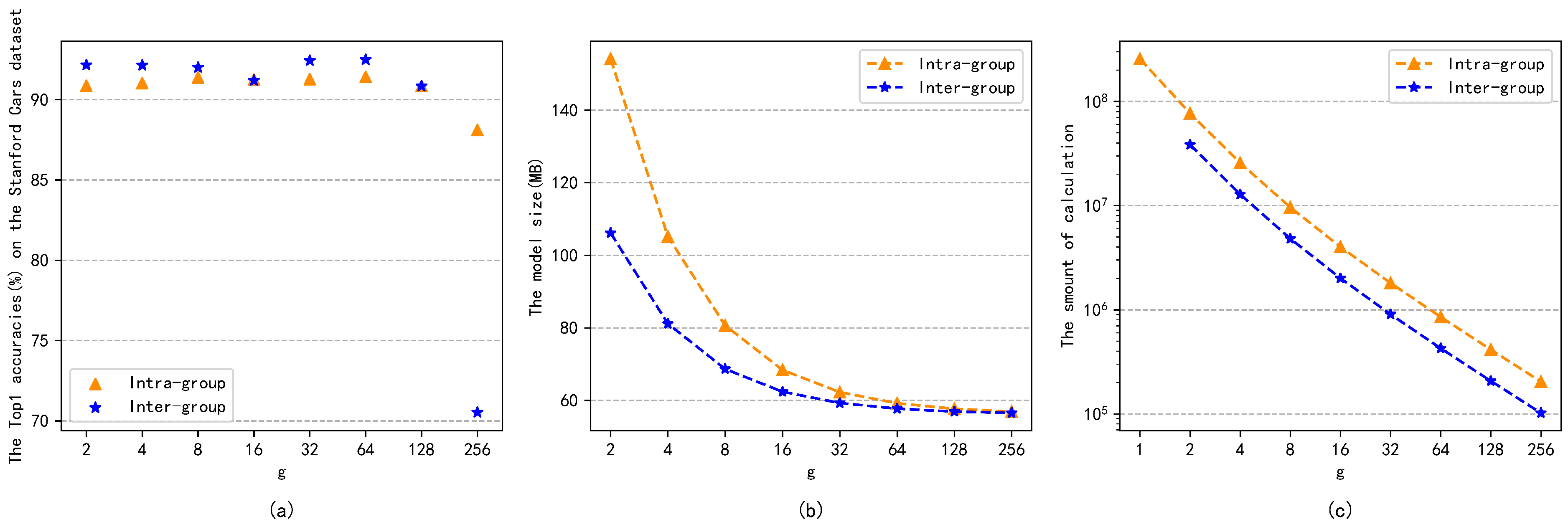
The experiments were carried out on the server of ubuntu system, the code was written by Python and PyTorch [30] deep learning framework. Four NVIDIA GTX 1080 T i GPUs were used for distributed model training and testing. The size of the input image is 448 × 448 and the data augmentation follows the commonly used methods. During the training, the pre-training weight of the model on ImageNet [29] was first loaded and frozen, and the parameters of the full-connection layer between GBP representation and outputs were fine-tuned. During the fine-tuning, the initial learning rate was 0.0003, and the Adam optimizer [31] was adopted to dynamically adjust the learning rate with factor = 0.15, patience = 2, cooldown = 4. After fine-tuning, all frozen parameters were unfreezing, then the learning rate was adjusted to 0.0001. The loss function is multi-classification cross entropy loss function. In all experiments, the same experimental configurations were followed.

4.2. Evaluation

First, convolutional feature extraction network of VGG-16 [27] is used as the backbone network to perform Intra-GBP and Inter-GBP on CUB [1] dataset and Stanford Cars [2] dataset respectively. Then, after grouping bilinear pooling, the obtained representation was used to classify directly by the full-connection layer. The high-order feature layer X extracted from VGG-16 has 512 feature channels, which was divided into g groups, g [ 1 , 2 , 4 , 8 , 16 , 32 , 64 , 128 , 256 ] ; noting that the Intra-GBP degenerates to FBP [15] at g = 1 , and the minimum of g is 2 in Inter-GBP.
The original FBP achieved an accuracy of 84.01% on the CUB dataset, and our reimplementation achieved an accuracy of 83.43%. The experiment results of Intra-GBP and Inter-GBP on the CUB dataset are shown in Figure 3 and Figure 4. With the increasing of g , the accuracy of intra-GBP and Inter-GBP generally increases first and then decreases, the size of the model and the amount of calculation for pooling and classification show a decreasing trend. Intra-GBP achieved the best accuracy of 83.64% at g = 32 on CUB and the best accuracy of 91.42% on Stanford Cars; Inter-GBP achieved the best accuracy of 83.66% at g = 64 on CUB and the best accuracy of 92.49% on Stanford Cars.
In general, both Intra-GBP and Inter-GBP can effectively reduce the dimension of full bilinear representation, and the model based on the two methods can reduce the size of the model and the amount of calculation without causing a loss of model performance within a certain number of g . As discussed, comparing with the Intra-GBP which has inherent redundancy, Inter-GBP can obtain feature representation with less redundancy. In experiments with different backbone networks and datasets, Inter-GBP always performs better. Therefore, in the subsequent experiments, we mainly show the performance of Inter-GBP unless specifically stated.
In order to further verify the performance and effectiveness of GBP with different backbones, we used ResNet-50, ResNet-101 and ResNet-152 as the backbone to perform GBP respectively. With a more powerful backbone, GBP performs better. Table 2 shows the performances of Inter-GBP based on ResNet-50 on CUB and Stanford Cars.
Due to the number of high-order features, the layer is 2048(C = 2048); when using ResNet-50, the range of g goes up, g [ 2 , 4 , 8 , 16 , 32 , 64 , 128 , 256 , 512 , 1024 ] . As can be seen from Table 2, the accuracy of Inter-GBP keeps improving as the number of g keeps increasing. When g = 1024, the accuracy of Inter-GBP on CUB and Stanford Cars reaches the highest accuracy of 85.54% and 92.86% respectively, which are 1.5 and 0.4 percentage points higher than Inter-GBP based on VGG-16. When g goes from 2 to 1024, the model size of Inter-GBP goes from 987.81 MB and 971.81 MB to 99.37 MB and 99.34 MB on CUB and Stanford Cars, respectively.
Noting that the accuracies reach the highest at g = 1024 (maximum number of grouping). It is because feature information extracted from a deep network is more stable compared with a shallow network, and the Inter-GBP representation is sufficiently robust when the maximum number of grouping is used. In all experiments with ResNet as the backbone, more groupings often represent a better performance.

4.3. Comparing with Other Compact Bilinear Pooling

In this section, GBP is compared with other compact bilinear pooling methods [15,17,19,32] in detail. Assuming that the categories to be classified are N, and bilinear pooling is carried out on the feature layers with the size of c × h × w , where c is the feature channels, the height and width of feature layers are h and w (VGG-16: h = w = 28, c = 512; ResNet-50: h = w = 14, c = 2048). For a more intuitive comparison, taking the experiment on CUB as an example, the input size of the images is 448 × 448 . The configurations of the comparative experiment are as follows: g = 128 (VGG-16), g = 1024 (ResNet-50), m = 100, r = 8, d = 8192, N = 200.
The detailed comparisons of different compact bilinear pooling methods are shown in Table 3. The comparison contents include the dimensions of representation, computational complexity of pooling and classifying, and the number of parameters. Under the same configurations, the classification accuracy of different compact bilinear pooling methods based on VGG-16 is shown in Table 4.
As can be seen from Table 3, among all bilinear pooling methods, GBP has the lowest representation dimension. When VGG-16 is used as a backbone, the representation dimension of Inter-GBP is only 0.4% of FBP, the pooling computation is reduced by four orders of magnitude, and the parameters needed to learn are reduced by 99.6%. When ResNet-50 is used as a backbone, the representation dimension of FBP will up to 4.19 million and the parameters needed to learn will reach 3200 MB, while Inter-GBP are 2048 and 1.6 MB respectively. It can be seen intuitively that GBP has a huge advantage in the compression of representation.
Table 4 shows that the performance of GBP is not weaker than or even better than other compact bilinear pooling methods when using the same backbone. The Inter-GBP based on VGG-16 reaches the best accuracy of 92.49% on the Stanford Cars dataset. As an earlier compact bilinear pooling method [17], CBP improves bilinear pooling to some extent and inspires a series of subsequent approaches. iFBP [32] proposes the matrix square-root normalization to improve the performance of the bilinear model, and achieves the best performance on the CUB dataset, but it still requires a lot of computing and storage space. LRBP [19] obtains statistics without performing bilinear pooling, instead using the Frobenius norm as the classification score, which reduces the computation to a certain extent and has advantages in reducing parameters, but it requires the learning of additional projection parameters. Compared with [19], although the performance of GBP based on VGG-16 on the CUB dataset is lower, the pooling computation of GBP is reduced by two orders of magnitude, and the dimension of feature representation obtained by GBP is lower.

4.4. Comparison with the State-of-the-Art
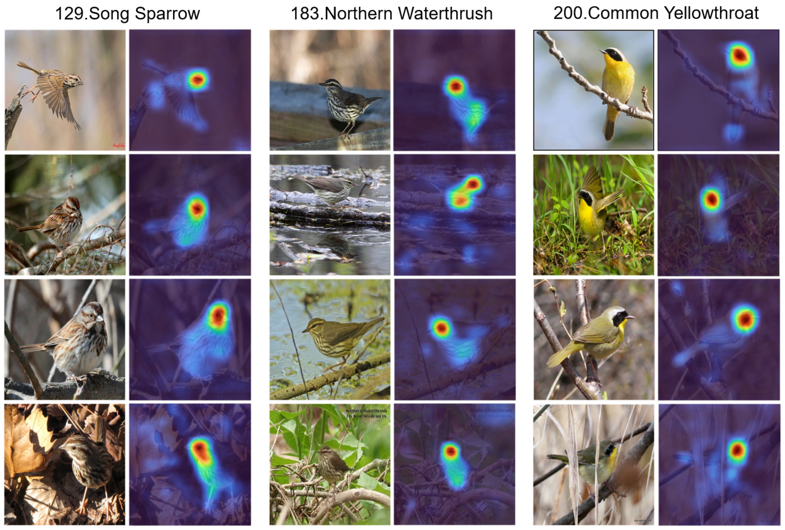
Generally, it is hard to balance accuracy and the complexity of the model when bilinear pooling is applied. With the extreme compression, GBP is able to use more powerful backbones to improve performance. We embedded GBP in different backbones and compared it with other methods. The performances of baselines, full bilinear pooling based methods, compact bilinear pooling based methods, GBP (ours) methods and other state-of-the-art methods relating to channels are shown in Table 5.
Compared with VGG-16, ResNet-50, ResNet-101 and ResNet-152, Inter-GBP improved the accuracy of the CUB dataset by 9, 3.4, 3.5 and 3.6 percentage points respectively after being applied to these backbone networks, and also improved the accuracy of the Stanford Cars dataset by 7.4, 0.7, 1.2 and 1.6 percentage points, respectively. Comparing with the methods based on bilinear pooling and compact bilinear pooling, GBP is the most compact method and achieves the best performance. Especially on the Stanford Cars dataset, Inter-GBP improves the best performance of compact bilinear pooling from 91.80% to 94.22%.
In addition, due to lack of simplicity and convenience, few papers apply compact bilinear pooling approaches to high-performing backbones. We also tried to perform other compact BP on better backbones, but the result is not good enough. GBP compresses the bilinear representation to the extreme so that it can be used with more powerful backbones to achieve competitive performance.
The grouping operation of GBP is performed at the channel level. Compared with other state-of-the-art methods relating to channels [16,36,37,38,39], GBP shows a performance as good as or even better than these methods.
The spatially weighted pooling (SWP) [36] strategy was proposed to improve the robustness and effectiveness of the feature representation, compared with SWP, GBP can improve the performance of the model better when combined with different backbones. Ref. [37] devised a novel model Hierarchical Bilinear Pooling with Aggregated Slack Mask (HBPASM) to generate a RoI-aware image feature representation for better performance, ref. [16] first proposed to obtain a better feature representation by adjusting channel dimensions and performing the Hadamard product between different hierarchical feature layers, but this approach only performs well when using VGG as the backbone, the generalization performance is poor. Mutual-channel loss [39] achieved the state-of-the-art performance when implemented on top of common base networks. Channel permutation and weighted combination regularization in [38] also showed its effectiveness. These methods achieved the state-of-the-art in different ways. Compared with these methods, GBP is simple and easy to implement and has good generalization ability; the Inter-GBP achieves 94.22% accuracy on the Stanford Cars dataset, which is the best accuracy.
In general, GBP not only achieves the best experimental results among methods based on bilinear pooling, but also shows a competitive performance and greater potential compared with other fine-grained image classification methods.

4.5. Visualization

To visually demonstrate the recognition of fine-grained images by the GBP based model, as shown in Figure 5, we visualized the model’s response to the input images of CUB dataset. We compute the magnitude of feature activations averaged across feature channels as the attention of the model and superimpose it to the input image.
Figure 5 shows the model’s visual recognition of images by taking three randomly selected subclasses of birds as examples. It is shown that the model tends to ignore features in the cluttered background and focus on the most discriminative parts of the birds. For example, when recognizing the Northern Waterthrush, similar features such as color and texture exist in the background, but the model focuses primarily on the bird and the distinguishing part of the bird.

5. Conclusions

In order to get compact bilinear representation, we propose grouping bilinear pooling (GBP) for fine-grained image classification in this paper. By dividing the feature layers into different groups and carries out intra-group bilinear pooling or inter-group bilinear pooling, GBP can obtain extreme compact representation. Compared with other compact bilinear methods, GBP achieves the-state-of-the-art. Besides, few papers use a more powerful backbone to achieve bilinear pooling because it is hard to balance accuracy and the complexity of model, but the experiments show that GBP can be embedded into different models as a plug-and-play module and perform well.
With the development of computer vision, a series of peaks that bilinear pooling never reached were achieved by the new methods. As an improvement of bilinear pooling, GBP achieves a competitive performance compared with other approaches. It is worth noting that GBP does not conflict with other fine-grained image classification methods, which means GBP has much more potential. In the future work, we plan to further explore GBP by combining it with other methods in different tasks.

Author Contributions

Conceptualization, R.Z. and J.H.; methodology, R.Z. and J.H.; software, R.Z.; validation, R.Z.; formal analysis, R.Z. and J.H.; investigation, R.Z. and J.H.; resources, J.H.; data curation, J.H. and R.Z.; writing—original draft preparation, R.Z.; writing—review and editing, R.Z. and J.H.; visualization, R.Z. and J.H.; supervision, J.H.; project administration, J.H. All authors have read and agreed to the published version of the manuscript.

Funding

This research received no external funding.

Institutional Review Board Statement

Not applicable.

Informed Consent Statement

Not applicable.

Data Availability Statement

The CUB dataset used in this paper are openly available in [1] and can be found at http://www.vision.caltech.edu/datasets/cub_200_2011/ (accessed on 15 May 2022), and Stanford Cars and are openly available in [2] and can be found at https://ai.stanford.edu/~jkrause/cars/car_dataset.html (accessed on 15 May 2022).

Conflicts of Interest

The authors declare no conflict of interest.

References

  1. Wah, C.; Branson, S.; Welinder, P.; Perona, P.; Belongie, S. The Caltech-UCSD Birds-200-2011 Dataset; Computation & Neural Systems Technical Report, 2010-001; California Institute of Technology: Pasadena, CA, USA, 2011. [Google Scholar]
  2. Krause, J.; Stark, M.; Deng, J.; Fei-Fei, L. 3D Object Representations for Fine-Grained Categorization. In Proceedings of the 2013 IEEE International Conference on Computer Vision Workshops, Sydney, Australia, 2–8 December 2013; pp. 554–561. [Google Scholar] [CrossRef]
  3. Sohaib, M.; Kim, J.M. Data Driven Leakage Detection and Classification of a Boiler Tube. Appl. Sci. 2019, 9, 2450. [Google Scholar] [CrossRef] [Green Version]
  4. Wang, E.; Jiang, Y.; Li, Y.; Yang, J.; Zhang, Q. MFCSNet: Multi-Scale Deep Features Fusion and Cost-Sensitive Loss Function Based Segmentation Network for Remote Sensing Images. Appl. Sci. 2019, 9, 4043. [Google Scholar] [CrossRef] [Green Version]
  5. Chen, L.C.; Papandreou, G.; Kokkinos, I.; Murphy, K.; Yuille, A.L. DeepLab: Semantic Image Segmentation with Deep Convolutional Nets, Atrous Convolution, and Fully Connected CRFs. IEEE Trans. Pattern Anal. Mach. Intell. 2018, 40, 834–848. [Google Scholar] [CrossRef] [PubMed] [Green Version]
  6. Zeiler, M.; Fergus, R. Stochastic Pooling for Regularization of Deep Convolutional Neural Networks. In Proceedings of the International Conference on Learning Representations (ICLR), Scottsdale, AZ, USA, 2–4 May 2013. [Google Scholar]
  7. Yu, D.; Wang, H.; Chen, P.; Wei, Z. Mixed Pooling for Convolutional Neural Networks. In International Conference On Rough Sets and Knowledge Technology; Springer: Cham, Switzerland, 2014; pp. 364–375. [Google Scholar]
  8. Hu, J.; Shen, L.; Albanie, S.; Sun, G.; Wu, E. Squeeze-and-Excitation Networks. IEEE Trans. Pattern Anal. Mach. Intell. 2020, 42, 2011–2023. [Google Scholar] [CrossRef] [PubMed] [Green Version]
  9. Sun, M.; Yuan, Y.; Zhou, F.; Ding, E. Multi-Attention Multi-Class Constraint for Fine-grained Image Recognition. In Proceedings of the European Conference on Computer Vision (ECCV), Munich, Germany, 8–14 September 2018. [Google Scholar]
  10. Lin, T.Y.; Dollár, P.; Girshick, R.; He, K.; Hariharan, B.; Belongie, S. Feature Pyramid Networks for Object Detection. In Proceedings of the IEEE Conference on Computer Vision and Pattern Recognition (CVPR), Honolulu, HI, USA, 21–26 July 2017; pp. 936–944. [Google Scholar] [CrossRef] [Green Version]
  11. Daniilidis, K.; Maragos, P.; Paragios, N. Improving the Fisher Kernel for Large-Scale Image Classification. In European Conference on Computer Vision; Springer: Berlin/Heidelberg, Germany, 2010. [Google Scholar]
  12. Perronnin, F.; Dance, C. Fisher Kernels on Visual Vocabularies for Image Categorization. In Proceedings of the 2007 IEEE Conference on Computer Vision and Pattern Recognition, Minneapolis, MN, USA, 18–23 June 2007; pp. 1–8. [Google Scholar] [CrossRef]
  13. Jégou, H.; Douze, M.; Schmid, C.; Pérez, P. Aggregating local descriptors into a compact image representation. In Proceedings of the 2010 IEEE Computer Society Conference on Computer Vision and Pattern Recognition, San Francisco, CA, USA, 13–18 June 2010; pp. 3304–3311. [Google Scholar] [CrossRef] [Green Version]
  14. Lazebnik, S.; Schmid, C.; Ponce, J. Beyond Bags of Features: Spatial Pyramid Matching for Recognizing Natural Scene Categories. In Proceedings of the 2006 IEEE Computer Society Conference on Computer Vision and Pattern Recognition (CVPR’06), New York, NY, USA, 17–22 June 2006; Volume 2, pp. 2169–2178. [Google Scholar] [CrossRef] [Green Version]
  15. Lin, T.Y.; RoyChowdhury, A.; Maji, S. Bilinear CNN Models for Fine-Grained Visual Recognition. In Proceedings of the 2015 IEEE International Conference on Computer Vision (ICCV), Santiago, Chile, 7–13 December 2015; pp. 1449–1457. [Google Scholar] [CrossRef]
  16. Yu, C.; Zhao, X.; Zheng, Q.; Zhang, P.; You, X. Hierarchical Bilinear Pooling for Fine-Grained Visual Recognition. In Proceedings of the Computer Vision–ECCV 2018, Munich, Germany, 8–14 September 2018; pp. 595–610. [Google Scholar]
  17. Gao, Y.; Beijbom, O.; Zhang, N.; Darrell, T. Compact Bilinear Pooling. In Proceedings of the 2016 IEEE Conference on Computer Vision and Pattern Recognition (CVPR), Las Vegas, NV, USA, 27–30 June 2016; pp. 317–326. [Google Scholar] [CrossRef] [Green Version]
  18. Ni, Z.L.; Bian, G.B.; Wang, G.; Zhou, X.H.; Hou, Z.G.; Xie, X.L.; Chen, H.B.; Li, Z. Pyramid Attention Aggregation Network for Semantic Segmentation of Surgical Instruments. In Proceedings of the AAAI Conference on Artificial Intelligence, New York, NY, USA, 7–12 February 2020; Volume 34. [Google Scholar] [CrossRef]
  19. Kong, S.; Fowlkes, C. Low-Rank Bilinear Pooling for Fine-Grained Classification. In Proceedings of the 2017 IEEE Conference on Computer Vision and Pattern Recognition (CVPR), Honolulu, HI, USA, 21–26 July 2017; pp. 7025–7034. [Google Scholar] [CrossRef] [Green Version]
  20. Zheng, H.; Fu, J.; Zha, Z.J.; Luo, J. Learning Deep Bilinear Transformation for Fine-grained Image Representation. In Advances in Neural Information Processing Systems; Curran Associates, Inc.: Red Hook, NY, USA, 2019; Volume 32. [Google Scholar]
  21. Kar, P.; Karnick, H. Random feature maps for dot product kernels. J. Mach. Learn. Res. 2012, 22, 583–591. [Google Scholar]
  22. Pham, N.; Pagh, R. Fast and scalable polynomial kernels via explicit feature maps. In Proceedings of the 19th ACM SIGKDD International Conference on Knowledge Discovery and Data Mining, Chicago, IL, USA, 11–14 August 2013; pp. 239–247. [Google Scholar] [CrossRef] [Green Version]
  23. Fukui, A.; Park, D.; Yang, D.; Rohrbach, A.; Darrell, T.; Rohrbach, M. Multimodal Compact Bilinear Pooling for Visual Question Answering and Visual Grounding. arXiv 2016, arXiv:1606.01847. [Google Scholar]
  24. Suh, Y.; Wang, J.; Tang, S.; Mei, T.; Lee, K.M. Part-aligned bilinear representations for person re-identification. In Proceedings of the European Conference on Computer Vision (ECCV), Munich, Germany, 8–14 September 2018; pp. 402–419. [Google Scholar]
  25. Yu, T.; Meng, J.; Yuan, J. Multi-view harmonized bilinear network for 3d object recognition. In Proceedings of the IEEE Conference on Computer Vision and Pattern Recognition, Salt Lake City, UT, USA, 18–23 June 2018; pp. 186–194. [Google Scholar]
  26. Hu, J.F.; Zheng, W.S.; Pan, J.; Lai, J.; Zhang, J. Deep bilinear learning for rgb-d action recognition. In Proceedings of the European Conference on Computer Vision (ECCV), Munich, Germany, 8–14 September 2018; pp. 335–351. [Google Scholar]
  27. Simonyan, K.; Zisserman, A. Very Deep Convolutional Networks for Large-Scale Image Recognition. arXiv 2014, arXiv:1409.1556. [Google Scholar]
  28. He, K.; Zhang, X.; Ren, S.; Sun, J. Deep Residual Learning for Image Recognition. In Proceedings of the 2016 IEEE Conference on Computer Vision and Pattern Recognition (CVPR), Las Vegas, NV, USA, 27–30 June 2016; pp. 770–778. [Google Scholar] [CrossRef] [Green Version]
  29. Deng, J.; Dong, W.; Socher, R.; Li, L.J.; Li, K.; Fei-Fei, L. ImageNet: A large-scale hierarchical image database. In Proceedings of the 2009 IEEE Conference on Computer Vision and Pattern Recognition, Miami, FL, USA, 20–25 June 2009; pp. 248–255. [Google Scholar] [CrossRef] [Green Version]
  30. Paszke, A.; Gross, S.; Massa, F.; Lerer, A.; Bradbury, J.; Chanan, G.; Killeen, T.; Lin, Z.; Gimelshein, N.; Antiga, L.; et al. PyTorch: An Imperative Style, High-Performance Deep Learning Library. In Advances in Neural Information Processing Systems; Curran Associates, Inc.: Red Hook, NY, USA, 2019; Volume 32. [Google Scholar]
  31. Kingma, D.; Ba, J. Adam: A Method for Stochastic Optimization. In Proceedings of the International Conference on Learning Representations, Banff, AB, Canada, 14–16 April 2014. [Google Scholar]
  32. Lin, T.Y.; Maji, S. Improved Bilinear Pooling with CNNs. arXiv 2017, arXiv:1707.06772. [Google Scholar]
  33. Gou, M.; Xiong, F.; Camps, O.; Sznaier, M. MoNet: Moments Embedding Network. In Proceedings of the 2018 IEEE/CVF Conference on Computer Vision and Pattern Recognition, Salt Lake City, UT, USA, 18–22 June 2018; pp. 3175–3183. [Google Scholar]
  34. Gao, Z.; Wu, Y.; Zhang, X.; Dai, J.; Jia, Y.; Harandi, M. Revisiting Bilinear Pooling: A Coding Perspective. In Proceedings of the AAAI Conference on Artificial Intelligence, New York, NY, USA, 7–12 February 2020; pp. 3954–3961. [Google Scholar]
  35. Liao, Q.; Wang, D.; Holewa, H.; Xu, M. Squeezed Bilinear Pooling for Fine-Grained Visual Categorization. In Proceedings of the 2019 IEEE/CVF International Conference on Computer Vision Workshop (ICCVW), Seoul, Korea, 27–28 October 2019; pp. 728–732. [Google Scholar] [CrossRef]
  36. Hu, Q.; Wang, H.; Li, T.; Shen, C. Deep CNNs with Spatially Weighted Pooling for Fine-Grained Car Recognition. IEEE Trans. Intell. Transp. Syst. 2017, 18, 3147–3156. [Google Scholar] [CrossRef]
  37. Tan, M.; Wang, G.; Zhou, J.; Peng, Z.; Zheng, M. Fine-Grained Classification via Hierarchical Bilinear Pooling with Aggregated Slack Mask. IEEE Access 2019, 7, 117944–117953. [Google Scholar] [CrossRef]
  38. Luo, W.; Zhang, H.; Li, J.; Wei, X.S. Learning Semantically Enhanced Feature for Fine-Grained Image Classification. IEEE Signal Process. Lett. 2020, 27, 1545–1549. [Google Scholar] [CrossRef]
  39. Chang, D.; Ding, Y.; Xie, J.; Bhunia, A.K.; Li, X.; Ma, Z.; Wu, M.; Guo, J.; Song, Y.Z. The Devil is in the Channels: Mutual-Channel Loss for Fine-Grained Image Classification. IEEE Trans. Image Process. 2020, 29, 4683–4695. [Google Scholar] [CrossRef] [PubMed] [Green Version]
Figure 1. The architecture of Bilinear CNN. X is the high-order features extracted by CNN. Z is the full bilinear representation obtained by bilinear pooling.
Applsci 12 05063 g001
Figure 2. (a) Full bilinear pooling (FBP), bilinear pooling is performed in pairs in all feature layers. (b) Compact bilinear pooling (CBP), the feature layer is mapped and the Hadamard product is used to simplify bilinear pooling. (c) Low-rank bilinear pooling (LRBP), which obtains statistics without performing bilinear pooling, instead using the Frobenius norm as the classification score. (d) The intra-group bilinear pooling (Intra-GBP), bilinear pooling performs in each grouped feature layer group. (e) The inter-group bilinear pooling (Inter-GBP), bilinear pooling performs between two different grouped feature layer groups.
Applsci 12 05063 g002
Figure 3. (a) The classification accuracy of Intra-GBP and Inter-GBP based on VGG-16 on CUB dataset; (b) The corresponding model size with different g (including backbone CNN); (c) The amount of calculation for pooling and classification.
Applsci 12 05063 g003
Figure 4. (a) The classification accuracy of Intra-GBP and Inter-GBP based on VGG-16 on Stanford Cars dataset; (b) The corresponding model size with different g (including backbone CNN); (c) The amount of calculation for pooling and classification.
Applsci 12 05063 g004
Figure 5. The recognition of fine-grained images by the GBP based model. The brighter the region is, the more attention the model pays to it.
Applsci 12 05063 g005
Table 1. Dataset Details.
DatasetTrainingTestingCategory
CUB [1]59945794200
Stanford Cars [2]81448041196
Table 2. The performances of Inter-GBP based on ResNet-50 on CUB dataset and Stanford Cars dataset.
The Groups2481632641282565121024
CUB (%)83.7984.1985.1385.2885.2385.1185.0785.2185.3285.54
Model size (MB)987.81497.81297.81197.81147.81122.81110.31104.06100.9499.37
Stanford Cars (%)92.1192.3492.3592.2992.3392.4992.6192.7592.7492.86
Model size (MB)971.81489.81293.81195.81146.81122.31110.06103.94100.8799.34
Table 3. Comparison of different compact bilinear pooling methods. We used VGG-16 and ResNet-50 as the backbone respectively to compare the computational complexity, representation dimensions and the parameters needed to be learned (excluding the backbone network).
BackboneMethodDimensionComputingParameters
PoolingClassifyingTotalProjectionClassifierTotal
VGG-16FBP [15] c 2 [262 K] O ( h w c 2 ) O ( N c 2 ) 257,949,6960 N c 2 200 MB
iFBP [32] c 2 [262 K] O ( h w c 2 ) O ( N c 2 ) 257,949,6960 N c 2 200 MB
CBP-TS [17]d [10 K] O ( h w ( c + d l o g d ) ) O ( N d ) 85,532,672 2 c N d 8 MB
CBP-RM [17]d [10 K] O ( h w c d ) O ( N d ) 3,289,972,736 2 c d N d 48 MB
LRBP-I [19] m h w [78 K] O ( h w c m ) O ( N r m h w ) 165,580,800 c m N r m 0.8 MB
LRBP-II [19] m 2 [10 K] O ( h w ( c m + m 2 ) ) O ( N r m 2 ) 63,980,800 c m N r m 0.8 MB
Intra-GBP (ours) c 2 / g [2 K] O ( h w c 2 / g 2 ) O ( N c 2 / g ) 422,1440 N c 2 / g 1.6 MB
Inter-GBP ( o u r s ) c 2 / 2 g [1 K] O ( h w c 2 / 2 g 2 ) O ( N c 2 / 2 g ) 211,0720 N c 2 / 2 g 0.8 MB
ResNet-50FBP [15] c 2 [4194 K] O ( h w c 2 ) O ( N c 2 ) 1,660,944,3840 N c 2 3200 MB
Intra-GBP ( o u r s ) c 2 / g [4 K] O ( h w c 2 / g 2 ) O ( N c 2 / g ) 819,9840 N c 2 / g 3.2 MB
Inter-GBP ( o u r s ) c 2 / 2 g [2 K] O ( h w c 2 / 2 g 2 ) O ( N c 2 / 2 g ) 409,9920 N c 2 / 2 g 1.6 MB
Table 4. The performances of different compact bilinear pooling methods on CUB dataset and Stanford Cars dataset. (Based on VGG-16).
MethodFBP [15]iFBP [32]CBP-TS [17]CBP-RM [17]LRBP [19]Intra-GBPInter-GBP
CUB (%)84.0185.8084.0083.8684.2183.6483.66
Cars (%)91.1892.1090.1989.5490.9291.4292.49
Table 5. The performances of different methods on CUB dataset and Stanford Cars dataset. From top to bottom, the five blocks respectively list the baselines, full bilinear pooling based methods, compact bilinear pooling based methods, other state-of-the-art methods relating to channels and our method.
MethodBackboneDimensionParametersCUB (%)Stanford Cars (%)
VGG-16 [27]-25 K20 MB74.5985.05
ResNet-50 [28]-2 K1.6 MB82.1592.19
ResNet-101 [28]-2 K1.6 MB82.5892.56
ResNet-152 [28]-2 K1.6 MB82.7492.64
FBP [15]VGG-16260 K200 MB84.0191.18
iFBP [32]85.8092.10
MoNet-FBP [33]86.4091.80
CBP [17]VGG-1610 K8 MB84.0090.19
LRBP [19]10 K0.8 MB84.2190.90
MoNet-TS [33]10 K8 MB85.7090.80
FBC [34]8 K6.4 MB84.30-
SBP-EN [35]10 K8 MB84.5090.90
SWP [36]VGG-16---90.70
ResNet-50---92.30
ResNet-101---93.10
HBPASM [37]ResNet-34--86.8092.80
HBP [16]VGG-1624 K19 MB87.0193.70
SEF [38]VGG-16--81.1088.30
ResNet-50--87.3094.00
MC-loss [39]ResNet-50--87.3093.70
Inter-GBPVGG-161 K0.8 MB83.6692.49
ResNet-502 K1.6 MB85.5492.86
ResNet-1012 K1.6 MB86.1093.76
ResNet-1522K1.6 MB86.3194.22
Publisher’s Note: MDPI stays neutral with regard to jurisdictional claims in published maps and institutional affiliations.

