Railway Bridge Condition Monitoring Using Numerically Calculated Responses from Batches of Trains

Abstract

This study introduces a novel method to determine apparent profile of the track and detect railway bridge condition using sensors on in-service trains. The concept uses a type of Inverse Newmark-β integration scheme on data from a batch of trains. In a self-calibration process, an optimization algorithm is used to find vehicle dynamic properties and speed. For bridge health monitoring, the apparent profile of the bridge is first determined, i.e., the true profile plus components of ballast and bridge deflection under the moving train. The apparent profile is used, in turn, to calculate the moving reference deflection influence line, i.e., the deflection due to a moving (static) unit load. The moving reference influence line is shown to be a good indicator of bridge stiffness. This numerical approach is assessed using an elaborate finite element model operated by an independent research group. The results show that the moving reference influence line can be found accurately and that it constitutes an effective indicator of the condition of a bridge.

1. Introduction

Traditional monitoring of railway infrastructure often involves on-track visual inspections. This approach is not entirely satisfactory due to issues of cost, safety, and speed of implementation. For structures such as bridges, direct monitoring has become popular in the literature [1,2,3,4,5]. This measures the response directly using sensors installed in the structure. It needs several sensors to be mounted, which generally cannot be reused in other structures.

Vehicle-based techniques (drive-by) have long been used to detect the geometrical properties of track, such as the profile and rail condition [6,7]. Specialist Track Recording Vehicles (TRVs) are used for this purpose in accordance with European Standard EN 13848 [8] but are expensive and may disrupt scheduled services. Using in-service vehicles to provide data for railway infrastructure maintenance managers has the potential to complement or replace TRV data and has the advantage of providing real-time information at a significantly reduced cost. Cantero and Basu [9] propose a wavelet-based assessment methodology to detect local track irregularities using accelerations measured in moving vehicles. A wavelet-based indicator is proposed to facilitate the recognition of deteriorated segments. OBrien et al. [10] develop a method to determine the longitudinal profile using bogie vertical accelerations and angular velocities resulting from train/track dynamic interaction. The railway track profile elevations, determined by Cross Entropy (CE) optimisation, are those that generate a vehicle response which best fits the measurements in a railway carriage bogie. Yang et al. [11] develop an effective technique to identify the track modulus, i.e., the foundation stiffness of the rails, using the contact-point response of a moving test vehicle. It is shown that the track modulus can be successfully identified via the first rail frequency extracted from the contact-point response. Tsunashima et al. [12] propose a portable condition monitoring system for track which is easily integrated into in-service vehicles. It can estimate rail irregularities from the vertical and lateral accelerations of the car body. Kobayashi et al. [13] estimate track irregularity from car-body motions using a Kalman Filter. Ren et al. [14] introduce a new two-stage direct integration approach to find the track profile much more efficiently than the CE optimisation method. The railway car model is represented using the half-car model twice. The calculated track profile is similar to a ‘true’ profile and can be used to monitor the condition of the track.

The drive-by method is examined by a field test in some research. The numerical method developed in OBrien et al. [10] was subsequently tested in the field by OBrien et al. [15]. A good match is achieved between the inferred longitudinal profiles and the surveyed track profile. Real et al. [16] develop a new method to determine railway vertical profile using accelerations recorded on the bogies of in-service trains. It is validated by a field test on Line 9 of the Madrid underground. Wei et al. [17] use the bogie and the car body acceleration sensors to estimate track irregularities. The acceleration signals are pre-processed with filters. Subsequently, the track alignments are obtained by double integration of the signals. Field tests were carried out on the Shanghai metro Line 1 to demonstrate the effectiveness of the proposed track inspection system. Paixao et al. [18] use a smartphone to obtain constant acceleration measurements on in-service trains to assess structural performance and geometrical degradation of the tracks. Cross-correlation values were obtained between the standard deviations of the longitudinal level and the measured vertical accelerations and are proposed as a means to identify critical situations that affect the performance of the track.

The drive-by method of bridge health monitoring has advantages compared with the conventional direct monitoring approach. It is mobile, economic, and efficient [19]. Malekjafarian et al. [20] review drive-by, also known as indirect, methods of monitoring highway bridges. Most methods are based on the identification of dynamic characteristics of the bridge from responses measured in the vehicle, such as natural frequencies, mode shapes, and damping [21,22,23,24,25]. Some methods detect bridge damage directly from the interaction between the vehicle and bridge without using the conventional structural dynamic properties. OBrien and Keenahan [26] use CE optimisation to determine the Apparent Profile (AP), where the displacements recorded by the sensors are used as the inputs. The time-shifted difference in the AP is proposed to detect bridge damage and numerical results show that it has good potential as a damage indicator. Elhattab et al. [27] calculate APs from on-board sensors and then subtract them to calculate the ‘bridge displacement profile difference’ (BDPD), which is proposed as another bridge damage indicator. Keenahan and OBrien [28] used a Traffic Speed Deflectometer (TSD) to detect damage in bridges. The data gathered from the TSD are post-processed and time-shifted curvature, without pitch; this is used as the damage indicator. The time-shifted curvature is derived from the displacements and is proposed as a novel damage indicator, which removes the influence of the road profile and all vehicle motions except for pitch.

For railway bridges, Quirke et al. [29] detect damage through comparison of APs sensed by the passing vehicle. The APs are calculated using the CE optimisation method that generates a vehicle dynamic response most similar to the measured input. APs for a number of damage scenarios are inferred and compared over time to detect damage. Fitzgerald et al. [30] develop a method to detect the presence of railway bridge scour using bogie acceleration measurements from a passing train. A scour indicator is defined as the difference in average Continuous Wavelet Transform coefficients between healthy and scoured batches of train crossings. The result shows that this indicator is quite effective at detecting the presence of scour and its location.

Some field tests of railway bridge monitoring using onboard train measurements are introduced in the following articles. Various tests have been conducted at the Bridge Deflection Test Facility (BDTF) at the Transportation Technology Center, USA. A track deflection measurement system (TDMS) and a track geometry measurement system (TGMS) have been tested on different trains. They investigate the potential for using onboard technology to detect bridge impairment or changes in bridge behaviour [31]. Rakoczy et al. [32] present simulation and field test results of a freight car and locomotive running on a railway bridge. Simulations and tests are used to improve the onboard measurement capability of such a system and the new configuration of accelerometers is shown to provide useful results for bridge condition evaluations. Displacements are derived from the acceleration data. Then, the results from different bridge conditions are compared and relative deflections are calculated to identify the change in bridge condition. Micu et al. [33] introduce a field study of drive-by bridge monitoring using acceleration measurements on an instrumented train. The dynamic responses of the train signals are used to detect the existence and location of a stiffer part of the viaduct where two spans were replaced. The results show that instrumented trains can be successfully used to monitor bridge condition and to identify the need for repair or rehabilitation.

This article presents a novel method of determining AP of the track and detecting bridge damage using batches of trains. In this context, AP is deemed to include the unloaded surface profile and the deflections of the track under the applied train load. Firstly, an Inverse Newmark-β algorithm is introduced to calculate AP from a train measurement. Following this, the concept of using a batch of trains is introduced to find the profile, without prior knowledge of the train masses and velocities. This is effectively a train self-calibration process. Moving reference influence lines are calculated from APs of the bridge which are shown to be a good indication of the bridge behaviour and condition. A blind test is used to validate these methods: bridge damage is calculated for simulated data provided by an independent laboratory, without prior knowledge of the damage levels used in the simulations.

2. Model Description

In this research, the vehicle is simulated crossing the track and bridge in a train–track–bridge (TTB) dynamic system. More detailed information of TTB systems is available in Cantero et al. [34]. This model is used by the Norwegian team to provide simulated measured data for the blind test. It is described briefly in this section.

2.1. Vehicle Model

The train is represented by the two-dimensional (2D) 4-axle railway carriage model shown in Figure 1. The vehicle model includes lumped masses, rigid bars, springs, and dampers. There are 10 degrees of freedom (DOFs) in this vehicle model: vertical translation and rotation about the centre of gravity for the car body and bogies and vertical translation for each wheelset. The wheels are fixed to the track with no separation being permitted. This reduces the system to six DOFs. In this model, each wheel is modelled with a mass ($m_w$). It is connected to the bogie by a primary suspension represented by a spring ($k_p$) and a viscous damper ($c_p$) in parallel. The bogies are represented as rigid bars with mass ($m_b$) and moment of inertia ($I_b$), whereas the main body of the vehicle is also represented as a rigid bar with mass ($m_v$) and moment of inertia ($I_v$). Springs ($k_s$. ) and dampers ($c_s$) represent the secondary suspensions to connect the bogies to the main body. The distances between the car body centre of mass and the bogie pivots are $L_{v1}$ and $L_{v2}$. Similarly, $L_{b1}$, $L_{b2}$,$L_{b3}$, and $L_{b4}$ are the distances between the bogie centres of mass and the wheels. Vehicle models of this type have been used in many studies [35,36].

Assuming small rotations, a linearised system of equations of motion is adopted [37] and can be expressed in matrix form:

$$M_v\ddot{u}+C_v\dot{u}+K_{v}u=F$$

(1)

where $M_v$, $C_v$, and $K_v$ are the mass, damping, and stiffness matrices of the vehicle, respectively. The vectors $\ddot{u}$,$\dot{u,}$ and $u$ represent the vehicle accelerations, velocities, and displacements, respectively and $F$ contains the external forces applied to the vehicle. All matrices and vectors are introduced in the following equations:

$$\ddot{u}=\left\{\begin{array}{c}\begin{array}{c}\begin{array}{c}{\ddot{u}}_v\\ {\ddot{u}}_{b1}\end{array}\\ {\ddot{u}}_{b2}\\ {\ddot{\theta }}_v\end{array}\\ {\ddot{\theta }}_{b1}\\ {\ddot{\theta }}_{b2}\end{array}\right\}$$

(2)

$$\dot{u}=\left\{\begin{array}{c}\begin{array}{c}\begin{array}{c}{\dot{u}}_v\\ {\dot{u}}_{b1}\end{array}\\ {\dot{u}}_{b2}\\ {\dot{\theta }}_v\end{array}\\ {\dot{\theta }}_{b1}\\ {\dot{\theta }}_{b2}\end{array}\right\}$$

(3)

$$u=\left\{\begin{array}{c}\begin{array}{c}\begin{array}{c}{u}_v\\ u_{b1}\end{array}\\ u_{b2}\\ {\theta }_v\end{array}\\ {\theta }_{b1}\\ {\theta }_{b2}\end{array}\right\}$$

(4)

$$F=\left\{\begin{array}{c}\begin{array}{c}{m}_{v}g\\ m_{b1}g+k_{p1}{r}_{w1}+c_{p1}{r}_{w1}^{\prime }+k_{p2}{r}_{w2}+c_{p2}{r}_{w2}^{\prime }\end{array}\\ m_{b2}g+k_{p3}{r}_{w3}+c_{p3}{r}_{w3}^{\prime }+k_{p4}{r}_{w4}+c_{p4}{r}_{w4}^{\prime }\\ 0\\ L_{b11}\left(k_{p1}{r}_{w1}+c_{p1}{r}_{w1}^{\prime }\right)-L_{b12}\left(k_{p2}{r}_{w2}+c_{p2}{r}_{w2}^{\prime }\right)\\ L_{b21}\left(k_{p3}{r}_{w3}+c_{p3}{r}_{w3}^{\prime }\right)-L_{b22}\left(k_{p4}{r}_{w4}+c_{p4}{r}_{w4}^{\prime }\right)\end{array}\right\}$$

(5)

$$M_v=diag\left[\begin{array}{cccccc}{m}_v& m_{b1}& m_{b2}& J_v& J_{b1}& J_{b2}\end{array}\right]$$

(6)

$$K_v=\left[\begin{array}{cccccc}{k}_{s1}+k_{s2}& -k_{s1}& -k_{s2}& L_{v1}{k}_{s1}-L_{v2}{k}_{s2}& 0& 0\\ -k_{s1}& k_{p1}+k_{p2}+k_{s1}& 0& -L_{v1}{k}_{s1}& L_{b11}{k}_{p1}-L_{b12}{k}_{p2}& 0\\ -k_{s2}& 0& k_{p3}+k_{p4}+k_{s2}& L_{v2}{k}_{s2}& 0& L_{b21}{k}_{p3}-L_{b22}{k}_{p4}\\ L_{v1}{k}_{s1}-L_{v2}{k}_{s2}& -L_{v1}{k}_{s1}& L_{v2}{k}_{s2}& L_{v1}{}^2{k}_{s1}+L_{v2}{}^2{k}_{s2}& 0& 0\\ 0& L_{b11}{k}_{p1}-L_{b12}{k}_{p2}& 0& 0& L_{b11}{}^2{k}_{p1}+L_{b12}{}^2{k}_{p2}& 0\\ 0& 0& L_{b21}{k}_{p3}-L_{b22}{k}_{p4}& 0& 0& L_{b21}{}^2{k}_{p3}+L_{b22}{}^2{k}_{p4}\end{array}\right]$$

(7)

$$c_v=\left[\begin{array}{cccccc}{c}_{s1}+c_{s2}& -c_{s1}& -c_{s2}& L_{v1}{c}_{s1}-L_{v2}{c}_{s2}& 0& 0\\ -c_{s1}& c_{p1}+c_{p2}+c_{s1}& 0& -L_{v1}{c}_{s1}& L_{b11}{c}_{p1}-L_{b12}{c}_{p2}& 0\\ -c_{s2}& 0& c_{p3}+c_{p4}+c_{s2}& L_{v2}{c}_{s2}& 0& L_{b21}{c}_{p3}-L_{b22}{c}_{p4}\\ L_{v1}{c}_{s1}-L_{v2}{c}_{s2}& -L_{v1}{c}_{s1}& L_{v2}{c}_{s2}& L_{v1}{}^2{c}_{s1}+L_{v2}{}^2{c}_{s2}& 0& 0\\ 0& L_{b11}{c}_{p1}-L_{b12}{c}_{p2}& 0& 0& L_{b11}{}^2{c}_{p1}+L_{b12}{}^2{c}_{p2}& 0\\ 0& 0& L_{b21}{c}_{p3}-L_{b22}{c}_{p4}& 0& 0& L_{b21}{}^2{c}_{p3}+L_{b22}{}^2{c}_{p4}\end{array}\right]$$

(8)

2.2. Track Model

The track is modelled as a beam supported on spaced sprung mass systems (Figure 2) corresponding to the railway sleepers. The rail is modelled by beam elements in a finite element framework. In this three-layer sprung mass system, the masses represent the sleeper, $m_S$ and ballast, $m_{BA}$. The various layers are connected by spring and damping systems which represent pad, ballast and sub-ballast, with respective properties: $k_P$ and $c_P$; $k_{BA}$ and $c_{BA}$; and $k_{SB}$ and $c_{SB}$. A surface profile is included on the track. Similar models have been used by other researchers [38,39].

2.3. Bridge Model

The bridge/culvert is modelled using a finite element discretization (Figure 3). Behind the walls (abutments), it is filled with soil which is represented by an additional layer of springs with stiffness $k_{soil}$. On top of the beam there is a track which is also modelled as a beam (of much less flexural rigidity). The track beam is supported on a sprung mass system which represents pads, sleepers, and a ballast.

The vehicle and track/bridge model are coupled together via the wheel/rail interaction, i.e., the DOFs of the wheels and the DOFs of the rail are combined. Each of the subsystems can be defined by a set of equations of motion. The coupling of the subsystems is addressed by the coupled equations of motion of the complete model. The equations of motion are solved using the Newmark-β numerical integration scheme.

3. Inverse Newmark-β Method to Calculate AP

As shown in previous work, for a road or a track on infinitely rigid supports, the profile can be determined by CE optimization using bogie vertical accelerations and angular velocities [10]. This approach is shown to be effective but computationally intensive and therefore impractical for kilometres of track data. Keenahan et al. [40] propose a much more efficient Inverse Newmark-β integration process to calculate the AP. The Inverse Newmark-β concept is extended here from Keenahan’s 2-axle 4-degree-of-freedom half car to a 4-axle railway carriage model.

The standard Newmark-β integration scheme is used to calculate the accelerations, velocities, and displacements in a vehicle, {$\ddot{u}$}, {$\dot{u}$}, and {$u$} due to a specified vehicle excitation (e.g., surface profile), i.e., to find {$\ddot{u}$} according to Equation (1).

The inverse Newmark-β concept uses measured accelerations and rates of rotation to find the excitation forces or the surface profile that generates them. In the standard Newmark-β integration scheme, the acceleration, {$\ddot{u}$}, can be calculated from {$u$}:

$${\ddot{u}}_{t+\Delta t}=\left(u_{t+\Delta t}-u_t\right)a_0-a_2{\dot{u}}_t-a_3{\ddot{u}}_t$$

(9)

In the inverse problem, the displacement, {$u$} can be determined from measured acceleration:

$$u_{t+\Delta t}=({\ddot{u}}_{t+\Delta t}+a_2{\dot{u}}_t+a_3{\ddot{u}}_t)/a_0+u_t$$

(10)

where $a_0,a_2$, and $a_3$ are integration constants of the Newmark-β method.

For the 4-axle car model, accelerations and rates of rotation on bogies, ${\ddot{u}}_b$ and ${\dot{\theta }}_b$, are known inputs. Other parameters, ${\dot{u}}_b,u_b,{\ddot{\theta }}_b$, and ${\theta }_b$ of the bogies can be calculated from the known inputs according to the inverse Newmark-β concept. Then, using the equations of motion of the main body, the displacement and rotation of the carriage ($u_v$ and ${\theta }_v$) can be calculated. Accelerations and velocities of the body, ${\ddot{u}}_v,{\dot{u}}_v,{\dot{\theta }}_v,\mathrm{and}{\ddot{\theta }}_v$, can be calculated from $u_v$ and ${\theta }_v$. Therefore, all the terms on the left side of Equation (1) are known and on the right side of Equation (1), $F$, can be found. Finally, the AP that excited the vehicle and caused the accelerations, $r_w$, can be determined by solving Equation (5). Details of this processes are shown in Appendix A.

Here, a 100 m railway track with a profile and a 4-axle railway carriage model vehicle of known properties are used to generate the bogie vertical accelerations and angular velocities. The vehicle properties and speed are shown in

Table 1. Vehicle properties used to calculate the AP.

Property	Symbol	Unit	Value
Carriage body mass	$m_v$	kg	32.4 × 103
Carriage body moment of inertia	$I_v$	kg m2	1.99 × 106
Speed	$v$	m/s	33
Bogie mass	$m_b$	kg	2615
Bogie moment of inertia	$I_b$	kg m2	1476
Wheelset mass	$m_w$	kg	1813
Primary suspension stiffness	$k_p$	N/m	2.4 × 106
Secondary suspension stiffness	$k_s$	N/m	0.86 × 106
Primary suspension damping	$c_p$	N s/m	7 × 103
Secondary suspension damping	$c_s$	N s/m	16 × 103
Distance between bogie centre of gravity and wheelsets	$L_b$	m	1.28
Distance between main body centre of gravity and bogies	$L_v$	m	9.5

. These signals are then taken as inputs and used to back calculate the AP using the Inverse Newmark-β method. The calculated results are compared with the original ‘true’ AP in Figure 4. The true AP is the AP used to generate the bogie vertical accelerations and angular velocities. The calculated result is from the first axle of this train. The calculated AP has similar local features to the ‘true’ AP but is displaced downwards by a ‘drift’ effect that results from an accumulation of numerical inaccuracies. As the drift effect is very low frequency, it has a negligible effect on the train/track dynamic interaction.

4. Monitoring Track Using Self-Calibrating Batches of Vehicles

In the previous section, it is shown that the AP can be calculated from measured vertical accelerations and angular velocities if the properties of the train are known. Trains often make multiple runs on the same route. Hence, an instrumented carriage will provide data from multiple runs for which some ‘global’ vehicle properties, such as spring stiffnesses and damping coefficients, are the same but other ‘local’ properties, such as speed, mass, and moment of inertia are not. In this study, the global properties are assumed to have been determined in a global calibration exercise to some degree of accuracy. A self-calibration process is presented for calculation of the local properties, which are taken to be different for every run of the train.

As first proposed by Keenahan et al. [40] for 2-axle vehicles, batches of runs of the same vehicle will be used to calculate profiles and to determine the local properties. However, in this case, unlike Keenahan et al., the track is supported on springs. Keenahan’s concept is that every vehicle is subjected to the same (rigidly supported) surface profile. Hence, whatever the vehicle properties, processing its measurements should give the same surface profile as all other runs. Keenahan et al. use this phenomenon to self calibrate the system, finding the surface profile and the properties for every vehicle in the batch. CE optimization is used to find those train properties that imply the same profile for all runs in the batch.

In this article, the fleet monitoring concept is extended to 4-axle railway carriages passing over tracks on spring supports. As the surface profile is no longer on rigid supports, the track deflects under the weight of the train. From the vehicle’s perspective, it is excited by an AP made up of the unloaded surface profile and deflection components due to deformation of the track under its own weight. The hypothesis is that the system can be calibrated by forcing all calculated APs to be the same (for all trains).

Like the Genetic Algorithm, CE is a population-based method of optimization which considers multiple feasible solutions in each generation (or iteration) of the process [41]. Firstly, a population of trial values of the vehicle parameter vector is generated. For calibration of a particular batch, global train-specific parameters (such as vehicle stiffnesses) are assumed to be known and only local run-specific parameters are needed. In this case, the local parameter vector has three components: carriage mass ($m_v$), moment of inertia ($I_v$), and speed ($v$).

In the CE process, a population of parameter vectors is randomly generated from a normal distribution using Monte Carlo simulation. Using the generated masses, moments of inertia, speeds, and known global properties, the AP is calculated from the bogie vertical accelerations and angular velocities using the Inverse Newmark-β method. This process is repeated for all vehicles so the total number of unknown local properties in the vector is 3 n_b, where n_b is the number of runs in the batch.

In the first generation of solutions, the n_b generated APs will not be correct as the (run-specific) train properties will not generally be correct. However, better trials of the 3 n_b parameters can be identified as those for which the calculated APs are closest to each other. Thus, an ‘elite set’ of the trials with the best property vectors can be identified using an objective function that captures similar APs within the batch. While more sophisticated measures of ‘similarity’ of APs are possible, a simple approach is adopted here, and the objective function is defined as the sum of squared differences between each AP and the mean of all calculated APs. Hence, the objective function for the $j\mathrm{th}$ trial solution, $O_j$, is the sum of squared differences of the AP generated by this trial vector of 3 n_b properties and the mean AP generated by all vehicles.

$$O_j={\displaystyle \sum }_h{\displaystyle \sum }_{i=1}^{n_b}{\displaystyle \sum }_k{\left(r_{h,i,j,k }-{\overline{r}}_{h,j,k}\right)}^2$$

(11)

where $r_{h,i,j,k}$is the $k\mathrm{th}$ AP elevation in the $j\mathrm{th}$ trial under the $h\mathrm{th}$ axle of the $i\mathrm{th}$ vehicle in the batch and ${\overline{r}}_{h,j,k}$ is mean AP in the $j\mathrm{th}$ trial under the $h\mathrm{th}$ axle of the $n_b$ vehicles of the batch:

$${\overline{r}}_{h,j,k}=\frac{1}{n_b}{\displaystyle \sum }_{i=1}^{n_b}{r}_{h,i,j,k}$$

(12)

As AP elevations are defined in space and these calculations are processed at fixed time intervals arising from the scan rate of the data, there needs to be a conversion to allow for the different speed of each run. For this purpose, the mean speed for all runs is used as the reference and the data for each individual run is interpolated to find the AP elevations corresponding to this reference speed.

In the CE optimization, the elite set is defined as the 10% of trial solutions that have the least values for the objective function. The vector mean and standard deviation of this elite set, μ and σ, are calculated and used as the basis to generate the next generation of trial vehicle properties by Monte Carlo simulation. This process is repeated until convergence. A number of restarts of the process are used to avoid premature convergence [42]. In each restart, the vector mean is retained but the standard deviation is reset to its initial value.

5. Bridge Health Monitoring

When trains are traveling on track only (off-bridge), their data can be used to monitor AP, which is a valuable measure of track condition. In addition, as was shown above, off-bridge data can be used to determine local train dynamic properties. When a train crosses a bridge, it is subject to another AP, this time made up of a combination of the track profile, track deformation, and elements of bridge deflection. Because the AP includes bridge deflections, it contains information about the bridge response to applied load and ultimately about the bridge condition.

5.1. Moving Reference Influence Line (MR-IL) Calculation

Moving reference deflections are the deflections under a moving instrumented axle. They are affected by both bridge and vehicle properties and, as such, are different for every vehicle passage. To provide information about bridge condition, this data needs to be transformed into a form that is independent of the vehicle. The influence line (IL) of a bridge is the response to a unit moving load and is a useful descriptor of structural behaviour, independent of any vehicle property.

OBrien et al. [43] describe a ‘Matrix Method’ to determine the IL from a measured multi-wheel response. This method is very effective at finding the IL directly from strain measurements. In this section, a method is proposed to find the moving reference influence line (MR-IL) for deflection under the leading axle of the railway carriage. In conventional structural analysis, an influence line describes the response at a fixed point on a bridge. By its nature, MR-IL is more complex as the point of reference is no longer fixed and the load and response may be at different relative locations. The ‘general’ MR-IL function, J¹(x, y), is defined here as the response at a moving point, x, to a unit load at any point, y—see Figure 5. A special case is when the load and the measurement are at the same point (x = y). This response at a moving point, x, to a unit load at that point, is referred to here as the ‘fundamental’ MR-IL function, J⁰(x). It can be seen that the fundamental function is a special case of the general function: J⁰(x) = J¹(x, x). This section describes a methodology which extends the Matrix Method of OBrien et al. [43] to find the fundamental MR-IL directly from moving reference deflection data.

5.2. Methodology

The MR-IL derivation process is described for the simplest case of a 2-axle vehicle for which the 1st and 2nd axle weights, W_A and W_B, are known. The moving reference deflection under Axle A is:

$${\delta }_A=W_A{J}^0\left(x\right)+W_B{J}^1\left(x, x-d\right)$$

(13)

where d is the axle spacing. Similarly, the deflection under Axle B is:

$${\delta }_B=W_A{J}^1\left(x-d,x\right)+W_B{J}^0\left(x-d\right)$$

(14)

According to Betti’s Reciprocal Theorem, the deflection at x due to a unit load at (x − d) equals the deflection at $\left(x-d\right)$ due to a load at $x$, i.e.,

$$J^1\left(x, x-d\right)=J^1\left(x-d,x\right)$$

(15)

Hence, the equations above can be manipulated to remove all but the fundamental J⁰ terms:

$$W_A{\delta }_A-W_B{\delta }_B=W_A^2 J^0\left(x\right)-W_B^2{J}^0\left(x-d\right)$$

(16)

Using Equation (16), the fundamental MR-IL, J⁰(x), can be found from the moving reference deflections, ${\delta }_A$ and ${\delta }_B$, using an approach similar to the Matrix Method proposed by OBrien et al. [43]. The process consists of finding the influence line ordinates that best fit the corresponding measured values. An error function is defined as the sum of the squared differences between the weighted measured deflections (left hand side of Equation (16)) and the corresponding theoretical values (right hand side of Equation (16)). Expressing the data in terms of scan number, k, instead of distance, x, gives:

$$E={{\displaystyle \sum }}_{k=1}^K{\left\{W_A{\delta }_{A,k}-W_B{\delta }_{B,k}-W_A^2 J_k^0+W_B^2{J}_{k-c}^0\right\}}^2$$

(17)

where $K$ is the total number of scans and $c$ is the number of scans corresponding to the distance between the two axles, $d$. The best fit fundamental MR-IL is that which minimizes $E$. The minimum error function is found by taking partial derivatives with respect to each influence ordinate,$J_k^0$, and setting them to zero. There are K scans for which at least one axle is on the bridge and for a 2-axle vehicle, K − c scans corresponding to the bridge length. Hence, there are K − c unknown influence ordinate values. Setting all partial derivatives to zero results in a system of K − c simultaneous equations:

$$\left[A\right]\left\{J^0\right\}=\left\{b\right\}$$

(18)

Here, $\left\{J^0\right\}$ is the fundamental MR-IL vector and $\left[A\right]$ is a sparse symmetric matrix consisting of axle weight terms:

$$\left[A\right]=\left[\begin{array}{cccccccc}{a}_{1,1}& 0& \cdots & a_{1,1+c}& 0& \cdots & & \\ & \ddots & & & \ddots & & & ⋮\\ & & a_{i,i}& 0& \cdots & a_{i,i+c}& 0& \cdots \\ & & & \ddots & & & \ddots & \\ & \mathrm{Symmetric}& & & a_{K-2c,K-2c}& 0& \dots & a_{K-2c,K-c}\\ & & & & & \ddots & & ⋮\\ & & & & & & & 0\\ & & & & & & & a_{K-c,K-c}\end{array}\right]$$

(19)

where the main diagonal elements are:

$$a_{i,i}=W_A{}^4+W_B{}^4$$

(20)

and the upper triangular elements are given by:

$$a_{i,i+C}=-W_A^2{W}_B^2,i+c\le K-c$$

(21)

The right-hand side of this system of equations consists of a vector, $\left\{b\right\}$, with components made up of axle weight and measured MR deflection terms:

$$\left\{b\right\}=\left\{\begin{array}{c}{W}_A^3{\delta }_{A,1}-W_A{W}_B^2{\delta }_{A,c+1}+W_B^3{\delta }_{A,c+1}\\ W_A^3{\delta }_{A,2}-W_A{W}_B^2{\delta }_{A,c+2}+W_B^3{\delta }_{B,c+2}\\ ⋮\\ W_A^3{\delta }_{A,c}-W_A{W}_B^2{\delta }_{A,c+c}+W_B^3{\delta }_{B,c+c}\\ W_A^3{\delta }_{A,c+1}-W_A^2{W}_B{\delta }_{B,c+1}-W_A{W}_B^2{\delta }_{A,2c+1}+W_B^3{\delta }_{B,2c+1}\\ ⋮\\ W_A^3{\delta }_{A,K-2c}-W_A^2{W}_B{\delta }_{B,K-2c}-W_A{W}_B^2{\delta }_{A,K-c}+W_B^3{\delta }_{B,K-c}\\ W_A^3{\delta }_{A,K-2c+1}-W_A^2{W}_B{\delta }_{A,K-2c+1}+W_B^3{\delta }_{B,K-c+1}\\ ⋮\\ W_A^3{\delta }_{A,K-c}-W_A^2{W}_B{\delta }_{A,K-c}+W_B^3{\delta }_{B,K}\end{array}\right\}$$

(22)

The fundamental MR-IL vector, $\left\{J^0\right\}$, is found by solving Equation (18):

$$\left\{J^0\right\}={\left[A\right]}^{-1} \left\{b\right\}$$

(23)

For a batch of measurements taken from 2-axle vehicles with the same inter-axle spacings for each run, there are only two axle spacings of relevance, zero and the axle spacing, d. Thus, all the information necessary to calculate the responses of a bridge to the vehicles is contained in two cross-sections through the general 2-dimensional MR-IL function: y = 0 (fundamental MR-IL) and y = d. Having found the fundamental MR-IL function using the above equations, it should be possible to find the other function, corresponding to y = d, using a similar approach. However, only the fundamental MR-IL function is used here as it will have a better signal-to-noise ratio and is therefore believed to be a more robust indicator of bridge condition.

5.3. Preliminary Results with a 2-Axle Half-Car Model

To illustrate the fleet monitoring concept for a bridge, the simple 2-axle 2-degree-of-freedom half-car and track beam with a smooth profile model shown in Figure 6 is simulated in MATLAB. This track beam is modelled as a simply supported beam using a finite element discretization. Vehicles are simulated crossing this beam and, for each run, moving reference deflections are calculated under each of the two axles. Using the equations described above, fundamental MR-ILs are calculated from the moving reference deflections. Here, a fleet of 20 vehicles is generated using Monte Carlo simulation with different body masses, $m_s$, and body moment of inertias, $I_s$. The vehicle properties are shown in

Table 2. Vehicle properties used to calculate MR-IL.

Property	Type	Symbol	Unit	Value	Mean	Standard Deviation
Sprung mass	Local	$m_s$	kg	Varied	32 × 103	3.2 × 103
Sprung mass moment of inertia	Local	$I_s$	kg m2	Varied $61.6m_s$
Spring stiffness	Global	$K_1,K_2$	N/m	0.73 × 106
Damping	Global	$C_1,C_2$	N s/m	7.5 × 103
Distance of axle to body centre of gravity	Global	$D_1,D_2$	m	8.5

. The length of the beam is 20 m, and the second moment of area is 0.33 m⁴. The Young’s modulus is 35 × 10⁹ N/m² and the mass per unit length is 9.6 × 10³ kg/m. The 1st natural frequency vibration is 4.31 Hz. These vehicle and bridge property values are based on the values gathered from Fitzgerald et al. [30] and Iwnicki [44]. The process is repeated for three different speeds, using the same batch of vehicles in each case. The calculated fundamental MR-ILs from 20 vehicle crossings are compared with the ‘true’ MR-ILs calculated from a simple static analysis, in Figure 7.

For a speed of 2 m/s—effectively pseudo-static—the calculated fundamental MR-IL closely matches the corresponding true MR-IL. The blue dashed curve is the true MR-IL, i.e., the deflection at x due to a unit load at x, calculated using the Unit Load Theorem (a Corollary of the Theorem of Virtual Work). As speed increases, the influence of vehicle/bridge dynamic interaction becomes evident, with a significant divergence from the true MR-IL. A Fast Fourier Transform (FFT) on the MR-IL from the first vehicle at 20 m/s shows a dominant peak at 4.33 Hz, very close to the 1st fundamental bridge frequency (4.31 Hz). The dynamics of the bridge clearly have an influence on the calculated results.

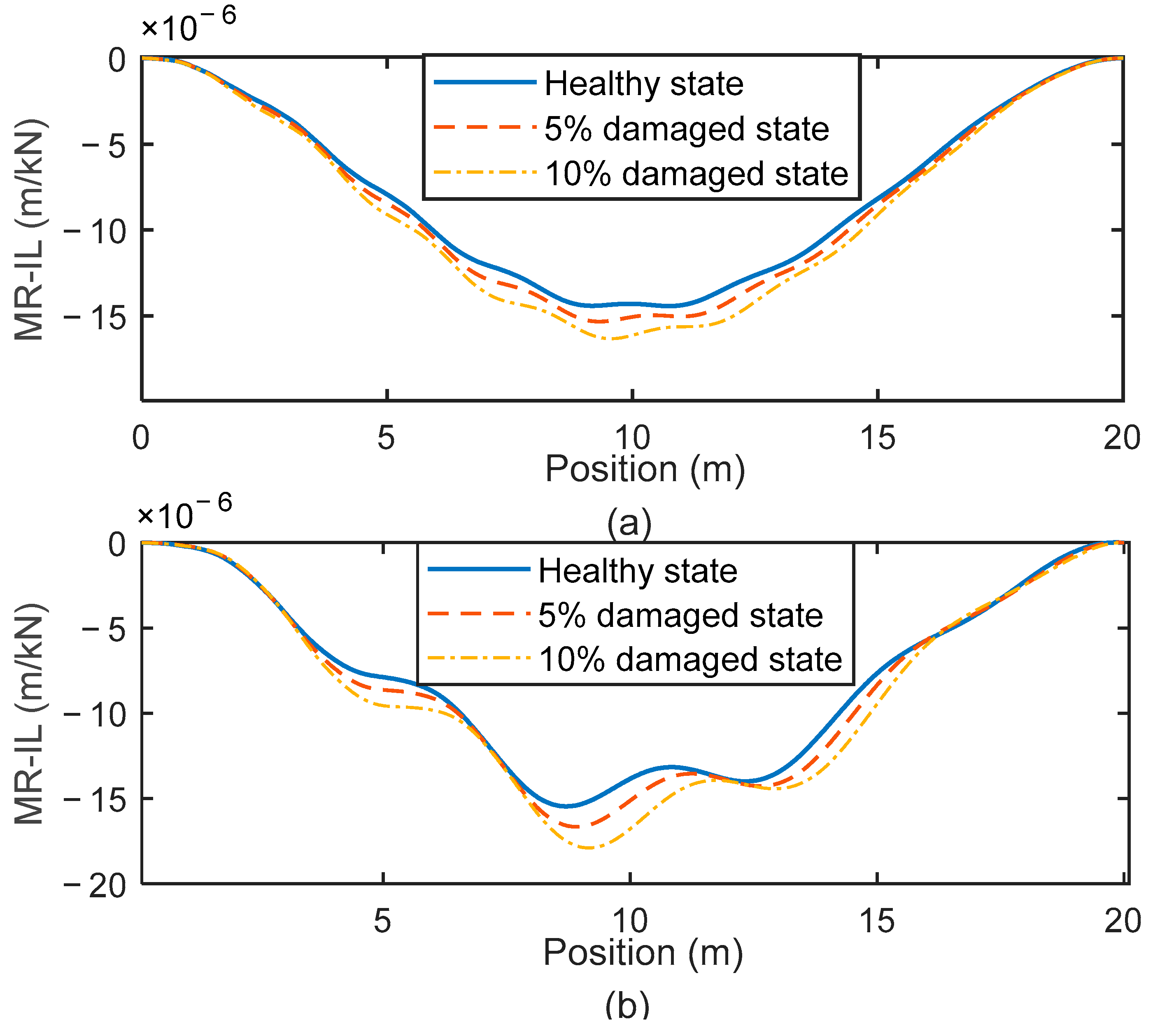
Two bridge states with different levels of global damage are simulated, with the resulting moving reference deflections and MR-ILs. It is acknowledged that the capacity of the bridge is different from its flexural rigidity (stiffness). However, the two are well correlated and changes in flexural rigidity are used here to simulate changes in bridge condition. The overall losses of flexural rigidity are 5% and 10%. Batches of 20 vehicles are generated with the same property values in Table 2 and simulated crossing the bridge in its healthy state and in the two damaged states. Two speeds are used separately: 10 m/s and 20 m/s. The mean calculated MR-ILs of the three bridge states are shown in Figure 8. The mean of the 20 mid-span MR-IL values, denoted $\widetilde{IL}$, is chosen as an indicator of bridge damage. It is noted that MR-IL is inversely proportional to the flexural rigidity, so it is inversely proportional to damage. For this reason, $Damage Indicator 1$is defined by Equation (24). The area under the mean calculated MR-ILs (denoted $I{L}^{*}$) is used as $Damage Indicator 2$.

$$\begin{gathered} Damage Indicator1\left(D1\right)=100\left\{1-\frac{{\left(\raisebox{1ex}{$1$}\!\left/ \!\raisebox{-1ex}{$\widetilde{IL}$}\right.\right)}^D}{{\left(\raisebox{1ex}{$1$}\!\left/ \!\raisebox{-1ex}{$\widetilde{IL}$}\right.\right)}^H}\right\}=100\left\{1-\frac{{\left(\widetilde{IL}\right)}^H}{{\left(\widetilde{IL}\right)}^D}\right\} \\ Damage Indicator 2 \left(D2\right)=100\left\{1-\frac{{\left(\raisebox{1ex}{$1$}\!\left/ \!\raisebox{-1ex}{$I{L}^{*}$}\right.\right)}^D}{{\left(\raisebox{1ex}{$1$}\!\left/ \!\raisebox{-1ex}{$I{L}^{*}$}\right.\right)}^H}\right\}=100\left\{1-\frac{{\left(I{L}^{*}\right)}^H}{{(I{L}^{*})}^D}\right\} \end{gathered}$$

(24)

The calculated damage indicator values are shown in

Table 3. Inferred damaged indicators and true damage levels.

True damage level		0%	5%	10%
10 m/s	$Damage Indicator 1$	0%	5%	11%
	$Damage Indicator 2$	0%	5%	10%
20 m/s	$Damage Indicator 1$ with filter	0%	5%	12%
	$Damage Indicator 1$ without filter	0%	7%	15%
	$Damage Indicator 2$	0%	5%	10%

. For this simple example, there is a clear strong correlation between the damage indicators and the true loss of flexural rigidity. For the high-speed case, $Damage Indicator 1$ is less accurate because of dynamic effects, though it can show the damage state. The mean calculated MR-ILs are passed through a low pass filter to remove the oscillation at the bridge frequency, which makes results better. Other filters may be appropriate for other examples; the filters used here were effective for this case. For other cases, it may, for example, be necessary to remove records at particular speeds. $Damage Indicator 2$ is an effective way to detect bridge damage, even with dynamic effects. In fact, bridge first natural frequency and other frequencies may influence the calculated MR-IL values. Nevertheless, this indicator can be used to detect the level of damage with reasonable accuracy.

6. Blind Tests

The concept of monitoring railway bridge condition using batches of instrumented trains was assessed in a series of blind tests. A team from the Norwegian University of Science and Technology (NTNU) used the advanced model described in Section 2 to simulate batches of train carriages crossing a railway track and a culvert. The vertical accelerations and angular velocities from two bogies were generated by NTNU for various cases of the bridge condition. University College Dublin (UCD) analysed these signals to calculate the AP, determine the train properties, and detect the bridge damage level using the methods described above.

In these tests, the ‘off-bridge’ length of track used for calibration was 120 m (unknown to UCD) and the length of the bridge was 10.2 m. Data were analysed for 7 different bridge damage states, including one perfectly healthy state. Global damage was simulated but, for each damaged bridge, there were small random differences (5% standard deviation) between element flexural rigidities (stiffnesses), reflecting the natural variation in a corroded bridge. For each state, data from 50 different train journeys were used. In each run, all properties were kept constant except for the local properties of mass ($m_v$), moment of inertia ($I_v$), and speed ($v$) (

Table 4. Carriage vehicle properties in the blind test.

Property	Type	Symbol	Unit	Value before Random Noise
Carriage body mass	Local	$m_v$	kg	Varied
Carriage body moment of inertia	Local	$I_v$	kg m2	Varied
Speed	Local	$v$	m/s	Varied
Bogie mass	Global	$m_b$	kg	2615
Bogie moment of inertia	Global	$I_b$	kg m2	1476
Wheelset mass	Global	$m_w$	kg	1813
Primary suspension stiffness	Global	$k_p$	N/m	2.4 × 106
Secondary suspension stiffness	Global	$k_s$	N/m	0.86 × 106
Primary suspension damping	Global	$c_p$	N s/m	7 × 103
Secondary suspension damping	Global	$c_s$	N s/m	16 × 103
Distance between bogie centre of gravity and wheelsets	Global	$L_b$	m	1.28
Distance between main body centre of gravity and bogies	Global	$L_v$	m	9.5

). For each batch of runs, NTNU used Monte Carlo simulation to randomly generate these properties for each of the 50 vehicles in the fleet. The individual vehicle local property values were not made known to UCD but the means were provided, on the basis that these mean values are repeatable and can be determined for a particular site. UCD was provided with the approximate speed ($v$) which was slightly different from the true value (to represent inaccuracy in a Global Positioning System (GPS) measurement). NTNU applied random noise (5% standard deviation) to other global vehicle properties when generating the signals to represent inaccuracy resulting from a global calibration process. Reference global property values were used by UCD, which is shown in Table 4.

For the railway track, variable stiffness at the ballast and sub-ballast levels were generated randomly using a ‘Gaussian process’ algorithm, which allows small incremental changes. To confirm that the method is not sensitive to the profile assumed, the entire process (healthy and 6 damage states) was repeated for two different track profiles, making a total of 14 batches of runs. To help establish the baseline, the two batches for which the bridge was healthy were identified to UCD as such. To separate the track and bridge parts, the starting point of the bridge in each run was provided. For application in the field, it is proposed that the location of the bridge relative to the data can be estimated with a GPS and can be found more accurately using an optimisation algorithm. In this blind test, UCD used the 4-axle railway carriage model and the 2-axle 2-degree-of-freedom half-car model to analyse these signals.

6.1. Results with 4-Axle Railway Carriage Model

The 4-axle railway carriage model used by UCD (Figure 1) is the same as that used by NTNU. Hence, the validation in this subsection does not address differences in the models. It does show the ability of the proposed approach to infer model parameter values from the simulated values provided by NTNU to UCD and an insensitivity to some potential sources of inaccuracy (vehicle global property values and bridge flexural rigidities).

Using the off-bridge data and the fleet monitoring concept, the APs and vehicle local properties (masses, moments of inertia, and speeds) were calculated from the vertical accelerations and angular velocities. Figure 9 shows the calculated AP from one run under the 1st axle over Profile 1. It is compared to the true AP, provided subsequently by NTNU. This result is for the bridge in State 7 (healthy), but this has no effect as the data are off-bridge. It shows an obvious difference between calculated AP and true AP in the initial value, which generates a constant difference in the whole signal. The calculated AP is shifted by the difference between the true and calculated AP at the start point (the 0 position). All the points of the calculated AP are shifted by subtracting this quantity. After shifting, there is a very close match between calculated APs after shifting and true APs. 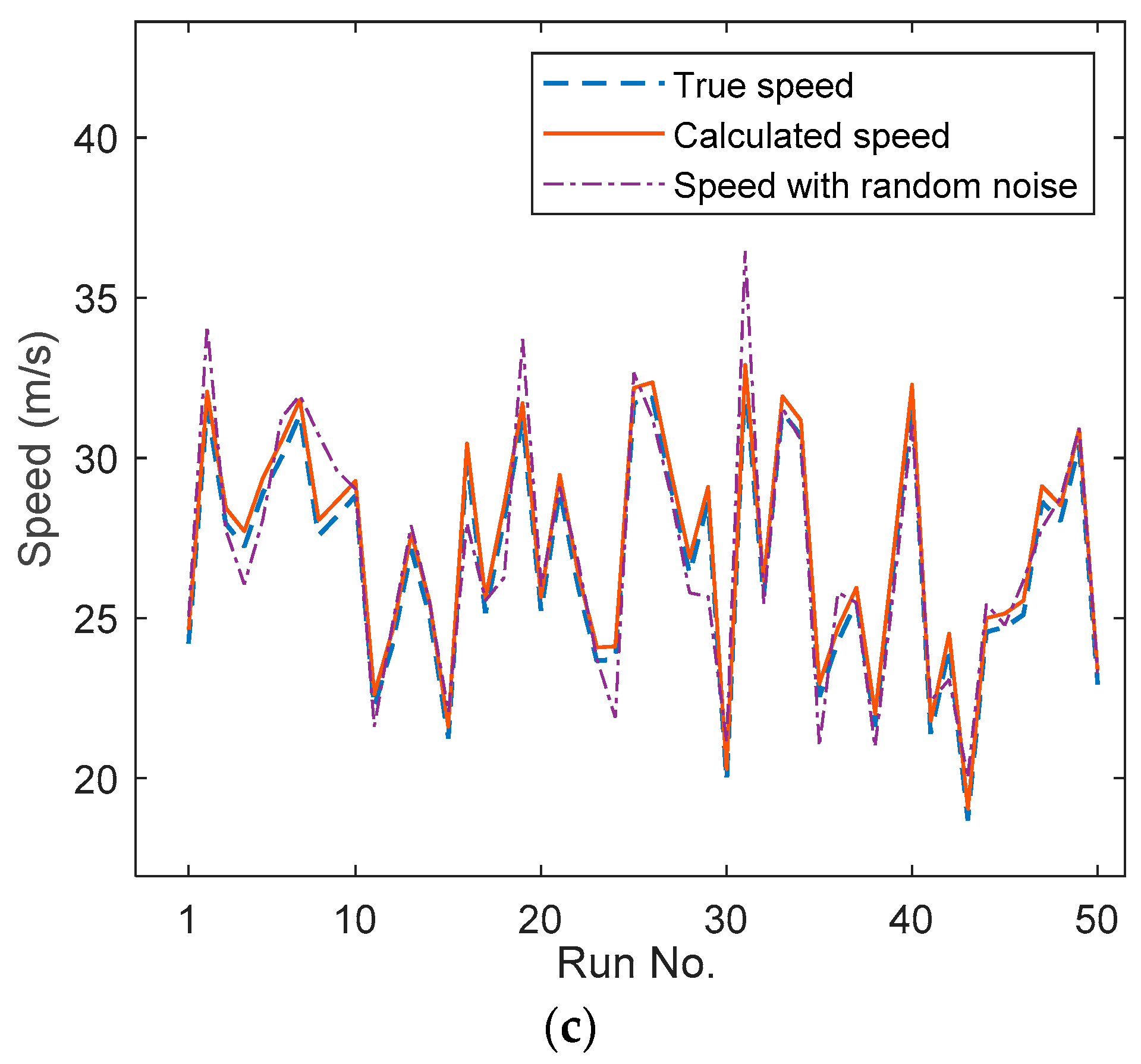Figure 10 shows the calculated values for the local vehicle properties for each of the 50 trains in the batch for Profile 1, State 7. The calculated vehicle properties are generally close to the true values, with some small differences for particular vehicles. As can be seen in Figure 10c, the speeds given by NTNU are sometimes significantly different from the true values (e.g., Run 2), but the calculated speeds are quite accurate.

The vehicle properties calculated using the off-bridge data are used to find the APs for the section of track on the bridge. For each run, the APs under each of the four wheels are found using the Inverse Newmark-β method from the signals provided by NTNU. The calculated AP of the bridge from one run over Profile 1, State 7, is shown in Figure 11. In this figure, the calculated AP is very close to the true one after shifting. The fundamental MR-IL of the first bogie is calculated from the APs under these two wheels using the method described in Section 5. 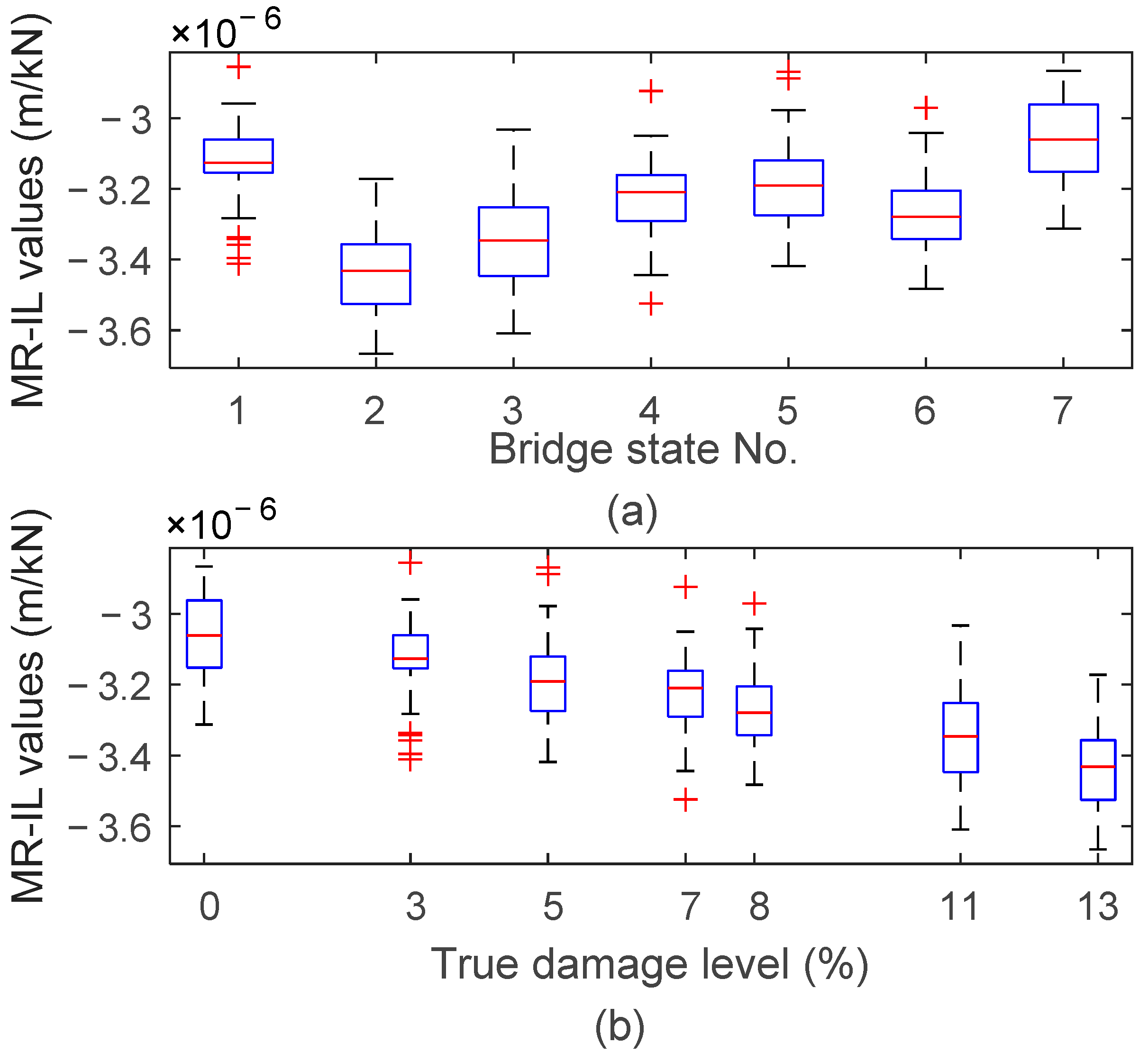Figure 12 presents box plots showing the mid-span MR-IL values for Profile 1 and different bridge damage states/damage levels. Each box represents data from 50 mid-span MR-IL values and one bridge state. Here, the State 7 is the healthy bridge and has the smallest MR-IL values. On each box, the central mark indicates the median, and the bottom and top edges of the box indicate the 25th and 75th percentiles, respectively. The whiskers extend to the most extreme data points not considered outliers, and the outliers are plotted individually using the ‘+’ symbol. The box plot shows that the mid-span MR-IL values provide good repeatability, with obvious differences between damage states. The mean of the 50 mid-span MR-IL values and the area under the mean calculated MR-IL is used to calculate the bridge damage indicator defined in Equation (24).

The corresponding true levels of damage, reported by NTNU, are defined as the percentage losses in flexural rigidity. The numerical results are presented in

Table 5. Inferred and true damage levels.

Bridge State No.			1	2	3	4	5	6	7
4-axle railway carriage model	Profile 1	$D1$	3%	12%	9%	6%	4%	7%	0%
		$D2$	4%	14%	11%	7%	5%	8%	0%
	Profile 2	$D1$	5%	11%	9%	7%	4%	7%	0%
		$D2$	5%	12%	10%	7%	5%	7%	0%
2-axle half-car	Profile 1	$D1$	4%	10%	9%	4%	2%	6%	0%
		$D2$	5%	11%	10%	4%	3%	6%	0%
	Profile 2	$D1$	3%	10%	8%	6%	5%	6%	0%
		$D2$	2%	9%	7%	5%	3%	6%	0%
True damage level			3%	13%	11%	7%	5%	8%	0%

$D1$ means $DamageIndicator1$ and $D2$ means $DamageIndicator2$.

. All damage states were identified, and the level of damage was accurately found, without prior knowledge of the true states. There is little sensitivity to the profile used in the simulations. Furthermore, there is little difference in the effectiveness of $Damage Indicator 1$ and $Damage Indicator 2$.

6.2. Results with 2-Axle Half-Car

UCD also used a 2-axle 2-degree-of-freedom half-car to represent the bogie of the NTNU 4-axle railway carriage model. The objective was to determine if the method is effective when the numerical model (of UCD) is simpler than the true behaviour (simulated by NTNU). The researchers attempt to create a situation where, as in real life, the model used in the damage calculation is less sophisticated than the model (or the reality) used to generate the input data to the algorithm. The 2-axle model has the capacity to capture the bouncing and rocking motions of the bogie but not the carriage rocking motion that transfers load between bogies.

For a 2-axle half-car, given the vertical accelerations and angular velocities, APs under each axle can be calculated using the Inverse Newmark-β integration scheme. Here, all the vehicle properties relate to the bogie and are global properties. The property values, before the application of random noise, are shown in

Table 6. Half car vehicle properties in the blind test.

Property	Symbol	Unit	Corresponding Property in 4-Axle Railway Carriage Model	Value
Sprung mass	$m_s$	kg	$m_b$	2615
Sprung mass moment of inertia	$I_s$	kg m2	$I_b$	1476
Spring stiffness	$K_1, K_2$	N/m	$K_p$	2.4 × 106
Damping	$C_1, C_2$	N s/m	$C_p$	7 × 103
Distance of axle to body centre of gravity	$D_1, D_2$	m	$L_b$	1.28

. Using the calculated APs under the two axles, the MR-ILs of each run are determined using the method described in Section 5. To calculate the MR-ILs, the 1st and 2nd axle weights, W_A and W_B, are determined from carriage mass, $m_v$, bogie mass, $m_b$, and wheelset mass, $m_w$. However, in this case, the individual carriage mass, $m_v$, for each run is not given. The mean value of $m_v$ is used to calculate axle weights.

A box plot showing the mid-span MR-IL values for Profile 1 is plotted in Figure 13. For this calculation, there is considerably more variability in the damage indicators for individual runs, relative to the differences due to damage. However, the calculated damage levels still compare well with the corresponding true levels, as shown in Table 5.

7. Conclusions

This article presents a numerical investigation of a novel method to determine AP and detect bridge damage using bogie vertical accelerations and angular velocities measured in batches of passing trains. Firstly, an Inverse Newmark-β method is developed to calculate the AP of the railway track using train accelerations. A 4-axle railway carriage and train/track/bridge dynamic interaction model is used here to generate vehicle bogie vertical accelerations and angular velocities, the simulated measurements. The result shows that the calculated AP is the same as the ‘true’ AP and this method is efficient. Combining the Inverse Newmark-β method with CE optimisation, the APs of the track and vehicle properties can be calculated accurately using batches of trains.

The work is expanded to introduce a new method to determine the moving reference influence line from moving reference deflections. A 2-axle half-car and track beam model is tested with different bridge damage levels. The results show that the moving reference influence line is a good indicator of the bridge damage level.

Finally, the results are validated in a blind test with an independent research group. For this, the analysis is carried out using the same 4-axle railway carriage model that generated the data and a simpler 2-axle half-car. For both cases, the moving reference influence lines are determined using measurements from the train. Furthermore, the damage levels of the bridge are inferred by the calculated moving reference influence lines with very good accuracy.

The idea of the fleet monitoring concept is developed in this article. As it will monitor the bridge through time, it will average out the effects through a variety of environmental conditions, including temperature. This mitigates against ‘contamination’ by changes in environmental conditions. The fleet monitoring concept has the potential to monitor bridges by combining drive-by data from a large number of in-service trains. To analyse large amounts of data, the fleet monitoring concept can be further developed using machine learning strategies. A passenger carriage is simulated here. It is expected that using freight carriages with one level of suspension would tend to improve the accuracy of the calculated AP. The train used in this article is modelled simply as a 2D model. Further work is needed to extend this to a 3D train model and to allow for non-linearity in the vehicle. Ultimately, field testing will be needed to validate the concept.

References

- Feng, K.; González, A.; Casero, M. A kNN algorithm for locating and quantifying stiffness loss in a bridge from the forced vibration due to a truck crossing at low speed. Mech. Syst. Signal Process. 2021, 154, 107599. [Google Scholar] [CrossRef]
- Majumder, L.; Manohar, C.S. A time-domain approach for damage detection in beam structures using vibration data with a moving oscillator as an excitation source. J. Sound Vib. 2003, 268, 699–716. [Google Scholar] [CrossRef]
- Hasni, H.; Jiao, P.; Lajnef, N.; Alavi, A.H. Damage localization and quantification in gusset plates: A battery-free sensing approach. Struct. Control Health Monit. 2018, 25, e2158. [Google Scholar] [CrossRef]
- Hasni, H.; Jiao, P.; Alavi, A.H.; Lajnef, N.; Masri, S.F. Structural health monitoring of steel frames using a network of self-powered strain and acceleration sensors: A numerical study. Autom. Constr. 2018, 85, 344–357. [Google Scholar] [CrossRef]
- Azim, M.R.; Gül, M. Damage detection of steel girder railway bridges utilizing operational vibration response. Struct. Control Health Monit. 2019, 26, e2447. [Google Scholar] [CrossRef]
- Weston, P.; Roberts, C.; Yeo, G.; Stewart, E. Perspectives on railway track geometry condition monitoring from in-service railway vehicles. Veh. Syst. Dyn. 2015, 53, 1063–1091. [Google Scholar] [CrossRef]
- Yang, Y.B.; Wang, Z.-L.; Shi, K.; Xu, H.; Wu, Y.T. State-of-the-art of the vehicle-based methods for detecting the various properties of highway bridges and railway tracks. Int. J. Struct. Stab. Dyn. 2020, 20, 2041004. [Google Scholar] [CrossRef]
- ISEN13848. Railway Applications-Track-Track Geometry Quality—Part 2: Measuring Systems—Track Recording Vehicles; CEN European Committee for Standardisation: Brussels, Belgium, 2018. [Google Scholar]
- Cantero, D.; Basu, B. Railway infrastructure damage detection using wavelet transformed acceleration response of traversing vehicle. Struct. Control Health Monit. 2015, 22, 62–70. [Google Scholar] [CrossRef]
- OBrien, E.J.; Bowe, C.; Quirke, P.; Cantero, D. Determination of longitudinal profile of railway track using vehicle-based inertial readings. Proc. Inst. Mech. Eng. Part F J. Rail Rapid Transit 2016, 231, 518–534. [Google Scholar] [CrossRef] [Green Version]
- Yang, Y.B.; Wang, Z.L.; Wang, B.Q.; Xu, H. Track modulus detection by vehicle scanning method. Acta Mech. 2020, 231, 2955–2978. [Google Scholar] [CrossRef]
- Tsunashima, H.; Naganuma, Y.; Matsumoto, A.; Mizuma, T.; Mori, H. Condition monitoring of railway track using in-service vehicle. Reliab. Saf. Railw. 2012, 12, 334–356. [Google Scholar]
- Kobayashi, T.; Naganuma, Y.; Tsunashima, H. Condition monitoring of shinkansen tracks based on inverse analysis. Chem. Eng. Trans. 2013, 33, 703–708. [Google Scholar]
- Ren, Y.; Keenahan, J.; O’Brien, E.J. A two-stage direct integration approach to find the railway track profile using in-service trains. In Proceedings of the The 2020 Civil Engineering Research in Ireland Conference, Cork, Ireland, 27–28 August 2020. [Google Scholar]
- O’Brien, E.J.; Quirke, P.; Bowe, C.; Cantero, D. Determination of railway track longitudinal profile using measured inertial response of an in-service railway vehicle. Struct. Health Monit. 2017, 17, 1425–1440. [Google Scholar] [CrossRef]
- Real, J.; Salvador, P.; Montalbán, L.; Bueno, M. Determination of rail vertical profile through inertial methods. Proc. Inst. Mech. Eng. Part F J. Rail Rapid Transit 2010, 225, 14–23. [Google Scholar] [CrossRef]
- Wei, X.; Liu, F.; Jia, L. Urban rail track condition monitoring based on in-service vehicle acceleration measurements. Measurement 2016, 80, 217–228. [Google Scholar] [CrossRef]
- Paixao, A.; Fortunato, E.; Calcada, R. Smartphone’s sensing capabilities for on-board railway track monitoring: Structural performance and geometrical degradation assessment. Adv. Civ. Eng. 2019, 2019, 1729153. [Google Scholar] [CrossRef]
- Yang, Y.B.; Yang, J.P. State-of-the-Art review on modal identification and damage detection of bridges by moving test vehicles. Int. J. Struct. Stab. Dyn. 2018, 18, 1850025. [Google Scholar] [CrossRef]
- Malekjafarian, A.; McGetrick, P.J.; O’Brien, E.J. A review of indirect bridge monitoring using passing vehicles. Shock Vib. 2015, 2015, 286139. [Google Scholar] [CrossRef] [Green Version]
- Kim, C.W.; Isemoto, R.; McGetrick, P.J.; Kawatani, M.; O’Brien, E.J. Drive-by bridge inspection from three different approaches. Smart Struct. Syst. 2014, 13, 775–796. [Google Scholar] [CrossRef] [Green Version]
- Kong, X.; Cai, C.S.; Deng, L.; Zhang, W. Using dynamic responses of moving vehicles to extract bridge modal properties of a field bridge. J. Bridge Eng. 2017, 22, 04017018-1-11. [Google Scholar] [CrossRef]
- Yang, Y.B.; Lin, C.W.; Yau, J.D. Extracting bridge frequencies from the dynamic response of a passing vehicle. J. Sound Vib. 2004, 272, 471–493. [Google Scholar] [CrossRef]
- Zhang, Y.; Wang, L.; Xiang, Z. Damage detection by mode shape squares extracted from a passing vehicle. J. Sound Vib. 2012, 331, 291–307. [Google Scholar] [CrossRef]
- Yang, Y.B.; Zhang, B.; Chen, Y.; Qian, Y.; Wu, Y. Bridge damping identification by vehicle scanning method. Eng. Struct. 2019, 183, 637–645. [Google Scholar] [CrossRef]
- O’Brien, E.J.; Keenahan, J. Drive-by damage detection in bridges using the apparent profile. Struct. Control Health Monit. 2015, 22, 813–825. [Google Scholar] [CrossRef] [Green Version]
- Elhattab, A.; Uddin, N.; O’Brien, E.J. Drive-by bridge damage monitoring using Bridge Displacement Profile Difference. J. Civ. Struct. Health 2016, 6, 839–850. [Google Scholar] [CrossRef]
- Keenahan, J.C.; O’Brien, E.J. Drive-by damage detection with a TSD and time-shifted curvature. J. Civ. Struct. Health 2018, 8, 383–394. [Google Scholar] [CrossRef]
- Quirke, P.; Bowe, C.; O’Brien, E.J.; Cantero, D.; Antolin, P.; Goicolea, J.M. Railway bridge damage detection using vehicle-based inertial measurements and apparent profile. Eng. Struct. 2017, 153, 421–442. [Google Scholar] [CrossRef]
- Fitzgerald, P.C.; Malekjafarian, A.; Cantero, D.; O’Brien, E.J.; Prendergast, L.J. Drive-by scour monitoring of railway bridges using a wavelet-based approach. Eng. Struct. 2019, 191, 1–11. [Google Scholar] [CrossRef]
- Rakoczy, A.M.; Otter, D.E.; Malone, J.J.; Farritor, S. Railroad bridge condition evaluation using onboard systems. J. Bridge Eng. 2016, 21, 04016044-1-12. [Google Scholar] [CrossRef]
- Rakoczy, A.M.; Shu, X.; Otter, D. Vehicle–track–bridge interaction modeling and validation for short span railway bridges. Transp. Res. Rec. J. Transp. Res. Board 2017, 2642, 127–138. [Google Scholar] [CrossRef]
- Micu, A.E.; O’Brien, E.J.; Bowe, C.; Fitzgerald, P.; Pakrashi, V. Bridge damage and repair detection using an instrumented train. J. Bridge Eng. 2022, 27, 1–12. [Google Scholar] [CrossRef]
- Cantero, D.; Arvidsson, T.; O’Brien, E.J.; Karoumi, R. Train–track–bridge modelling and review of parameters. Struct. Infrastruct. E 2016, 12, 1051–1064. [Google Scholar] [CrossRef]
- Lei, X.; Noda, N.A. Analyses of dynamic response of vehicle and track coupling system with random irregularity of track vertical profile. J. Sound Vib. 2002, 258, 147–165. [Google Scholar] [CrossRef]
- Lou, P. Finite element analysis for train–track–bridge interaction system. Arch. Appl. Mech. 2007, 77, 707–728. [Google Scholar] [CrossRef]
- Nguyen, G.K.; Goicolea, R.M.; Gabaldon, C.F. Comparison of dynamic effects of high-speed traffic load on ballasted track using a simplified two-dimensional and full three-dimensional model. Proc. Inst. Mech. Eng. Part F J. Rail Rapid Transit 2012, 228, 128–142. [Google Scholar] [CrossRef]
- Lu, F.; Kennedy, D.; Williams, F.W.; Lin, J.H. Symplectic analysis of vertical random vibration for coupled vehicle–track systems. J. Sound Vib. 2008, 317, 236–249. [Google Scholar] [CrossRef]
- Zhai, W.M.; Wang, K.Y.; Lin, J.H. Modelling and experiment of railway ballast vibrations. J. Sound Vib. 2004, 270, 673–683. [Google Scholar] [CrossRef]
- Keenahan, J.; Ren, Y.; OBrien, E.J. Determination of road profile using multiple passing vehicle measurements. Struct. Infrastruct. E 2020, 16, 1262–1275. [Google Scholar] [CrossRef]
- Rubinstein, R.Y.; Kroese, D.P. The Cross-Entropy Method: A Unified Approach to Combinatorial Optimization, Monte-Carlo Simulation and Machine Learning; Springer: New York, NY, USA, 2004. [Google Scholar]
- Botev, Z.; Kroese, D.P. Global likelihood optimization via the CE method, with an application to mixture models. In Proceedings of the 36th Conference on Winter Simulation, Washington, DC, USA, 5–8 December 2004; pp. 529–535. [Google Scholar]
- O’Brien, E.J.; Quilligan, M.; Karoumi, R. Calculating an influence line from direct measurements. Proc. Inst. Civ. Eng. Bridge Eng. 2006, 159, 31–34. [Google Scholar] [CrossRef]
- Iwnicki, S. Manchester benchmarks for rail vehicle simulation. Veh. Syst. Dyn. 1998, 30, 295–313. [Google Scholar] [CrossRef]
- Gonzalez, A.; O’Brien, E.J.; McGetrick, P.J. Identification of damping in a bridge using a moving instrumented vehicle. J. Sound Vib. 2012, 331, 4115–4131. [Google Scholar] [CrossRef] [Green Version]
Figure 1.
Two-dimensional (2D) 4-axle railway carriage model.
Figure 3.
(a) Elevation of track-bridge model. (b) Detail of track-bridge model of (a).
Figure 4.
‘True’ AP and calculated AP using the Inverse Newmark-β equations.
Figure 5.
Deflection responses to moving unit load: (a) Response at x to load at x; (b) Response at x to load at y.
Figure 6.
(a) 2-degree-of-freedom half-car and beam model; (b) 2-degree-of-freedom half-car model.
Figure 7.
True and calculated fundamental MR-ILs for bridge and vehicle at different speeds: (a) 2 m/s; (b) 10 m/s; (c) 20 m/s.
Figure 8.
Mean calculated MR-ILs with different damage at different speed: (a) 10 m/s; (b) 20 m/s.
Figure 9.
Calculated AP, calculated AP after shifting, and true AP (off-bridge) for Profile 1, State 7, and Run No. 1.
Figure 10.
(a). Calculated vehicle masses for each of the 50 runs in the batch, running on Profile 1, State 7. (b). Calculated vehicle moments of inertia for each of the 50 runs in the batch, running on Profile 1, State 7. (c) Calculated vehicle speeds for each of the 50 runs in the batch, running on Profile 1, State 7.
Figure 11.
The true and calculated AP of the bridge from one run over Profile 1, State 7.
Figure 12.
Box plot of mid-span fundamental MR-IL values of carriage model for Profile 1, organised by (a) bridge state number and (b) damage level.
Figure 13.
Box plot of mid-span fundamental MR-IL values of half-car model for Profile 1, organised by (a) bridge state number and (b) damage level.