A Hybrid Approach for an Efficient Estimation and Control of Permanent Magnet Synchronous Motor with Fast Dynamics and Practically Unavailable Measurements

Abstract

This paper presents an interesting hybrid solution to a challenging estimation and control problem of the Permanent Magnet Synchronous Motor (PMSM). Apart from the inherently nonlinear nature of the PMSM, which makes this problem particularly challenging, is the unavailability of the measurements, rotor position, and speed. In an effort to efficiently cope with such issues along with the random noise environment, the Unscented Kalman Filter (UKF) is chosen to estimate the states of the PMSM dynamic system and the Model Predictive Control (MPC) is utilized to control the state space vector in Pulse Width Modulation (PWM). Additionally, the MPC has also been implemented in combination with the Extended Kalman Filter (EKF) and also with Sliding Mode Control (SMC), in order to vigorously compare these hybrid approaches in terms of accuracy, robustness, and transient response. The MPC-UKF, a combination that has never been implemented before, outperforms the other two by efficiently dealing with the issues of high nonlinearities, by accurately estimating the states while the measurements were practically unavailable, and coping with the fast dynamics of the PMSM.

1. Introduction

In recent years, power electronics and modern control designs are emerging widely which boost the use of Permanent Magnet Synchronous Motors (PMSM). The PMSM is extensively used in various fields due to multi-facet benefits, such as high dynamic speed, high torque, good efficiency, low maintenance cost, reliable operation, and simple structure. In motors, to achieve perfect commutation, signals after every 60 electrical degrees need to be computed to estimate position and speed. For this purpose, sensors on the rotors are used, such as photovoltaic and hall sensors [1]. However, sensors require additional space, leading to an overall increase in size and cost with frequent maintenance. Therefore, to eliminate such problems, sensorless control technology suddenly received great attention from researchers [2].

In PMSM, for sensorless control, observers are designed to estimate such states/parameters that cannot be measured directly or through other available states. There are many techniques available for estimating the motor parameters to control the motor. Problems associated with estimation techniques without sensors include inaccuracy at low speed, disturbance rejection, poor dynamic performance, constraint handling with safer starting conditions, and switching losses of the inverter due to high switching frequency [3].

In PMSM, the sensorless estimation techniques are categorized as: (a) adaptive methods, (b) non-adaptive methods, (c) signal injection methods, and (d) artificial intelligence methods [4,5,6]. The non-adaptive methods include stator current and stator voltage estimators, flux-based estimators, back EMF estimators, and DC link methods [7]. Moreover, there are several sub-groupings of adaptive methods, such as Luenberger-based observers, Model Reference Adaptive (MRAS) estimators, Kalman-based stochastic filters, and sliding mode observers [8]. All these techniques are mature enough to achieve the maximum optimal results.

Table 1. Comparative Literature Survey on State-of-the-Art Techniques.

Techniques	Types	Benefits	Drawbacks
	Direct calculation [4]	Fast, dynamic, and Simple	Parametric variation error
Open Loop	Determination of stator inductance [5]	Zero speed estimation	Inaccurate at high stator current, valid for salient motors
	Back EMF integration [7]	Fast, Robust, and accurate at high frequency	Difficult to calculate back EMF, not accurate at low speeds
	EKF [9]	Reduced computation time and noise rejection	Low speed, poor performance
Closed Loop	MRAS [10]	Adaptation at high speed, machine model not required	Parametric sufferance
	SMO [11]	Robust, parametric invariance and no steady state error	Stand still or zero speed performance is poor
	Low Frequency injection [12]	Applicable even for non-salient motors	Dynamic performance is poor, saturation problem
Non-ideal property-based	High Frequency injection [13]	Coordinate transformation not required	Not applicable for higher inertia motor, slow dynamic response
	INFORM [14]	Parameter invariance	Flux distortion and current ripples cause estimation error

illustrates the limitations and benefits of all sensorless estimation techniques.

The Kalman Filter (KF) is an optimal state estimator but only for linear systems because the update rule of the KF makes optimal decisions based only on the first two instants of states viz. mean and covariance. Therefore, the cases where the system is nonlinear, the KF does not provide optimal results because of non-Gaussian noise. However, a modified form of the KF is the Extended Kalman Filter (EKF), in which transformation from nonlinear to linear is done via the Jacobian matrix that makes the calculations simpler but less accurate. In the case of highly nonlinear systems, linearization results in bad performance [15].

Approximation issues of the EKF are addressed in the Unscented Kalman Filter (UKF) formulation. The Unscented Transformation (UT) is used in the UKF process instead of linearization approach. Gaussian Random Variable (GRV) represents the state distribution of both the algorithms; however, in UKF minimum sample points are carefully chosen. The UT is used to calculate mean and covariance, which further helps find sigma points as accuracy is proportional to the number of sigma points [16]. The sigma points propagated through the true nonlinear function captures the true mean and covariance of the GRV. This process accurately estimates the posterior mean and covariance for any nonlinearity up to 2nd order.

The Model Predictive Control (MPC) is one of the widely used predictive control methods. In MPC, the optimal control and control instructions are obtained by a specific objective function that is determined through the mathematical model of the controlled object. In MPC, the cost function, system nonlinearities, and constraints can easily be considered and controlled by the Finite Control Set-Model Predictive Control (FCS-MPC). Inverters switching states are used to optimize the observer states of the motors and the FCS-MPC can efficiently handle the discrete nature of the switching states in the microprocessor [17].

In modern state estimation techniques of the motors, hybrid methodologies are employed by combining any of the two previous matured techniques. Szabat et al. described the application of UKF and Fuzzy UKF (FUKF) with an elastic connection for the estimation of parameters and mechanical state variables of the AC drives [18]. A suitable adaptation mechanism with IP controller reinforced by two supplementary feedbacks in the form of a cascade control structure is inspected [18]. However, the control structure performance degrades by the existing estimation error. Introduced hybrid modification improves the quality of the estimation. A fuzzy system has been designed based on linguistic rules. The authors reported better performance of the FUKF compared to the UKF; however, the former one requires pre-feed data of motors’ nonlinear behavior.

Wang et al. introduced a novel technique for the surface-mounted type of PMSM drives called Hybrid Dual-Mode Control (HDMC) that contains two control modes to find appropriate performances of the steady-state and transient response [19]. The HDMC is a hybrid combination of two techniques, which inherits the excellent steady-state routines of the Field Oriented Control (FOC) and the quick responsibility of the Deadbeat Predictive Control (DBPC).

The combination of MPC-EKF has been tested previously; however, Borsje et al. suggested that UKF has a remarkable advantage over EKF [7]. The PMSM model is highly nonlinear, and states’ estimation without sensors involves complexity in implementation due to noisy signals of the PWM [20]. The MPC handles the selection of the proper sequence of states for the inverter; therefore, the MPC increases efficiency and reduces time compared to the FOC method. Moreover, the MPC has many advantages, such as easy modeling, simple principle, constraints handling, and strong robustness [21]. Similarly, the UKF is very robust against parametric variation and handles the measurement noise and system noise. Optimal estimation of the states in Kalman filters is based on least-squares techniques.

In sensorless motor drive control, there is a significant impact of parametric variation, inverter nonlinearities, and zero/low-speed operation on the stability of the control system. Moreover, in a high-speed region, a high observer’s bandwidth is required. Various other issues, such as parametric variation, low back EMF, saturation problem, flux distortion, current ripples, and input constraint handling, create hindrance in the accurate estimation of position and speed. Therefore, by keeping in view all the aforementioned attributes, a novel MPC-UKF control scheme is proposed for the sensorless control of PMSM. In UKF, the unscented transformation technique has many advantages over the other observers, namely, finding the initial value and hassle-free tuning. The UKF is a derivative-free approach and does not require any linearization steps, so no Jacobean is needed. As the error of the motor parameters is considered at the beginning, the UKF-based speed and flux observation have strong robustness to motor parameters. The UKF acts as an observer because of its simplicity of two-step procedures: prediction and correction. Moreover, it estimates the parameters even at a relatively low speed that cannot be estimated with other controllers. According to the operation frequency, there are two main types of sensorless motor control: one is the model-based method that detects the fundamental component of back EMF. The other injects an additional excitation signal to utilize the asymmetrical effect of the inductance in PMSM. The first method works well in the high-speed range but fails at low speed when the signal-to-noise ratio (SNR) of the EMF is too small for observation. On the contrary, the second method can derive position at low and even zero speed but performs poorly at high speed due to the limitation of observer bandwidth. To achieve a whole-speed-range of sensorless operation, a hybrid position estimation strategy combining both methods at middle speed is adopted. Two variables describe the UKF states: an estimate of the current state’s derivative is based on the knowledge of observation and error covariance matrix, that is, the uncertainty of the observation in the estimation process. The benefit of using MPC can be justified since in UKF, there are small errors during dynamical working caused by inaccurate modeling of the inverter, which is non-linear, and MPC also handles the gates switching very efficiently within defined constraints. The main contributions of the paper are:

• A hybrid approach, MPC-UKF, is tuned to a challenging PMSM control and estimation problem in order to efficiently deal with the issues of fastly varying dynamics, severe nonlinearities, random uncertainties, and unavailability of measurements [22].
• The MPC and the UKF are efficient control and estimation algorithms, respectively, and extension of these as a combination creates a novel solution to the challenges. Parametric invariance, disturbance rejection, and improved accuracy and estimates are the advantages of our proposed novel hybrid technique [23].
• In an effort to closely replicate the practical PMSM dynamics and to have more realistic findings with respect to the actual experimental setup, the practical factors, such as disturbances and uncertainties, process and measurement noise, have been taken into account. Such efforts certainly allow the observer, the UKF, to provide more accurate estimates that are otherwise sacrificed due to inappropriate, inaccurate, or incomplete system information. The UKF is successfully tuned to estimate speed and position of PMSM based on the direct available states, currents, and voltages.
• The MPC-UKF approach is compared with the combination of the MPC with state-of-the-art observer technique, the Sliding Mode Observer (SMO), and also with the more traditional approach, the EKF, in terms of robustness and reliability.

The remainder of the paper is organized as follows: Section 2 describes the mathematical modeling of the PMSM and discrete version of the model. Description of the control structure in the proposed scheme is presented in Section 3. Simulation results and discussions are presented in Section 4. The paper is concluded in Section 5 along with future directions.

2. Modeling of Permanent Magnet Synchronous Motor

A discrete model of the PMSM is necessary for the application of the proposed scheme. The synchronous $\mathit{dq}$-reference frame fixed to the rotor flux is derived for the said model since this scheme is more suitable than the $\alpha \beta$-reference frame. The major disadvantage of using the $\alpha \beta$-reference frame is that the UKF may converge to the wrong solution. The prediction steps might maintain the wrong solution and constantly update the estimation difference between actual and estimated voltages and currents. Wrong convergence of the solution may be avoided by a dedicated algorithm or by the hit-and-trial method [24]. However, $\mathit{dq}$-frame reference voltage equations avoid the wrong convergence solution because the equations do not fit. Therefore, using the $\mathit{dq}$-frame reference, a wrong startup is avoided. However, in the $\mathit{dq}$-frame reference, the coordinate transformation uses an estimated position. If the estimated position is wrong, then it may generate a constant error, which is a disadvantage of the $\mathit{dq}$-reference model. The PMSM has magnetic saliency with axial inductances $L_d$ and $L_q$. The notations used in the paper are listed in

Table 2. Notations used in the System Model.

Notation	Description	Notation	Description
$B_{\omega }$	Damping coefficient	$f\left(\theta \right)$	Normalized trapezoidal function
${\epsilon }_{a,b,c}$	RMS value of phase back EMF	${\stackrel{⏜}{\omega }}_r,{\omega }_r^{*}$	Estimated speed and reference speed
$i_{a,b,c},v_{a,b,c}$	Phase armature current and Phase Terminal Voltages	$i_{d,q}^{*},\stackrel{⏜}{\theta }$	Updated currents and Estimated position
$i_d,i_q$	Direct-axis and Quadrature-axis currents	${\mathbf{u}}_s$	Synchronous rotating frame stator voltage
$v_d,v_q$	Direct axis and Quadrature axis voltages	$S_{a,b,c}$	State space vectors
$v_n$	Neutral voltage	${\mathbf{i}}_s$	Synchronous rotating frame stator current vector
${\mathbf{i}}_{sm},{\mathbf{u}}_{sm}$	Current and voltage constraints	$e_s,i_{sm}$	Current predictive error and Current predictive vector value
$J,\rho$	Inertia of the rotor and number of poles	$\mathbf{h},\chi$	Correction factor and Sigma point matrix
$L_{a,b,c},M$	Phase self-inductance and Mutual Inductance	$\lambda ,P$	Scaling parameter and Covariance matrix
$L_d,L_q$	d-axis and q-axis magnetizing inductances	$\alpha$	Spread of sigma points around the mean
$R_s,T_s$	Phase resistance and Sampling Time	k	Secondary scaling parameter
$T_e,T$	Motor electromagnetic and loading torques	$W_i^m,W_i^c$	Weights for mean and covariance
$\theta$	Rotor position angle or position	$\overline{{\stackrel{⏜}{x}}^k},{\stackrel{⏜}{\mathbf{P}}}^k$	Predicted mean and predicted covariance
${\varphi }_f$	Amplitude of stator permanent magnet flux linkage	$Y_i^k$	Transformed sigma points in measurement space
${\omega }_e,{\mu }_0$	Electrical velocity and Permeability in air gap	$\overline{{\stackrel{⏜}{y}}^k}$	Mean in measurement space
${\mathbf{Q}}_{MPC},$${\mathbf{R}}_{MPC}$	Error and control weighting coefficient matrics	${\varphi }^k,{\mathbf{K}}^k$	Jacobian of the matrix and Kalman gain
${\mathbf{Q}}^k,{\mathbf{R}}^k$	Covariance matrices for process and measurement noises	${\mathbf{P}}_{yy}^k$	Predicted covariance matrix
${\mathbf{w}}^k,v^k$	Process noise vector and Measurement noise vector	${\mathbf{P}}_{xy}^k$	Cross-correlation matrix between actual and predicted spaces
$I_m$	Maximum rotor current	${\mathbf{P}}_{yy}^k$	Function that maps our sigma points to measurement space
$K_{\tau },K_{\epsilon }$	Torque constant and Back EMF constant	${\mathbf{P}}_{yy}^k$	Covariance in measurement space

where boldface letters show the vectors and matrices while lightface letters represent the scalar values. The PMSM’s mathematical model in continuous time frame is given as [25]:

$$\begin{array}{c}\hfill \frac{d{i}_d}{dt}=\frac{1}{L_d}(-R_s{i}_d+\frac{1}{2}\rho {\omega }_m{L}_q{i}_q+v_d)\end{array}$$

(1a)

$$\begin{array}{c}\hfill \frac{d{i}_q}{dt}=\frac{1}{L_q}(-R_s{i}_q-\frac{1}{2}\rho {\omega }_m{L}_d{i}_d+v_q-\frac{1}{2}\rho {\omega }_m{\varphi }_f)\end{array}$$

(1b)

$$\begin{array}{c}\hfill \frac{d{\omega }_m}{dt}=\frac{1}{J}(T_e-B_{\omega }{\omega }_m-T_l)\end{array}$$

(1c)

$$\begin{array}{c}\hfill \frac{d\theta }{dt}={\omega }_m\end{array}$$

(1d)

where $\frac{d{T}_l}{dt}\approx 0$ and electromechanical torque, $T_e=\frac{3}{2}\rho \left[{\varphi }_f{i}_q+(L_d-L_q)i_d{i}_q\right]$. Simplified assumptions are made to quickly evaluate the system performance, such as hysteresis and eddy currents losses are neglected, electromagnetically induced forces are sinusoidal, a saturation of magnetic material is zero, and airgap with no dynamical dependencies. In electromechanical torque, the $\frac{3}{2}$ is the frame conversion constant, and the change in load torque for the given sample time is zero. The Taylor series expansion is used for the discretization of each state variable given in the mathematical model of PMSM as [26]:

$$\begin{array}{c}\hfill x_j^{k+1}=x_j^k+{\left.\sum _{l=0}^{Nj}\frac{T_s^l}{l!}\frac{d^l{x}_j}{d{t}^l}\right|}_{tk}\end{array}$$

(2)

where $Nj$ is the number of expansion elements in the series normally used up to 1st order, and j is the number of state variables. Inputs of the system that appear in the discrete model affect the state variables, and each state is updated by the successive iteration that improves the accuracy. The discretization of the PMSM model is as follows [27]:

$$\begin{array}{c}\hfill i_d^{k+1}=i_d^k+\frac{1}{L_d}\left(-R_s{i}_d^k+{\omega }_e^k{L}_q{i}_q^k+v_d^k\right)T_s\end{array}$$

(3a)

$$\begin{array}{c}\hfill i_q^{k+1}=i_q^k+\frac{1}{L_d}\left(-R_s{i}_q^k-{\omega }_e^k{L}_d{i}_d^k+v_q^k-{\omega }_e^k{\varphi }_f\right)T_s\end{array}$$

(3b)

$$\begin{array}{c}\hfill T_e^{k+1}=\frac{3}{2}P\left({\varphi }_f{i}_q^{k+1}+\left(L_d-L_q\right)i_d^{k+1}{i}_q^{k+1}\right)\end{array}$$

(3c)

The matrix representation of the nonlinear discrete-time PMSM model used in the proposed scheme is [5]:

$$\begin{array}{c}\hfill {\mathbf{x}}^{k+1}={\mathbf{F}}^k{\mathbf{x}}^k+{\mathbf{B}}^k{\mathbf{u}}^k+w^k\end{array}$$

(4a)

$$\begin{array}{c}\hfill {\mathbf{y}}^k={\mathbf{H}}^k{\mathbf{x}}^{k+1}+v^k\end{array}$$

(4b)

with

$$\begin{array}{c}\hfill {\mathbf{F}}^k\left({\mathbf{x}}^k\right)=\left[\begin{array}{cccc}1-T_s·\frac{R_s}{L_d}& T_s·{\omega }_m\frac{L_q}{L_d}& 0& 0\\ -T_s·{\omega }_m\frac{L_q}{L_d}& 1-T_s·\frac{R_s}{L_q}& -T_s·\frac{{\varphi }_f}{L_q}& 0\\ 0& T_1& 0& 0\\ 0& 0& T_s& 1\end{array}\right],\end{array}$$

$$\begin{array}{cc}\hfill T_1& =\frac{3}{2}{T}_s·\frac{\rho }{J}\left[{\varphi }_f-\left(L_q-L_d\right)i_d\right],\hfill \\ \hfill {\mathbf{H}}^k\left({\mathbf{x}}^k\right)& =\left[\begin{array}{cccc}1& 0& 0& 0\\ 0& 1& 0& 0\end{array}\right],\hfill \\ \hfill \mathrm{and}{\mathbf{B}}^k\left({\mathbf{x}}^k\right)& =\left[\begin{array}{cc}{T}_s·\frac{1}{L_d}& T_s·\frac{1}{L_d}\\ -T_s·\frac{1}{L_q}& T_s·\frac{1}{L_q}\\ 0& 0\\ 0& 0\end{array}\right]\hfill \end{array}$$

The $i_q$ is the torque-producing component of the stator current and $i_d$ is flux-producing component of the stator current. When $i_q=I_m$, then $i_d=0$, which is a condition for maximum torque. The angle $\alpha$ between $i_q$ and $i_d$ determines the minimum and maximum torque computed as $\alpha ={tan}^{-1}\left(\frac{i_q}{i_d}\right)$. The $\alpha$ is the angle that determines the rotor position to compute the torque. Non-Gaussian noise as measurement noise $v^k$ and process noise $w^k$ are also added in the mathematical model for the real-time realization of the mathematical model. Moreover, it is also assumed to have very slow change in load torque compared to the sampling time. The state variables vector, input vector, and output vectors are as follows, respectively [5]:

$$\begin{array}{c}\hfill {\mathbf{x}}^k={\left[\begin{array}{cccc}{i}_d^k& i_q^k& {\omega }_m^k& {\theta }^k\end{array}\right]}^T\end{array}$$

(5a)

$$\begin{array}{c}\hfill {\mathbf{u}}^k={\left[\begin{array}{cc}{v}_d^k& v_q^k\end{array}\right]}^T\end{array}$$

(5b)

$$\begin{array}{c}\hfill {\mathbf{y}}^k={\left[\begin{array}{cc}{i}_d^{k+1}& i_q^{k+1}\end{array}\right]}^T\end{array}$$

(5c)

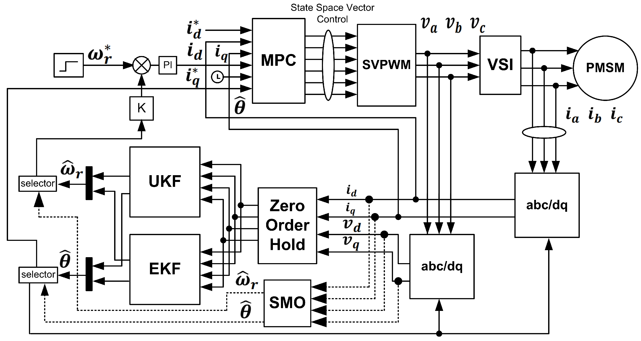
3. Description of Control Schemes

In this section, first, the mathematical model for the MPC is derived, then the MPC-SMO hybrid combination is derived, followed by the combination of the MPC-EKF and, finally, the proposed MPC-UKF hybrid combination. The PMSM is operated through 3-phase Voltage Source Inverter (VSI) that is controlled through Space Vector PWM (SVPWM). The 3-phase current and voltage of the motor are converted into the $\mathit{dq}$-reference framework for the input of any one of the following observers, such as SMO, EKF, and UKF. One of the outputs (speed) of the UKF/EKF/SMO acts as feedback for the PI controller that proportionally provides the reference current $i_q$ to the MPC. The reference current is calculated based on the difference in reference speed and estimated speed. The schematic diagram of the proposed technique is given in Figure 1. The UKF or EKF can be selected by a selector switch. Therefore, both combinations, such as MPC-UKF and MPC-EKF, can be evaluated and analyzed. Similarly, the SMO is also implemented and acts as an observer to achieve a wider range of comparison. The UKF/EKF/SMO act as observers in the feedback form and estimate those states that are not directly measurable without sensors. The Park transformation is used for $\mathit{abc}$ to $\mathit{dq}$ coordinates conversion. The estimated speed ${\stackrel{⏜}{\omega }}_r$ from the UKF/EKF/SMO is used as feedback for the PI controller. The error between estimated speed and reference speed is reduced by the PI controller that proportionally increases or decreases the value of reference current $i_q$ [9]. The objective function of the MPC decides the voltage levels for the PWM. Moreover, the measured stator currents after transformation are also given as feedback currents to the MPC for comparison with the reference currents. Then, the MPC within constraints decides the input voltages amplitude. Furthermore, the MPC regulates the switching of the IGBTs in VSI efficiently and quickly [28]. All the measured currents and voltages given to UKF/EKF/SMO block are passed through zero-order holds (ZOH) to avoid zero-crossings problem. The following state-space equations are used in the Clarke and Park transformation for $\alpha \beta$ and $\mathit{dq}$ conversion, respectively [29]:

$$\begin{array}{c}\hfill \left[\begin{array}{c}{i}_{\alpha }\\ i_{\beta }\end{array}\right]=\left[\begin{array}{ccc}1& -\frac{1}{2}& -\frac{1}{2}\\ 0& \frac{\sqrt{3}}{2}& -\frac{\sqrt{3}}{2}\end{array}\right]\left[\begin{array}{c}{i}_a\\ i_b\\ i_c\end{array}\right]\end{array}$$

(6)

$$\begin{array}{c}\hfill \left[\begin{array}{c}{i}_d\\ i_q\end{array}\right]=\left[\begin{array}{cc}cos\theta & sin\theta \\ -sin\theta & cos\theta \end{array}\right]\left[\begin{array}{c}{i}_{\alpha }\\ i_{\beta }\end{array}\right]\end{array}$$

(7)

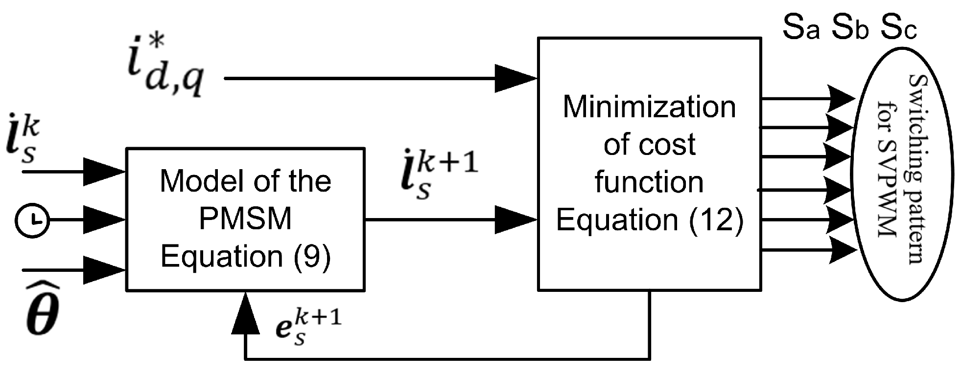
3.1. Modeling of Model Predictive Control

In this paper, the MPC is used due to multiple advantages, such as (a) MPC can equally handle both linear and nonlinear functions, (b) applicability on univariate and multivariate systems, (c) constraints handling and cost minimization, and (d) intuitive tuning parameters [30]. The discretized mathematical model of the PMSM in the $\mathit{dq}$-reference frame using the Taylor series for the MPC implementation is given as [26]:

$$\begin{array}{c}\hfill i_d^{k+1}=i_d^k-\left(\frac{R_s}{L_d}{i}_d^k+\frac{{\omega }_e{L}_q}{L_d}{i}_q^k+\frac{1}{L_d}{v}_d\right)T_s\end{array}$$

(8a)

$$\begin{array}{c}\hfill i_q^{k+1}=i_q^k-\left(\frac{{\omega }_e{L}_d}{L_q}{i}_d^k-\frac{R_s}{L_q}{i}_q^k+\frac{1}{L_q}{v}_q-\frac{{\omega }_e}{L_q}{\varphi }_f\right)T_s\end{array}$$

(8b)

The discretized model of the PMSM is summed up as state-space representation in Equation (9) which is used in the MPC block of Figure 1, where $i_d$ and $i_q$ currents are compared with reference currents. Three-phase currents are measured from the stator of the PMSM, converted into $\mathit{dq}$ transformation, and fed back to the MPC for comparison with the reference currents. All the parameters are constants in $A_{MPC}$ matrix except for the electrical speed ${\omega }_e$ which is increased or decreased as defined by the error vector of the objective function.

$$\begin{array}{c}\hfill {\mathbf{i}}_s^{k+1}=A_{MPC}{\mathbf{i}}_s^k+B_{MPC}{\mathbf{u}}_s\end{array}$$

(9)

where $A_{MPC}=\left[\begin{array}{cc}-\frac{R_s}{L_d}& \frac{{\omega }_e{L}_q}{L_d}\\ -\frac{{\omega }_e{L}_d}{L_q}& -\frac{R_s}{L_q}\end{array}\right]$, $B_{MPC}=\left[\begin{array}{cc}{L}_d& 0\\ 0& L_q\end{array}\right]$, and ${\mathbf{u}}_s=\left[\begin{array}{c}{v}_d\\ v_q-{\omega }_e{\varphi }_f\end{array}\right]$. The main objective is to compute the input vector for the MPC. For the modeling of the MPC algorithm, we initialize the current prediction value with ${\mathbf{i}}_{sm}^0=0$ for $k=0,1,2,3,\cdots ,\infty$. The iterative process will continue till the error reduces to the optimum level [11]. The predictive error vector is computed as:

$$\begin{array}{c}\hfill {\mathbf{e}}_s^{k+1}={\mathbf{i}}_s^{k+1}-{\mathbf{i}}_{sm}^{k+1|k}\end{array}$$

(10a)

$$\begin{array}{c}\hfill \left[\begin{array}{c}{\mathbf{i}}_{sp}^{k+1|k}\\ {\mathbf{i}}_{sp}^{k+2|k}\\ {\mathbf{i}}_{sp}^{k+3|k}\end{array}\right]=\left[\begin{array}{c}{\mathbf{i}}_{sm}^{k+1|k}\\ {\mathbf{i}}_{sm}^{k+2|k}\\ {\mathbf{i}}_{sm}^{k+3|k}\end{array}\right]+\mathbf{h}.{\mathbf{e}}_s^{k+1}\end{array}$$

(10b)

where $\mathbf{h}={\left[\begin{array}{ccc}{h}_1& h_2& h_3\end{array}\right]}^T$. Equation (10a) is the synchronous rotating frame stator current predictive error vector, which is calculated by the vector difference of current predictive values at time $k+1$ and k, respectively. According to the required reference speed, a correction factor h is used to correct the predictive values and the corrected current predictive value vector $i_{sp}$ is updated. Equation (10a) is used in Equation (10b) to update the predictive vector. The time-shifting is done by following equations in state-space while subscripts 0 shows the time-shifted vectors of the corrected predictive vector for the current values.

$$\begin{array}{c}\hfill \left[\begin{array}{c}{\mathbf{i}}_{s0}^{k+1|k}\\ {\mathbf{i}}_{s0}^{k+2|k}\\ {\mathbf{i}}_{s0}^{k+3|k}\end{array}\right]=\left[\begin{array}{ccc}0& 1& 0\\ 0& 0& 1\\ 0& 0& 1\end{array}\right]\left[\begin{array}{c}{\mathbf{i}}_{sp}^{k+1|k}\\ {\mathbf{i}}_{sp}^{k+2|k}\\ {\mathbf{i}}_{sp}^{k+3|k}\end{array}\right]\end{array}$$

(11)

Control inputs having incremental change $\Delta \mathbf{u}$ in stator voltage vector at time k and $k+1$ are defined within the constraints in the objective function as [29]:

$$\begin{array}{c}\hfill {\mathbf{u}}_s^{k+1}={\mathbf{u}}_s^k-\Delta {\mathbf{u}}_s^k\end{array}$$

(12)

where

$$\begin{array}{c}\hfill \Delta {\mathbf{u}}_s^k={\left({\mathbf{G}}_{MPC}^T{\mathbf{Q}}_{MPC}{\mathbf{G}}_{MPC}+{\mathbf{R}}_{MPC}\right)}^{-1}\\ \hfill {\mathbf{G}}_{MPC}^T{\mathbf{Q}}_{MPC}\left[\begin{array}{c}{\mathbf{i}}_s^{*k+1|k}-{\mathbf{i}}_{sp}^{k+1|k}\\ {\mathbf{i}}_s^{*k+2|k}-{\mathbf{i}}_{sp}^{k+2|k}\\ {\mathbf{i}}_s^{*k+3|k}-{\mathbf{i}}_{sp}^{k+3|k}\end{array}\right],\end{array}$$

$$\begin{array}{c}\hfill {\mathbf{Q}}_{MPC}=diag(q_1,q_2,q_3),\mathrm{and}{\mathbf{R}}_{MPC}=diag(r_1,r_2,r_3)\end{array}$$

All the components involved in $\Delta {\mathbf{u}}_s^k$ are defined in Table 2. In the final step, the current predictive value vector is updated using Equation (13).

$$\begin{array}{c}\hfill \left[\begin{array}{c}{\mathbf{i}}_{sm}^{k+1|k}\\ {\mathbf{i}}_{sm}^{k+2|k}\\ {\mathbf{i}}_{sm}^{k+3|k}\end{array}\right]=\left[\begin{array}{c}{\mathbf{i}}_{s0}^{k+1|k}\\ {\mathbf{i}}_{s0}^{k+1|k}\\ {\mathbf{i}}_{s0}^{k+1|k}\end{array}\right]+{\mathbf{G}}_{MPC}\left[\begin{array}{c}\Delta {\mathbf{u}}_s^k\\ \Delta {\mathbf{u}}_s^k\\ \Delta {\mathbf{u}}_s^k\end{array}\right]\end{array}$$

(13)

The process repeats until the error reduces to the minimum preset defined in the algorithm. Equation (12) is continuously being updated at each iteration, and then, this input is used in Equation (9). The switching state pattern is determined on the basis of error between reference currents and estimated currents. Using such a method, the MPC replaces the Field Oriented Control (FOC) technique previously used to determine switching state patterns for the PWM. Moreover, the MPC works in the feedforward mode to control the switching states of the IGBT that drives the PMSM. The block diagram of the MPC is illustrated in Figure 2.

3.2. Integrating SMO with MPC

This section presents the mathematical formulation of the SMO that is used in feedback mode to estimate the states of the system, as illustrated in Figure 1. There are two main stages of SMO, namely the sliding phase and the reachability phase. The stator voltages and currents are being utilized as inputs, and the SMO estimates the unknown Back EMF. The voltages are extracted from the switching states of the pulses as:

$$\begin{array}{c}\hfill \left[\begin{array}{c}{v}_a\\ v_b\\ v_c\end{array}\right]=\frac{v_{dc}}{3}\left[\begin{array}{ccc}2S_a& -S_b& -S_c\\ -S_a& 2S_b& -S_c\\ -S_a& -S_b& 2S_c\end{array}\right]\end{array}$$

(14)

A sliding surface is designed by the error difference equation between the estimated currents and measured currents to reach the sliding phase and the resulting error reduces to zero. A reaching phase control law is designed as follows [11]:

$$\begin{array}{c}\hfill u={\left[\begin{array}{cc}{K}_{sw}\mathrm{sgn}\left({\tilde{i}}_d\right)& K_{sw}\mathrm{sgn}\left({\tilde{i}}_q\right)\end{array}\right]}^T\end{array}$$

(15)

The signum function is used to reduce error when the sliding phase condition is met. The observer dynamics for currents are expressed as:

$$\begin{array}{c}\hfill \frac{d{\tilde{i}}_{dq}}{dt}=-\frac{R_s}{L_s}{\tilde{i}}_{dq}+\frac{1}{L_s}{v}_{dq}-\frac{K_{sw}}{L_s}\mathrm{sgn}\left({\tilde{i}}_{dq}\right)\end{array}$$

(16)

where ${\tilde{i}}_{dq}={\stackrel{⏜}{i}}_d-i_{dq}$. A positive definite Lyapunov candidate function is chosen as $V=\frac{1}{2}{S}^2$ and $K_{sw}=max\left(\left|v_d\right|,\left|v_q\right|\right)$ is derived as the reachability condition for the SMO. Both conditions are called Lyapunov asymptotic stability conditions. Currents obtained through Equation (16) are used as feedback reference currents for the MPC to compare with the measured currents.

3.3. Integrating EKF with MPC

The EKF, in reality, is an extension of a simple Kalman filter for nonlinear systems and works on the principle of the least square technique. It is based on successive linearization of the nonlinear state space model at each time instant around the previous estimate called Jacobian which is the linearized version of the nonlinear system. The Jacobians are calculated at each iteration using Equation (17a,b) [26].

$$\begin{array}{c}\hfill {\varphi }^k={\left.\frac{\partial f}{\partial x}\right|}_{x^k,u^k}\end{array}$$

(17a)

$$\begin{array}{c}\hfill {\mathbf{H}}^k={\left.\frac{\partial h}{\partial x}\right|}_{x^k}\end{array}$$

(17b)

Equation (17a) is the linearized version of the system matrix while Equation (17b) represents the linearized version for the output of the PMSM. Linearized function ${\varphi }^k$ and output function ${\mathbf{H}}^k$ of the nonlinear mathematical model are calculated. In the analysis of EKF, online computation of Jacobian matrices of both functions is necessary to predict the states and covariances [31]. Prediction and updating are the two major steps used for the estimation of the states. Integrating the EKF as an observer with the MPC, the following changes are to be made so that the simulation results can be compared with the proposed MPC-UKF scheme.

Step 1:

Prediction

$$\begin{array}{c}\hfill {\overline{\mathbf{x}}}^k=\mathbf{F}\left({\overline{\mathbf{x}}}^{k-1}\right){\overline{\mathbf{x}}}^{k-1}+\mathbf{B}{\mathbf{u}}^{k-1}\end{array}$$

(18a)

$$\begin{array}{c}\hfill {\mathbf{P}}^k={\varphi }^{k-1}{\mathbf{P}}^{k-1}{\left({\varphi }^{k-1}\right)}^T+{\mathbf{Q}}^k\end{array}$$

(18b)

Equation (18a) estimates the mean of next values for state-space vector ${\overline{\mathbf{x}}}^k$ in terms of the previous values of the states vector ${\overline{\mathbf{x}}}^{k-1}$ and the input vector ${\mathbf{u}}^{k-1}$ at instant $k-1$. The input vector is directly calculated from the stator voltages and converted into $dq$ transformation framework. Equation (18b) represents the estimation of covariance ${\mathbf{P}}^k$ in terms of Jacobian of the system matrix ${\varphi }^{k-1}$, initial assumption of covariance ${\mathbf{P}}^{k-1}$, and addition of process noise ${\mathbf{Q}}^k$ in the system.

Step 2:

Measurement

$$\begin{array}{c}\hfill {\overline{\mathbf{x}}}^k={\overline{\mathbf{x}}}^{k-1}+{\mathbf{K}}^k\left({\mathbf{y}}^k-\mathbf{H}{\overline{\mathbf{x}}}^{k-1}\right)\end{array}$$

(19a)

$$\begin{array}{c}\hfill {\mathbf{P}}^k={\mathbf{P}}^{k-1}-{\mathbf{K}}^k\mathbf{H}{\mathbf{P}}^k\end{array}$$

(19b)

$$\begin{array}{c}\hfill {\mathbf{K}}^k={\mathbf{P}}^{k-1}{\mathbf{H}}^T{\left(\mathbf{H}{\mathbf{P}}^{k-1}{\mathbf{H}}^T+{\mathbf{R}}^T\right)}^{-1}\end{array}$$

(19c)

$$\begin{array}{cc}\hfill {\mathbf{P}}^k& =\left(1-{\mathbf{K}}^k{\mathbf{H}}^{k-1}\right){\mathbf{P}}^{k-1}{(1-{\mathbf{K}}^k{\mathbf{H}}^{k-1})}^{-1}+\hfill \\ & {\mathbf{K}}^k{\mathbf{R}}^k{\left({\mathbf{K}}^k\right)}^T\hfill \end{array}$$

(19d)

Similarly, in the measurement phase, Equation (19a) updates the mean in stepwise process, such as (a) by measuring the direct, measurable states (stator currents) of the system that are in vector ${\mathbf{y}}^k$, (b) the term $\mathbf{H}{\overline{\mathbf{x}}}^{k-1}$ singles out the estimated states from the mean vector ${\overline{\mathbf{x}}}^{k-1}$, and (c) the difference between Equation (19a,b) is multiplied by Kalman Gain ${\mathbf{K}}^k$, which is calculated using Equation (19c). In Kalman gain, measurement noise ${\mathbf{R}}^T$ is added. Finally, Equation (19d) updates the covariance. This iterative process repeats itself until the specified number of iterations is achieved in the algorithm [3].

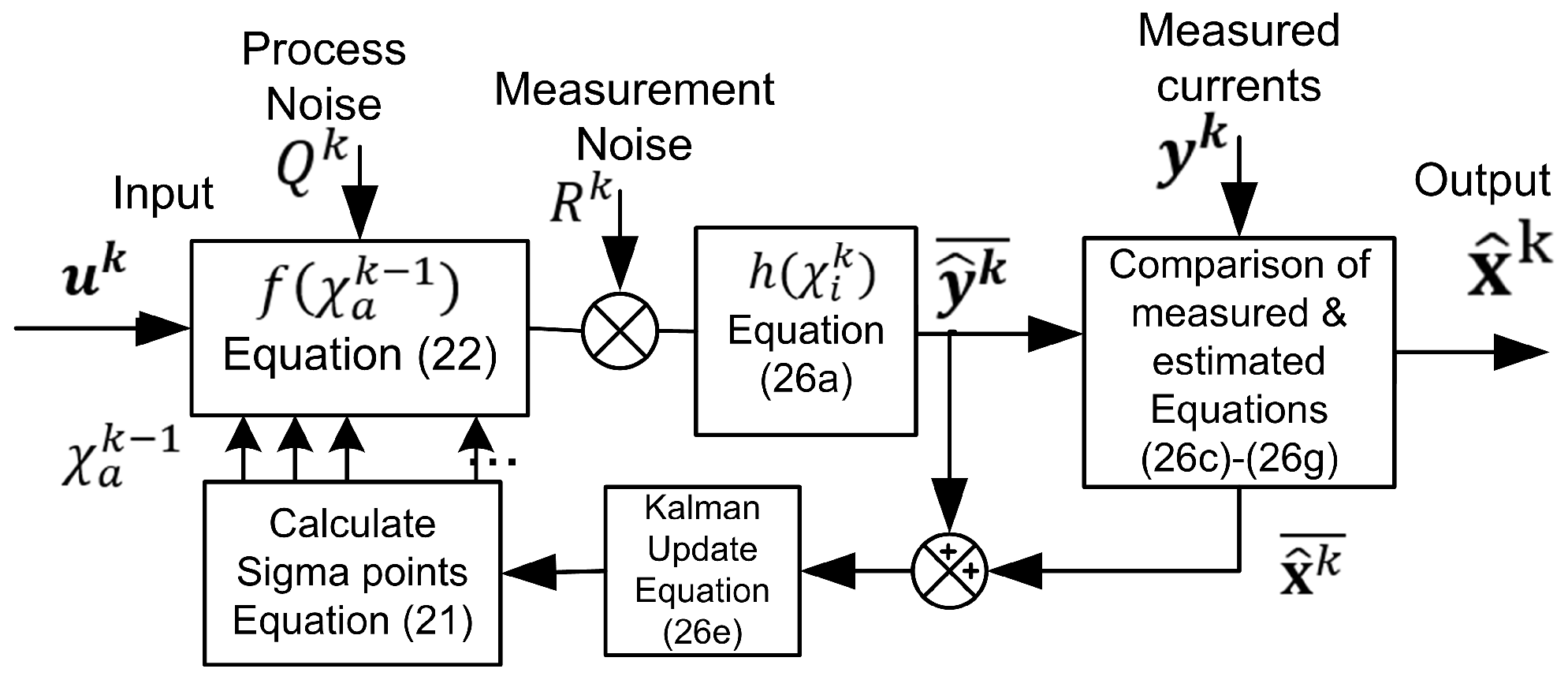
3.4. Integrating UKF with MPC

In this paper, we proposed a novel hybrid combination of UKF with MPC as a robust control algorithm for PMSM. The UKF algorithm consists of the following steps:

Step 1:

Initialization

$$\begin{array}{c}\hfill {\stackrel{⏜}{x}}_0=E\left[x_0\right]\end{array}$$

(20a)

Equation (20a) computes the mean (expected) values of the states. Initially, the mean states are chosen as zero vector. In the next iteration, sigma points generate nonzero states which are compared with the measured values. Similarly, the covariances are initialized in Equation (20b) at time instant 0.

$$\begin{array}{c}\hfill P_0=E\left[\left(x_0-{\stackrel{⏜}{x}}_0\right){\left(x_0-{\stackrel{⏜}{x}}_0\right)}^T\right]\end{array}$$

(20b)

Equation (20c) adds the process noise $E{\left(w^k\right)}^T$ and measurement noise $E{\left(v^k\right)}^T$ vectors in the estimation process to check the disturbance rejection of the UKF observer.

$$\begin{array}{c}\hfill {\stackrel{⏜}{x}}_0^a=E\left[x^a\right]={\left[\begin{array}{ccc}{\stackrel{⏜}{x}}_0^T& E{\left(w^k\right)}^T& E{\left(v^k\right)}^T\end{array}\right]}^T\end{array}$$

(20c)

Equation (20b) can be rewritten in matrix form as:

$$\begin{array}{c}\hfill P_0^a=E\left[\left(x_0^a-{\stackrel{⏜}{x}}_0^a\right){\left(x_0^a-{\stackrel{⏜}{x}}_0^a\right)}^T\right]=\left[\begin{array}{ccc}{P}_0& 0& 0\\ 0& Q^k& 0\\ 0& 0& R^k\end{array}\right]\end{array}$$

(20d)

where $Q^k=E\left(w{w}^T\right)$ and $R^k=E\left(v{v}^T\right)$ [29]. Equation (20d) is the calculation process of the successive covariances.

Step 2:

Calculation of Sigma Points

$$\begin{array}{c}\hfill {\chi }_0^{k-1}={\stackrel{⏜}{x}}^{k-1}\end{array}$$

(21a)

where ${\stackrel{⏜}{x}}^{k-1}$ is mean of a Gaussian. The mean value is initially set to a zero vector, and the value will be updated in every iteration. Sigma points are computed as follows [32]:

$$\begin{array}{c}\hfill {\chi }_i^{k-1}={\stackrel{⏜}{x}}^{k-1}+\sqrt{(n+\lambda )P_i^{k-1}}\end{array}$$

(21b)

$$\begin{array}{c}\hfill {\chi }_{i+1}^{k-1}={\stackrel{⏜}{x}}^{k-1}+\sqrt{(n+\lambda )P_i^{k-1}}\end{array}$$

(21c)

where $\lambda ={\alpha }^2(n+k)-n$ is a scaling parameter, and $\alpha$ value will be selected in the range of $1\le \alpha \le {10}^{-4}$, which determines the spread of sigma points around the mean value of the state vector. Equations (21b) and (21c) computes the upper and lower spread of sigma points to cover the estimated values, respectively.

$$\begin{array}{c}\hfill {\chi }_a^{k-1}=\left[\begin{array}{ccc}{\chi }_0^{k-1}& {\chi }_i^{k-1}& {\chi }_{i+1}^{k-1}\end{array}\right]\end{array}$$

(21d)

where the spread of sigma points is usually set to a small positive value, the constant $k=(3-n)$ is a secondary scaling parameter, and $\sqrt{(n+\lambda )P_i^{k-1}}$ is the ith column of the matrix square root (lower triangular Cholesky factorization) [32].

Step 3:

Propagation of Sigma Points through nonlinear function

The computed sigma points from step 2 are propagated through nonlinear function f, which is the mathematical model of PMSM given in Equation (4).

$$\begin{array}{c}\hfill {\chi }_i^k=f\left({\chi }_a^{k-1}\right),i=0,\cdots ,2n\end{array}$$

(22)

The mean and covariance for ${\chi }_i^k$ are approximated using a weighted sample mean, and covariance of the posterior sigma points, weights for mean and weights for covariance are calculated using Equations (23a,b) and (24a,b) respectively [33]:

$$\begin{array}{c}\hfill W_0^m=\frac{\lambda }{n+\lambda }\end{array}$$

(23a)

$$\begin{array}{c}\hfill W_i^m=\frac{1}{2(n+\lambda )},i=1,\cdots ,2n\end{array}$$

(23b)

$$\begin{array}{c}\hfill W_0^c=\frac{\lambda }{n+\lambda }+(1-{\alpha }^2+{\beta }^{\prime })\end{array}$$

(24a)

$$\begin{array}{c}\hfill W_i^c=W_i^m=\frac{1}{2(n+\lambda )},i=1,\cdots ,2n\end{array}$$

(24b)

In Equations (23) and (24), the subscripts m and c describe the weights for mean and covariance. The constant ${\beta }^{\prime }$ is the value of the distribution parameter whose optimal value is selected as 2 for a Gaussian distribution [33].

Step 4:

Prediction mean and covariance

Equation (25a) calculates the estimated mean of the states by averaging the sigma points through the multiplication of the weighted means. Similarly, Equation (25b) calculates the updated covariances by first computing the difference between estimated and measured values and then multiplying the resultant with the weighted covariance. Moreover, in step 4, the process noise $Q^k$ is added in the covariance matrix to check the disturbance rejection of the observer.

$$\begin{array}{c}\hfill \overline{{\stackrel{⏜}{x}}^k}=\sum _{i=0}^{2n}{W}_i^m{\stackrel{⏜}{\chi }}_i^k\end{array}$$

(25a)

$$\begin{array}{c}\hfill {\stackrel{⏜}{\mathbf{P}}}^k=\sum _{i=0}^{2n}{W}_i^c\left({\stackrel{⏜}{\chi }}_i^k-\overline{{\stackrel{⏜}{x}}^k}\right){\left({\stackrel{⏜}{\chi }}_i^k-\overline{{\stackrel{⏜}{x}}^k}\right)}^T+Q^k\end{array}$$

(25b)

Step 5:

Measurement update

Equation (26a) passes the sigma points through a function h that excludes the unobservable states, such as speed and angle from the observable states. In Equation (26a), the $Y_i^k$ is the vector output of the estimated speed and angle. The average of the vectors is calculated by multiplying Equation (26a) with the weighted mean, as shown in Equation (26b). Similarly, in Equation (26c,d), the covariances are estimated on the same pattern in the measurement step as calculated in the prediction step (step 4). However, the output vectors are utilized instead of the state vectors. Measurement noise $R^k$ is added in the measurement covariance matrix.

$$\begin{array}{c}\hfill Y_i^k=h\left({\chi }_i^k\right),i=1,\cdots ,2n\end{array}$$

(26a)

$$\begin{array}{c}\hfill \overline{{\stackrel{⏜}{y}}^k}=\sum _{i=0}^{2n}{W}_i^m{Y}_i^k\end{array}$$

(26b)

$$\begin{array}{c}\hfill {\mathbf{P}}_{yy}^k=\sum _{i=0}^{2n}{W}_i^c\left(Y_i^k-\overline{{\stackrel{⏜}{y}}^k}\right){\left(Y_i^k-\overline{{\stackrel{⏜}{y}}^k}\right)}^T+R^k\end{array}$$

(26c)

$$\begin{array}{c}\hfill {\mathbf{P}}_{xy}^k=\sum _{i=0}^{2n}{W}_i^c\left({\chi }_i^k-\overline{{\stackrel{⏜}{x}}^k}\right){\left(Y_i^k-\overline{{\stackrel{⏜}{y}}^k}\right)}^T\end{array}$$

(26d)

$$\begin{array}{c}\hfill {\mathbf{K}}^k={\mathbf{P}}_{xy}^k{\left({\mathbf{P}}_{yy}^k\right)}^{-1}\end{array}$$

(26e)

$$\begin{array}{c}\hfill {\stackrel{⏜}{\mathbf{x}}}^k=\overline{{\stackrel{⏜}{\mathbf{x}}}^k}+{\mathbf{K}}^k(y^k-\overline{{\stackrel{⏜}{y}}^k})\end{array}$$

(26f)

$$\begin{array}{c}\hfill {\mathbf{P}}^k={\overline{\mathbf{P}}}^k-\left({\mathbf{K}}^k\right){\mathbf{P}}_{yy}^k{\left({\mathbf{K}}^k\right)}^T\end{array}$$

(26g)

The iterative process of UKF is similar to the EKF algorithm until the optimized value is achieved except for the sigma point evaluation process. Equation (26e) estimates the Kalman gain while Equation (26f,g) calculate the estimated mean and covariance, respectively [34]. Equation (24f) is the final output of the UKF block in which two states, estimated speed, and angle, are extracted, and the speed is fed back to the PI controller, which proportionally converts it into reference current $i_q$ for the comparison with the measured current, as shown in Figure 1. The block diagram of UKF is illustrated in Figure 3.

4. Results and Discussions

To validate the performance of the proposed MPC-UKF technique, detailed simulation-based analysis and through comparisons are performed in MATLAB/Simulink. Every aspect of the simulation results is analyzed and visually obtained in graphs. Real-time PMSM parameters are selected for the PMSM system simulations to replicate the actual setup, as shown in

Table 3. Parameters Selected for PMSM System.

Symbol	Description	Value
${\varphi }_f$	amplitude of flux linkages	$7.8\times {10}^{-2}$ Wb $-t$
$B_{\omega }$	viscous friction coefficient	$3.023\times {10}^{-3}$ Nms/rad
$B_{\omega }$	col2 text	col3 text
$L_d$	direct axis inductance	$1.68\times {10}^{-2}$ H
$L_q$	quadrature axis inductance	$3.48\times {10}^{-2}$ H
$\rho$	number of poles	4
$R_s$	resistance of the stator	5 $\Omega$
$T_s$	sampling time	$2\times {10}^{-4}$ s
J	moment of inertia	$2.3\times {10}^{-5}$ kg cm2

.

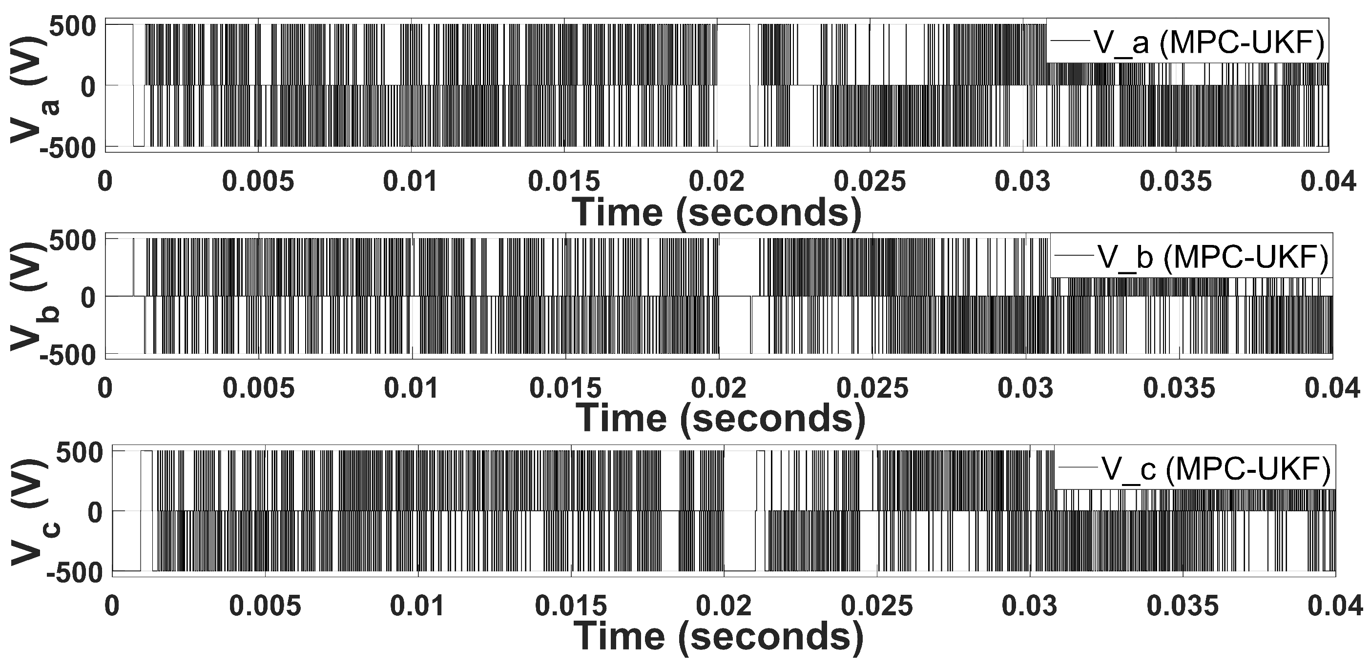
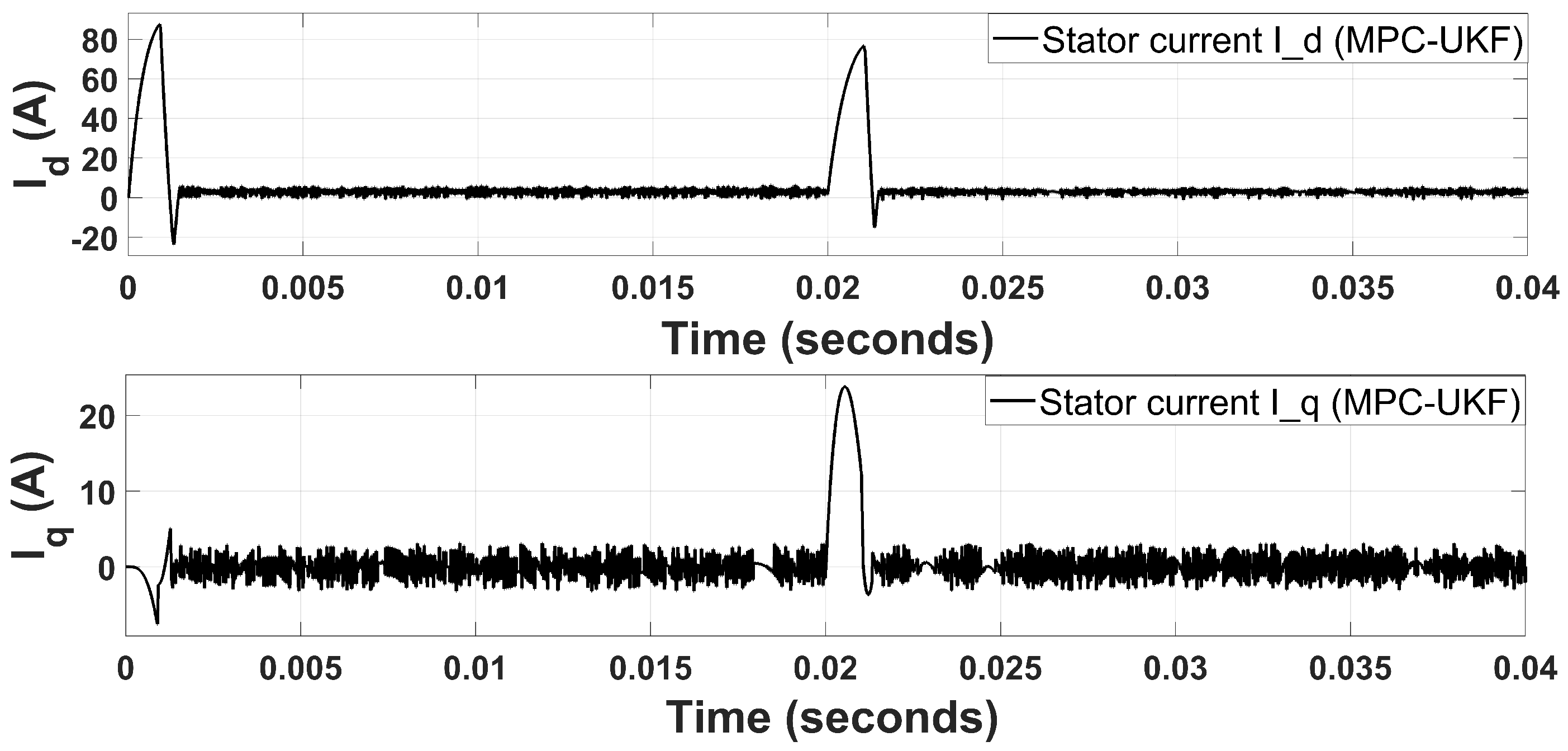
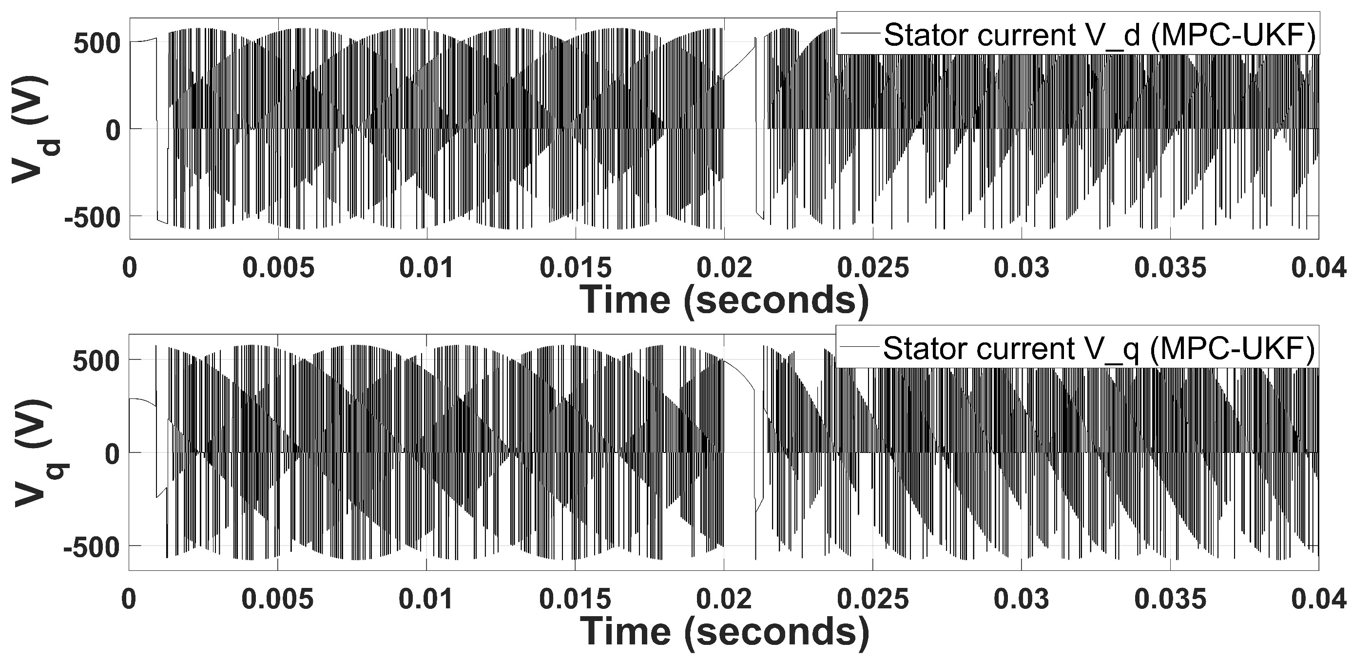
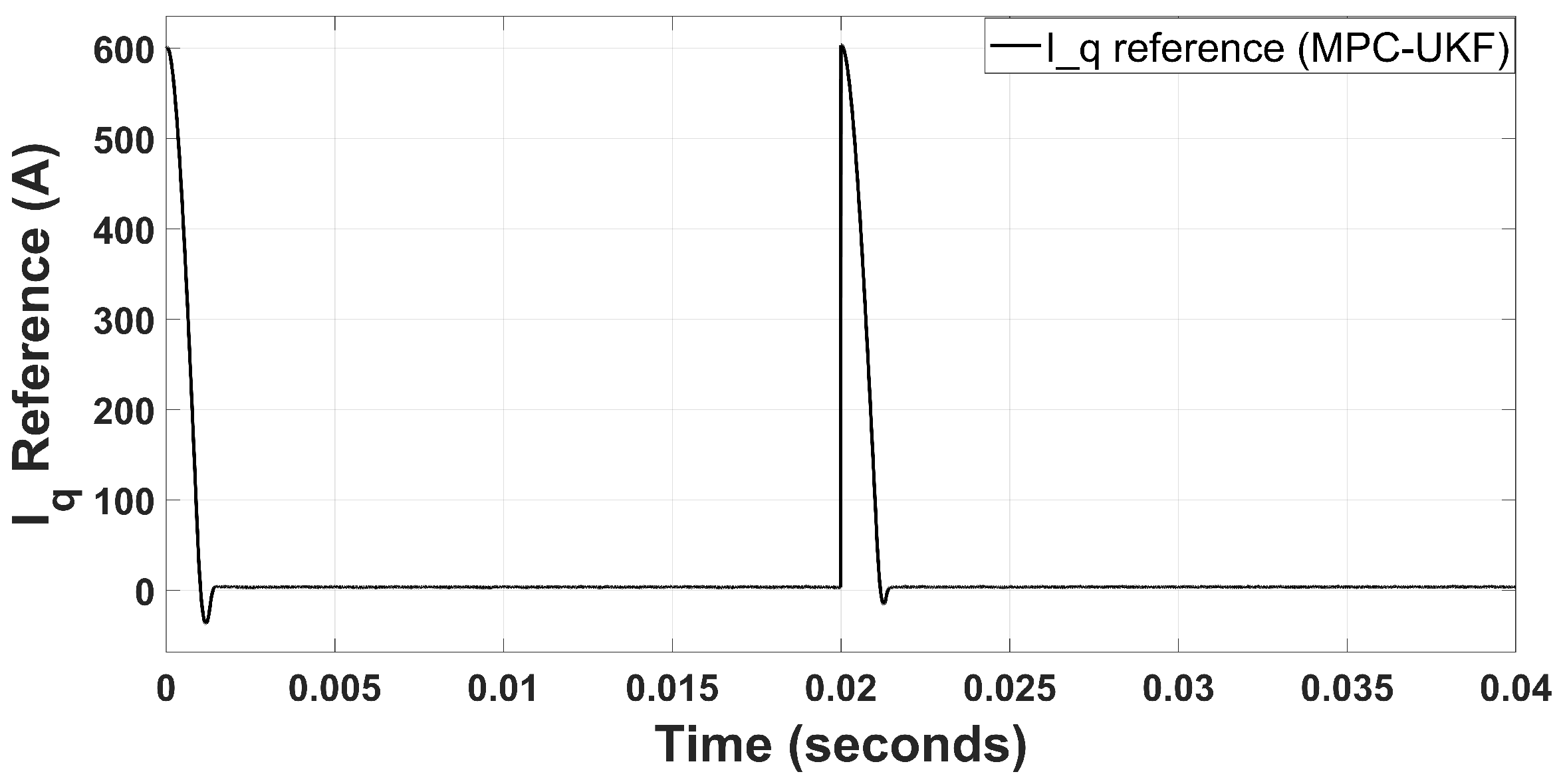
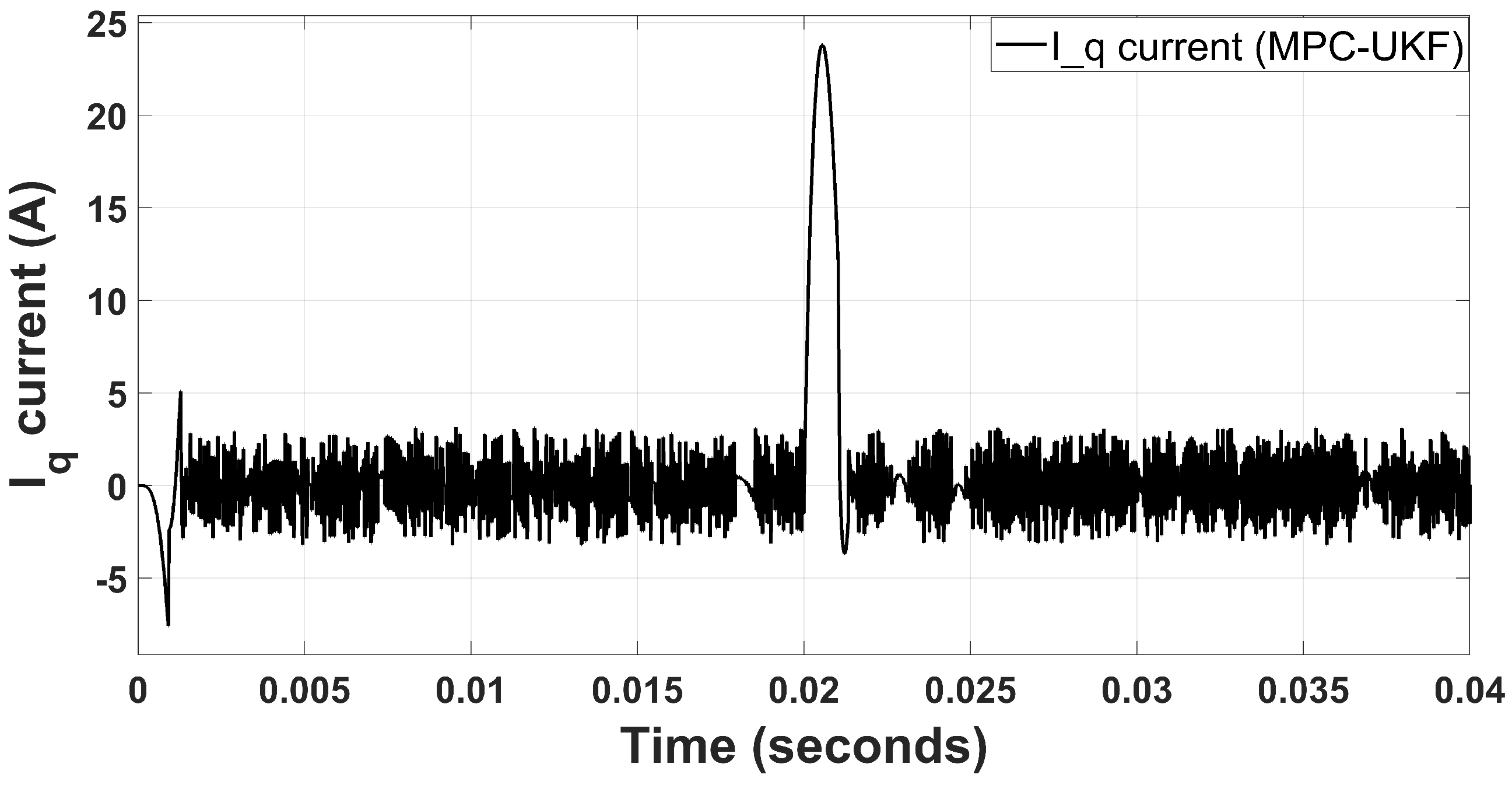
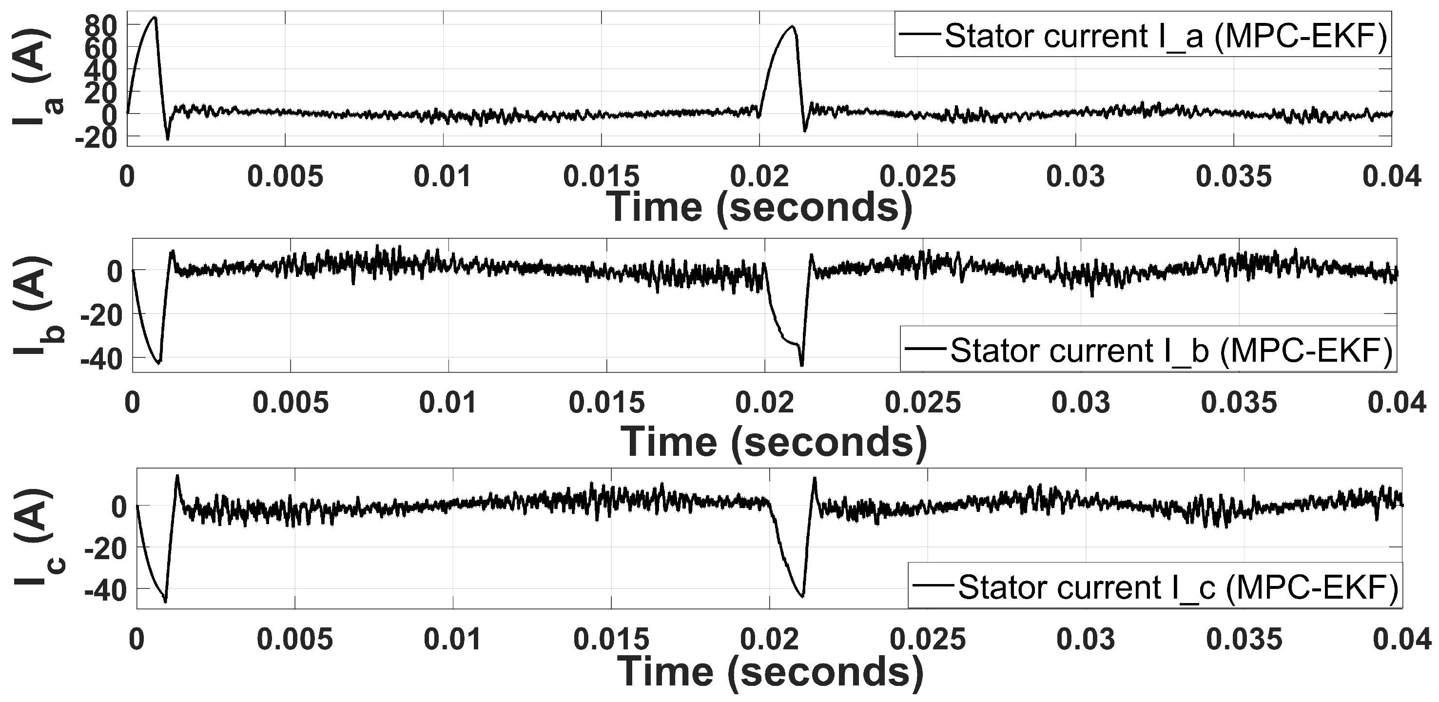
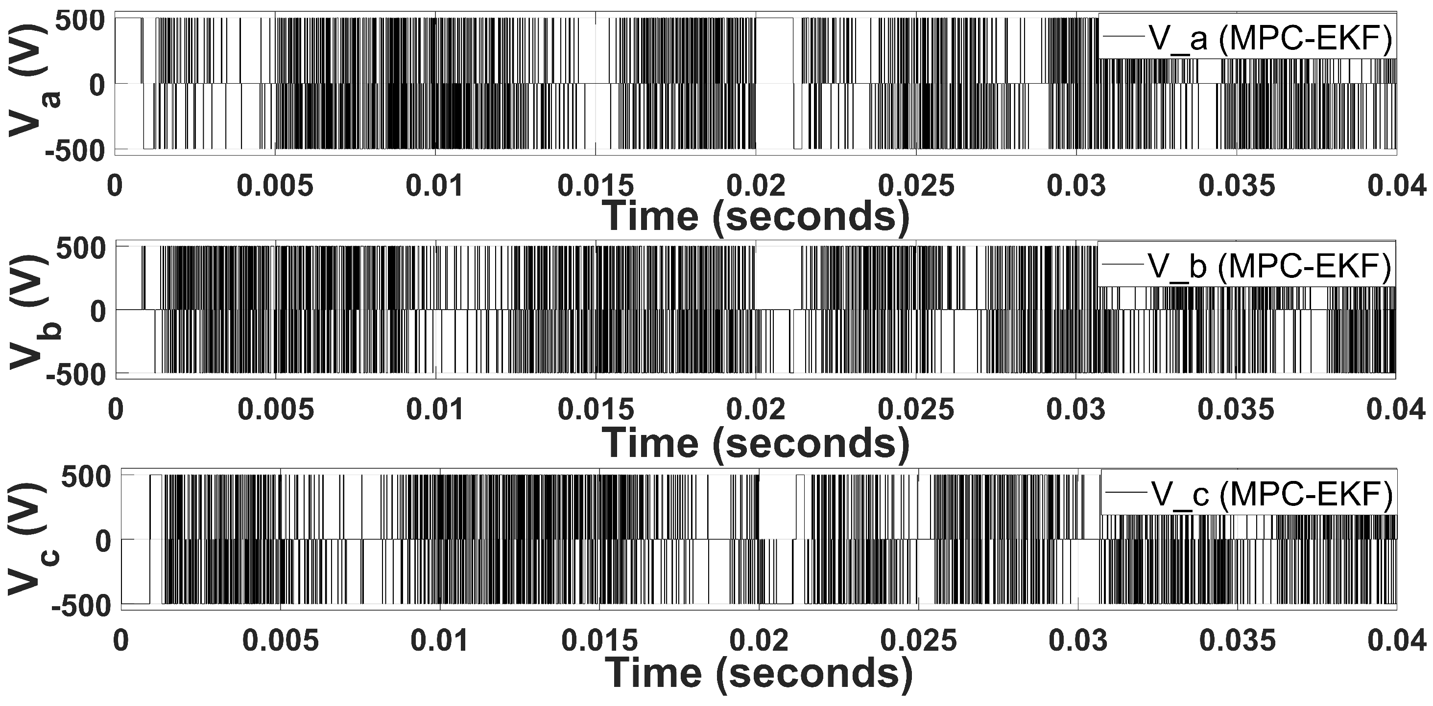
4.1. Stator Current and Voltage Comparison

The three-phase stator currents of the PMSM are plotted in Figure 4, the current spike in the start shows the inherent nature of the motor’s inrush current. However, the current stabilizes in less than 1 millisecond. A second spike occurs when the speed changes from 300 rad/s to 600 rad/s. The second spike is less aggressive because high-speed performance is more accurate compared to starting/low speed performance. Ripples in stator current waveforms are not so deviating due to the accurate prediction behavior of the UKF. Similarly, the three-phase voltages of the PMSM are plotted in Figure 5. Similar behavior is observed in three-phase voltages as observed in three-phase stator currents. The switching states signal of the inverter’s IGBTs are generated by the MPC, as shown in Figure 5. When the PWM signals are concentrated, it represents very low duty cycle that is adjusted based on harmonics and disturbances involved in the system. When process noise or measurement noise is low, the duty cycle considerably increases. The state space vectors controlled by the MPC generate the currents and voltages shown in Figure 4 and Figure 5, respectively. Park’s transformation is used to convert three-phase $\mathit{abc}$ to $\mathit{dq}$ axis coordinates, and the resultant plots of currents and voltages are shown in Figure 6 and Figure 7, respectively. The back EMF generated by the PMSM is sinusoidal; therefore, after conversion from three-phase $\mathit{abc}$ to $\mathit{dq}$, switching states of the PWM are converted to sinusoidal waveforms. Moreover, the currents after transformation remain the same. Current peaks are the same in $\mathit{dq}$ coordinates as they are in three-phase coordinates. The MPC-UKF shows promising results because of less ripples in currents and voltages.

Stator voltages are sinusoidal because the PMSM has sinusoidal back EMF. Stator voltages are stable and do not have peak values because VSI converts from current switching states to voltage switching states to be measured and used for the estimation of the states (speed/position) directly using UKF algorithm. In Figure 1, the error between the predicted speed from UKF observer and reference speed acts as an input for the PI controller, and the PI controller generates a proportional current for the MPC so that the states can be generated according to the difference between the reference speed and the estimated speed. It is represented in Figure 8 that the reference current generated by the PI controller is very smooth except at the starting and where the input reference step changes. In Figure 8, the peaks are generated to counter the effect of inrush current behavior.

Similarly, Figure 9 shows the measured current after $\mathit{dq}$ transformation, and this current is compared with the reference current for the PI controller. The difference of both currents determines the frequency of switching states accordingly. The proposed hybrid MPC-UKF scheme is more robust for parametric variation and noise. However, an overshoot is observed due to aggressive achievement of steady-state. The receding horizon in the MPC is chosen as one step because the feedback-estimated values through the UKF constantly determine the change in the input for the MPC. Finally, the MPC predicts the constant values from the observer (UKF) when the reference values become constant. In the steady-state, no ripples arise since the UKF rejects the noise and is resilient to parametric invariance. Therefore, a steady state level can be achieved by the advantages of the UKF.

For comparative analysis, every aspect of the simulation results is analyzed and visualized graphically compared to MPC-EKF and MPC-SMO. For MPC-EKF, three-phase motor currents are obtained and plotted in Figure 10. In Figure 10, the ripples in stator current waveforms are abrupt due to the linearization-based behavior of the system matrix, which is called Jacobian of the EKF algorithm. Similarly, Figure 11 illustrates the observed voltage vectors for MPC-EKF. In the MPC-EKF, combination performance degrades because the EKF cannot tackle nonlinearities efficiently. Therefore, where the noise/disturbance level increases, variation in voltage also increases, as shown in Figure 11. Similar distorted behavior is observed in the stator current and voltage in the $\mathit{dq}$-framework because the EKF is a linearization approach. Therefore, the estimation of states is not accurate, and noise prevails in the system.

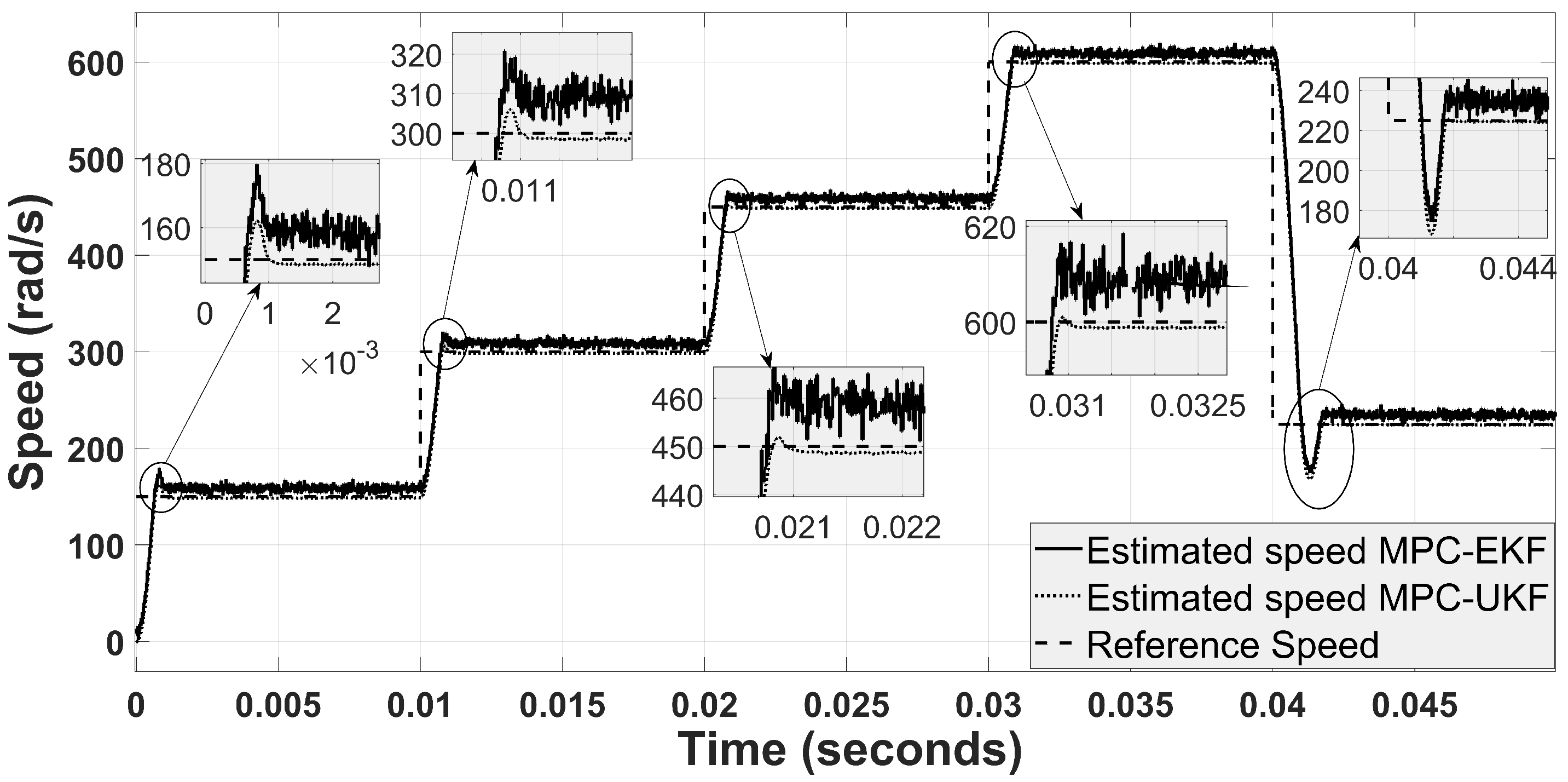
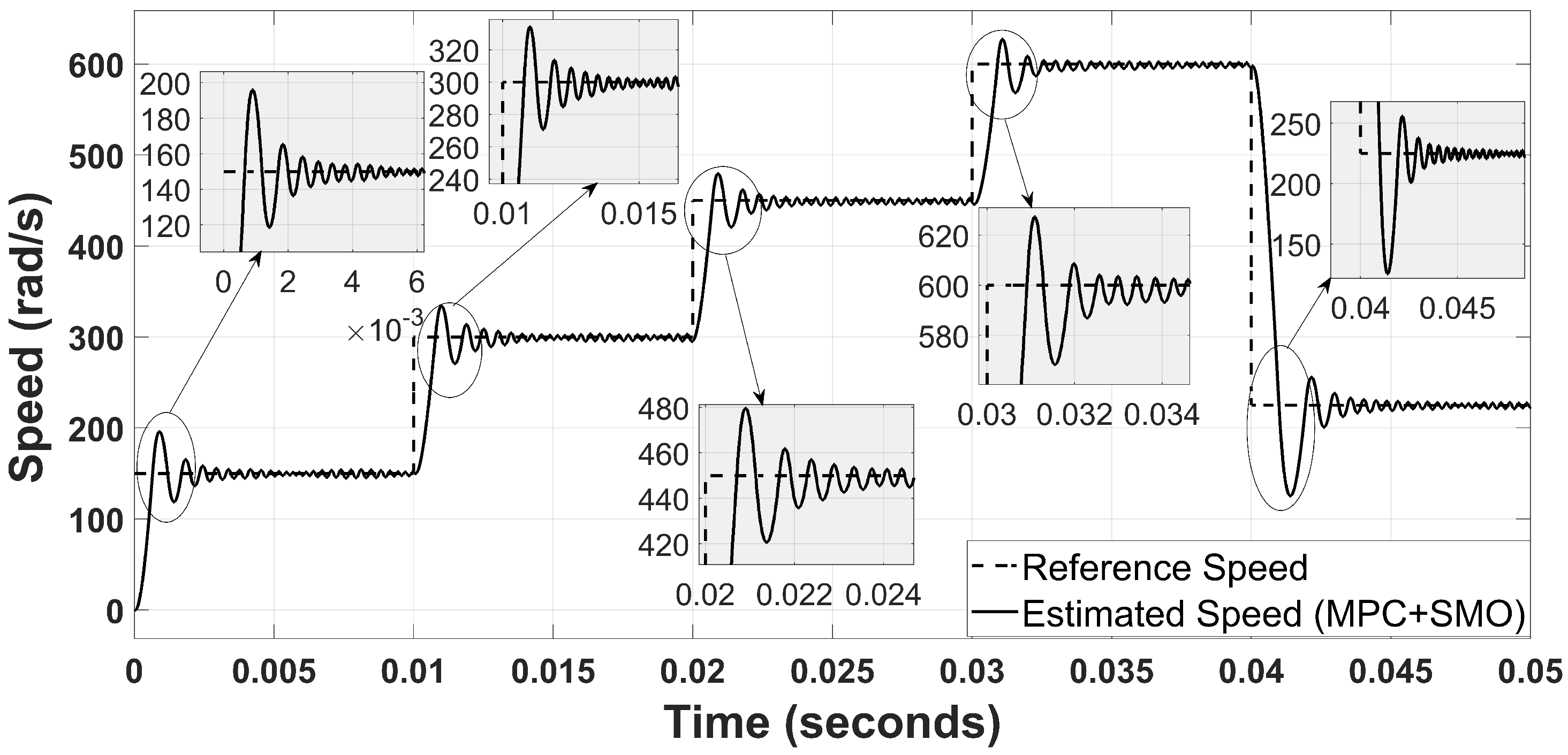
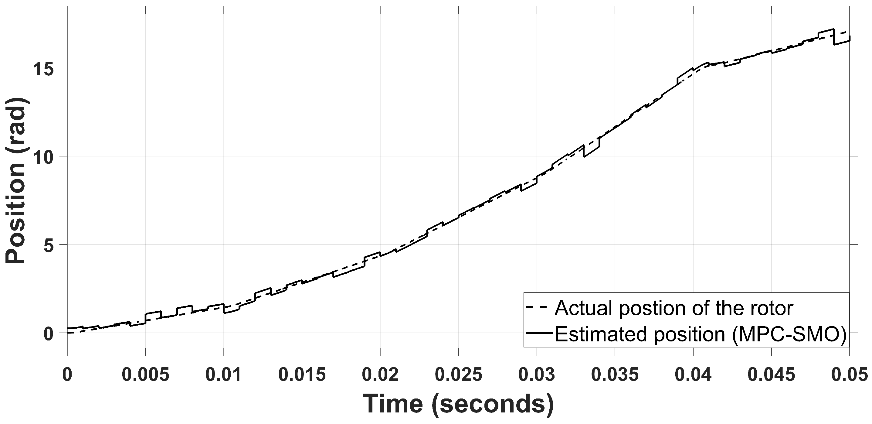
4.2. Speed and Position Comparison

To further elaborate the performance of the proposed hybrid MPC-UKF technique, we compare the estimation of speed and position under multiple-step change in the reference values. To check the robustness, five-speed references are imposed, such as 150 rad/s, 300 rad/s, 450 rad/s, 600 rad/s, and 225 rad/s. The comparative analysis of speed estimation under the control algorithm of MPC-UKF and MPC-EKF is shown in Figure 12. The graph in Figure 12 shows the accuracy of MPC-UKF as PWM manipulation is better compared to MPC-EKF. In Figure 12, the MPC with the EKF achieves a steady state speed in less than 1.5 milliseconds; however, the ripples remain constant during the whole step. Moreover, an overshoot is observed for every reference speed change due to aggressive achievement of steady-state, and ripples also propagate in the steady-state behavior because of the highly nonlinear system of the PMSM. The EKF could not handle the highly nonlinear systems since it approximates the mathematical model of the PMSM up to 1st order by using a Taylor series expansion. However, no overshoot and ripples are observed for MPC-UKF. Therefore, in MPC-EKF, speed estimation is not accurate compared to MPC-UKF. Moreover, the parametric invariance of the EKF is not robust enough to remove the harmonics or internal disturbances. Furthermore, the receding horizon in the MPC is chosen as one step ahead because the feedback-estimated values through the UKF or EKF constantly determine the change in the input for the MPC. The MPC predicts the constant values from the observer when the reference value becomes steady. In the steady-state, ripples arise since the EKF could not reject the noise and is resilient to parametric invariance.

Another combination is analyzed by replacing the EKF with the SMO, and results are depicted in Figure 13. For MPC-SMO, the estimation is not stable due to the chattering effect of the SMO. Moreover, the percentage overshoot and settling time are greater compared to MPC-UKF and MPC-EKF. However, the noise level/ripples are negligible compared to MPC-EKF, while comparative to MPC-UKF. Therefore, MPC-SMO is very robust to parametric variation. A similar observation is noted for position estimation. The graphical comparison of MPC-UKF with MPC-EKF and MPC-SMO is illustrated in Figure 14 and Figure 15.

A detailed quantitative analysis of the proposed MPC-UKF technique with MPC-EKF and MPC-SMO is presented in

Table 4. PMSM parameters used in the Simulations.

Dynamic Property	MPC-UKF	MPC-EKF	MPC-SMO	Percentage Improvement for UKF
Step 1 (0–25% of rated speed)
Speed peak time	0.75 ms	1.07 ms	1.59 ms	29.90%
Speed settling time	0.97 ms	1.15 ms	3.50 ms	15.65%
Speed overshoot	1.26%	1.78%	24.9%	29.21%
Step 2 (25–50% of rated speed)
Speed peak time	0.68 ms	1 ms	1.48 ms	32%
Speed settling time	0.67 ms	0.87 ms	3.06 ms	22.98%
Speed overshoot	0.92%	1.43%	19.6%	35.66%
Step 3 (50–75% of rated speed)
Speed peak time	0.65 ms	0.91 ms	2.05 ms	28.57%
Speed settling time	0.34 ms	0.52 ms	2.59 ms	34.61%
Speed overshoot	0.56%	0.99%	15.4%	43.43%
Step 4 (75–100% of rated speed)
Speed peak time	0.42 ms	0.61 ms	2.60 ms	31.14%
Speed settling time	0.26 ms	0.35 ms	2.36 ms	25.71%
Speed overshoot	0.29%	0.78%	11.56%	62.82%
Step 5 (40% of rated speed)
Speed peak time	1.21 ms	1.36 ms	4.89 ms	11.03%
Speed settling time	0.97 ms	1.15 ms	3.50 ms	15.65%
Speed overshoot	1.26%	1.78%	24.9%	29.21%

. The results clearly indicate that MPC-UKF outperforms the other two techniques. Therefore, it is evident that the MPC with UKF produces smoother and more accurate results as EKF linearizes the system model and therefore develops inaccuracy. After the transient period, steady-state error in MPC-UKF reduces to zero while the error persists in MPC-EKF. The complexity level of MPC-UKF and MPC-EKF is almost similar, but under noisy conditions; MPC-UKF is more promising for highly nonlinear and complex systems, and it is robust and indifferent to parametric variation. However, the execution time of the MPC-UKF is higher compared to MPC-EKF and MPC-SMO because the UKF must compute sigma points at each sampling interval.

5. Conclusions and Future Work

The highly nonlinear behavior, rapidly varying dynamics, and practically unavailable measurements make PMSM a challenging estimation and control problem. In order to cope with such challenges, a novel hybrid strategy of MPC-UKF is proposed that provides advantages over the previously used algorithms in the shape of fewer current ripples, short peak time, improved settling time, controlled overshoot regarding speed variations, and an overall improved estimation. Therefore, the MPC-UKF hybrid approach, as a whole, is less susceptible to speed variations. In an effort to present an insightful discussion, the MPC-UKF has been compared with the MPC-EKF and MPC-SMO and it has been shown that the MPC-UKF has a good dynamic response even in a wide range with safer starting procedures. The superiority of the MPC-UKF over the other two approaches particularly originates from the fact that the UKF copes with the high nonlinearities, uncertainties, and unobservability more efficiently as compared to the EKF and SMO. It can be concluded from the presented results that the combination of MPC and the UKF is comparatively an efficient and better choice for high-performance AC drives. The proposed method seems amenable to highly nonlinear AC drives based on Doubly Fed Induction Motor (DFIM) and would potentially prove advantageous. In the future, we will intend to validate the proposed hybrid MPC-UKF technique through practical experimentation [35,36]. Moreover, state-of-the-art observers, such as the improved non-singular fast terminal SMC and second-order SMC, will be implemented and compared in a hybrid combination with MPC.

References

1. Ali, S.M.; Jawad, M.; Guo, F.; Mehmood, A.; Khan, B.; Glower, J.; Khan, S.U. Exact feedback linearization-based permanent magnet synchronous generator control. Int. Trans. Electr. Energy Syst. 2016, 26, 1917–1939. [Google Scholar] [CrossRef]
2. Blazek, V.; Slanina, Z.; Petruzela, M.; Hrbáč, R.; Vysockỳ, J.; Prokop, L.; Misak, S.; Walendziuk, W. Error Analysis of Narrowband Power-Line Communication in the Off-Grid Electrical System. Sensors 2022, 22, 2265. [Google Scholar] [CrossRef]
3. Yin, Z.; Li, G.; Zhang, Y.; Liu, J.; Sun, X.; Zhong, Y. A speed and flux observer of induction motor based on extended Kalman filter and Markov chain. IEEE Trans. Power Electron. 2016, 32, 7096–7117. [Google Scholar] [CrossRef]
4. Mehmood, C.A.; Nasim, R.; Ali, S.M.; Jawad, M.; Usman, S.; Khan, S.; Salahuddin, S.; Ihsan, M.A.; Khawja, A. Robust speed control of interior permanent magnet synchronous machine “fractional order control”. In Proceedings of the IEEE International Conference on Electro/Information Technology, Milwaukee, WI, USA, 5–7 June 2014; IEEE: Piscataway, NJ, USA, 2014; pp. 197–201. [Google Scholar]
5. Xu, D.; Wang, B.; Zhang, G.; Wang, G.; Yu, Y. A review of sensorless control methods for AC motor drives. CES Trans. Electr. Mach. Syst. 2018, 2, 104–115. [Google Scholar] [CrossRef]
6. Wang, F.; Mei, X.; Rodriguez, J.; Kennel, R. Model predictive control for electrical drive systems—An overview. CES Trans. Electr. Mach. Syst. 2017, 1, 219–230. [Google Scholar] [CrossRef]
7. Borsje, P.; Chan, T.; Wong, Y.; Ho, S.L. A comparative study of Kalman filtering for sensorless control of a permanent-magnet synchronous motor drive. In Proceedings of the IEEE International Conference on Electric Machines and Drives, San Antonio, TX, USA, 15 May 2005; IEEE: Piscataway, NJ, USA, 2005; pp. 815–822. [Google Scholar]
8. Yin, Z.; Li, G.; Du, C.; Sun, X.; Liu, J.; Zhong, Y. An adaptive speed estimation method based on a strong tracking extended Kalman filter with a least-square algorithm for induction motors. J. Power Electron. 2017, 17, 149–160. [Google Scholar] [CrossRef]
9. Madhukar, P.S.; Prasad, L. State Estimation using Extended Kalman Filter and Unscented Kalman Filter. In Proceedings of the 2020 International Conference on Emerging Trends in Communication, Control and Computing (ICONC3), Lakshmangarh, India, 21–22 February 2020; IEEE: Piscataway, NJ, USA, 2020; pp. 1–4. [Google Scholar]
10. Zerdali, E. Adaptive extended Kalman filter for speed-sensorless control of induction motors. IEEE Trans. Energy Convers. 2018, 34, 789–800. [Google Scholar] [CrossRef]
11. Wang, Y.; Zhang, Z.; Huang, W.; Kennel, R.; Xie, W.; Wang, F. Encoderless sequential predictive torque control with SMO of 3L-NPC converter-fed induction motor drives for electrical car applications. In Proceedings of the 2019 IEEE International Symposium on Predictive Control of Electrical Drives and Power Electronics (PRECEDE), Quanzhou, China, 31 May–2 June 2019; IEEE: Piscataway, NJ, USA, 2019; pp. 1–6. [Google Scholar]
12. Zerdali, E.; Barut, M. The comparisons of optimized extended Kalman filters for speed-sensorless control of induction motors. IEEE Trans. Ind. Electron. 2017, 64, 4340–4351. [Google Scholar] [CrossRef]
13. Karamanakos, P.; Geyer, T.; Kennel, R. On the choice of norm in finite control set model predictive control. IEEE Trans. Power Electron. 2017, 33, 7105–7117. [Google Scholar] [CrossRef]
14. Abokhalil, A. Rotor Position Estimation of PMSM for Low and High Rotor Speed. J. Eng. Res. 2021, 9, 161–170. [Google Scholar]
15. Haykin, S. Kalman Filtering and Neural Networks; John Wiley & Sons: Hoboken, NJ, USA, 2004; Volume 47. [Google Scholar]
16. Duan, Z.; Akhtar, J.; Ghous, I.; Jawad, M.; Khosa, I.; Ali, K. Improving the tracking of subatomic particles using the unscented Kalman filter with measurement redundancy in high energy physics experiments. IEEE Access 2019, 7, 61728–61737. [Google Scholar] [CrossRef]
17. Wang, F.; Davari, S.A.; Chen, Z.; Zhang, Z.; Khaburi, D.A.; Rodríguez, J.; Kennel, R. Finite control set model predictive torque control of induction machine with a robust adaptive observer. IEEE Trans. Ind. Electron. 2016, 64, 2631–2641. [Google Scholar] [CrossRef]
18. Szabat, K.; Wróbel, K.; Dróżdż, K.; Janiszewski, D.; Pajchrowski, T.; Wójcik, A. A fuzzy unscented Kalman filter in the adaptive control system of a drive system with a flexible joint. Energies 2020, 13, 2056. [Google Scholar] [CrossRef]
19. Wang, W.; Lu, Z.; Hua, W.; Wang, Z.; Cheng, M. A Hybrid Dual-Mode Control for Permanent-Magnet Synchronous Motor Drives. IEEE Access 2020, 8, 105864–105873. [Google Scholar] [CrossRef]
20. Zawirski, K.; Janiszewski, D.; Muszynski, R. Unscented and extended Kalman filters study for sensorless control of PM synchronous motors with load torque estimation. Bull. Pol. Acad. Sci. Tech. Sci. 2013, 61, 793–801. [Google Scholar] [CrossRef]
21. Zhang, X.; Zhao, Z. Multi-stage Series Model Predictive Control for PMSM Drives. IEEE Trans. Veh. Technol. 2021, 70, 6591–6600. [Google Scholar] [CrossRef]
22. Jafarzadeh, S.; Lascu, C.; Fadali, M.S. State estimation of induction motor drives using the unscented Kalman filter. IEEE Trans. Ind. Electron. 2011, 59, 4207–4216. [Google Scholar] [CrossRef]
23. Li, J.; Zhang, L.H.; Niu, Y.; Ren, H.P. Model predictive control for extended Kalman filter based speed sensorless induction motor drives. In Proceedings of the 2016 IEEE Applied Power Electronics Conference and Exposition (APEC), Long Beach, CA, USA, 20–24 March 2016; IEEE: Piscataway, NJ, USA, 2016; pp. 2770–2775. [Google Scholar]
24. Zhang, X.; Zhao, Z. Model Predictive Control for PMSM Drives with Variable Dead-Zone Time. IEEE Trans. Power Electron. 2021, 36, 10514–10525. [Google Scholar] [CrossRef]
25. Maanani, Y.; Menacer, A.; Harzelli, I. Comparative Study Between Sensorless Vector Control and Nonlinear Control for PMSM Based on Extended Kalman Filter (EKF). In Proceedings of the International Conference on Engineering Technologies (ICENTE’17), Konya, Turkey, 20–24 December 2017; pp. 173–185. [Google Scholar]
26. Martin, C.; Arahal, M.R.; Barrero, F.; Durán, M.J. Five-phase induction motor rotor current observer for finite control set model predictive control of stator current. IEEE Trans. Ind. Electron. 2016, 63, 4527–4538. [Google Scholar] [CrossRef]
27. Toso, F.; Da Ru, D.; Alotto, P.; Bolognani, S. A moving horizon estimator for the speed and rotor position of a sensorless pmsm drive. IEEE Trans. Power Electron. 2018, 34, 580–587. [Google Scholar] [CrossRef]
28. Wei, Y.; Wei, Y.; Gao, Y.; Qi, H.; Guo, X.; Li, M.; Zhang, D. A Variable Prediction Horizon Self-tuning Method for Nonlinear Model Predictive Speed Control on PMSM Rotor Position System. IEEE Access 2021, 9, 78812–78822. [Google Scholar] [CrossRef]
29. Yang, C.; Shi, W.; Chen, W. Comparison of unscented and extended Kalman filters with application in vehicle navigation. J. Navig. 2017, 70, 411–431. [Google Scholar] [CrossRef]
30. Guzman, H.; Duran, M.J.; Barrero, F.; Zarri, L.; Bogado, B.; Prieto, I.G.; Arahal, M.R. Comparative study of predictive and resonant controllers in fault-tolerant five-phase induction motor drives. IEEE Trans. Ind. Electron. 2015, 63, 606–617. [Google Scholar] [CrossRef]
31. Moon, C.; Kwon, Y.A. Sensorless speed control of a permanent magnet synchronous motor using an unscented Kalman filter with compensated covariances. J. Adv. Mar. Eng. Technol. 2020, 44, 42–47. [Google Scholar] [CrossRef]
32. Lešić, V.; Vašak, M.; Stojičić, G.; Perić, N.; Joksimović, G.; Wolbank, T.M. State and parameter estimation for field-oriented control of induction machine based on unscented Kalman filter. In Proceedings of the International Symposium on Power Electronics Power Electronics, Electrical Drives, Automation and Motion, Sorrento, Italy, 20–22 June 2012; IEEE: Piscataway, NJ, USA, 2012; pp. 409–414. [Google Scholar]
33. Sel, A.; Sel, B.; Kasnakoglu, C. GLSDC Based Parameter Estimation Algorithm for a PMSM Model. Energies 2021, 14, 611. [Google Scholar] [CrossRef]
34. Xu, B.; Mu, F.; Shi, G.; Ji, W.; Zhu, H. State estimation of permanent magnet synchronous motor using improved square root UKF. Energies 2016, 9, 489. [Google Scholar] [CrossRef]
35. Xu, B.; Zhang, L.; Ji, W. Improved non-singular fast terminal sliding mode control with disturbance observer for PMSM drives. IEEE Trans. Transp. Electrif. 2021, 7, 2753–2762. [Google Scholar] [CrossRef]
36. Liu, L.; Ding, S.; Yu, X. Second-order sliding mode control design subject to an asymmetric output constraint. IEEE Trans. Circuits Syst. II Express Briefs 2020, 68, 1278–1282. [Google Scholar] [CrossRef]
Figure 1. Schematic diagram of the proposed scheme.
Applsci 12 04958 g001
Figure 2. Finite Control Set-Model Predictive Control (FCS-MPC) internal modeling.
Applsci 12 04958 g002
Figure 3. UKF nonlinear modeling for PMSM.
Applsci 12 04958 g003
Figure 4. Three-phase stator currents for MPC-UKF.
Applsci 12 04958 g004
Figure 5. Three-phase stator voltages for MPC-UKF.
Applsci 12 04958 g005
Figure 6. dq -reference stator currents for MPC-UKF.
Applsci 12 04958 g006
Figure 7. dq -reference stator voltages for MPC-UKF.
Applsci 12 04958 g007
Figure 8. Reference current for MPC-UKF.
Applsci 12 04958 g008
Figure 9. Feedback current for MPC-UKF.
Applsci 12 04958 g009
Figure 10. Three-phase stator currents for MPC-EKF.
Applsci 12 04958 g010
Figure 11. Three-phase stator voltages for MPC-EKF.
Applsci 12 04958 g011
Figure 12. Speed estimation comparison of MPC-UKF and MPC-EKF.
Applsci 12 04958 g012
Figure 13. Speed estimation with MPC-SMO.
Applsci 12 04958 g013
Figure 14. Position estimation comparison for MPC-UKF and MPC-EKF.
Applsci 12 04958 g014
Figure 15. Position estimation with MPC-SMO.
Applsci 12 04958 g015