Gaussian Processes for Signal Processing and Representation in Control Engineering

Abstract

The Gaussian process is an increasingly well-known type of stochastic process, which is a generalization of the Gaussian probability distribution. It allows us to model complex functions thanks to its flexibility, which would not be possible with the use of other tools. Gaussian processes also have a couple of other features that are used in various branches of automation with positive results, ranging from industrial processes to image processing. There are also many ways of setting up the Gaussian processes, which required knowledge on the topic and depend on the presented problem. Considerations on these topics lead to the conclusion that the current state of practical usefulness of Gaussian processes increases significantly, therefore the deepening of knowledge about the ways of its use is highly suggested. In this review, we present selected technical applications of Gaussian Processes allowing an understanding of their broad applicability.

1. Introduction

Complicated phenomena surround us, motivating us to find their models. Such models allow solutions to the problems of modern science. Those models, however, need to represent the uncertainty of the world and of the measurement process itself. This is the reason for the popularity of statistical models. Intuitively, we associate them with linear (regression) models and perhaps with generalized linear models (e.g., logistic regression). However, needs for modelling are much more advanced, especially when we need to represent unknown nonlinear functional relationships. Those issues until relatively recently were unavailable because of their computational complexity. Fortunately, current computing technologies and algorithms allow us to use advanced statistical models, like Gaussian processes.

Gaussian processes (GP) are a non-parametric method of specifying probabilistic models on function spaces. Such modeling is potentially intractable computationally, however, practice is much easier. Briefly speaking, GPs are a generalization of a Gaussian distribution such that every finite set of random variables has a multivariate normal distribution. It is in the sense that every finite linear combination of them has a normal distribution [1]. The resultant distribution of the GP is the joint distribution of all these random variables. This ensures that the solution benefits from the normal distribution features. This way, inference on functional spaces reduces to inference on a set of points belonging to those functions. The distinguishing feature of GP is getting the result, apart from the solution itself, also the uncertainty range around it. This is with much success used in multiple applications.

Our review of GP applications differs from existing ones, because of the spectrum of covered fields and problems, i.e., control engineering and signal processing. Available reviews cover among the others:

• machine learning applications for speech recognition, like [2];
• finance risk management [3];
• sructural chemistry [4].

There are also works, covering technical (computational) aspects of GPs, like [5].

In our review we focus on applications of GPs in control engineering, discuss relevant issues connected and propose of future directions in this field. Introduction of GPs in control engineering is a relatively recent development. The reason for it were computational issues with large matrix inversions [6]. Modern computing power, efficient algorithms and accessible software allow fitting GPs to a wide scope of problems provided data are available. Applications of GPs.

Applications of GPs are many, but we can group them into problems such as regression, classification, prediction etc. Regardless of the problem, a well-chosen and set up GP can handle with numerous cases. Its appropriate application to problems where it outclasses the competition is the key. The most common of such cases are problems where obtaining data is difficult or they are deficient, and when problems are difficult to model using other methods [7,8].

Of course, it is not possible to cover all the currently usage on each issue equally, so we would like to describe as widely as possible the field of the use of GP. Our goal is to reliably determine the current state of the field and draw conclusions from it. We connect specific examples of problems with industrial branches, problems where modeling is difficult, decision control support, where the time of the operation is important, and many more. However, besides the solutions themselves, it is also worth considering the essence of a way of accomplishing them with a range of possibility of methods of handling the problems which occur with its usage. We organised the rest of the paper in the following way. First, we present a basic theory of GPs. Then we show computational methods and problems correlated to them. The next few sections introduce various examples of GP usage in practice in broadly understood control engineering. Paper ends with discussion, proposed future direction and conclusions.

2. Gaussian Process

Carl Edward Rasmussen [1] came up with the following definition, which captures the essence of Gaussian Process:

A Gaussian process is a collection of random variables, any Gaussian process finite number of which have a joint Gaussian distribution.

If we define mean function $m\left(x\right)$ and the covariance function mean function $k(x,x^{\prime })$ of a real process $f\left(x\right)$ as:

$$m\left(x\right)=E\left[f\right(x\left)\right]$$

(1)

$$k(x,x^{\prime })=E[f\left(x\right)-m\left(x\right))(f\left(x^{\prime }\right)-m\left(x^{\prime }\right))].$$

(2)

Then we can define GP as:

$$f\left(x\right)\sim GP(m\left(x\right),k(x,x^{\prime })).$$

(3)

The mean and covariance functions completely characterize the GP prior, which controls the full behavior of function f prior. If we assume that $\mathit{f}={\left\{f\left({\mathit{x}}_n\right)\right\}}_{n=1}^N$ then the prior distribution of $\mathit{f}$ is a multivariate Gaussian distribution $\mathit{f}\sim Normal(\mathit{\mu },\mathit{K})$, where mean is $\mathit{\mu }={\left\{\mu \left({\mathit{x}}_n\right)\right\}}_{n=1}^N$, and $\mathit{K}$ is covariance matrix, where $K_{i,j}=k\left({\mathit{x}}_i,{\mathit{x}}_j\right)$ The joint distribution of f and a new $\tilde{f}$ is also a multivariate Gaussian with assumption of mean equal 0 is presented by the Formula (4):

$$p(\mathit{f},\tilde{f})=Normal\left(\left[\begin{array}{c}\mathit{f}\\ f^{*}\end{array}\right]\left|\mathbf{0},\left[\begin{array}{cc}{\mathit{K}}_{\mathit{f},\mathit{f}}& {\mathit{k}}_{\mathit{f},\tilde{f}}\\ {\mathit{k}}_{\tilde{f},\mathit{f}}& k_{\tilde{f},\tilde{f}},\end{array}\right]\right.\right)$$

(4)

where ${\mathit{k}}_{\mathit{f},\tilde{f}}$ is the covariance between f and $\tilde{f}$, and $k_{\tilde{f}},\tilde{f}$ is the prior variance of $\tilde{f}$ [9]. On such a prior distribution, we then make an inference from the GP model, by adding the data from the process we would like to model.

In general, GP is a stochastic process used for modeling data, which were observed over time, space or both [10]. Main thing that can characterise GP is that is a kind of generalization of normal probability distributions, where each of them describes a random variable (scalar or vector if we deal with multivariate distribution). This kind of generalization can be defined as follows: let us assume a set of index T, then GP on set T is a collection of random variables indexed by a continuous variable, that is:

$$\left\{f\right(t):t\in \mathcal{T}\},$$

(5)

which has a property that for

$$\forall n\in N,\forall t_1,\dots ,t_n\in \mathcal{T},$$

(6)

the marginal distribution of any finite subset of random variables

$$\left\{f\left(t_1\right),f\left(t_2\right),\dots ,f\left(t_N\right)\right\},$$

(7)

is a multivariate Gaussian distribution [9,11].

GP can be fully determined by only declaring mean and covariance functions [1,10,12]. Mean in most cases is set to value “0”, because such a setting can be useful, simplifies matters and is not a difficult requirement to fulfill. Of course, there are examples where we would like to change the mean e.g., for better model interpretability or the specification of our prior [1,12]. Covariance function (also called kernel function) represents a similarity between data points [13]. Note that usually covariance is chosen from the set of already defined functions. One should at least pick one, which represents the prior beliefs of the problem. However, in fact, covariance function can be any function, which has the property of generating a positive definite covariance matrix [14]. Anyway, creating and defining new covariance functions, which will simultaneously be correct and have a practical usage, can be really difficult.

The most basic and common kernel function is the Radial Basis Function (RBF), which is also called Squared Exponential (SE) and is defined with the formula (8):

$$k\left(x_i,x_j\right)=exp\left(-\frac{d{\left(x_i,x_j\right)}^2}{2l^2}\right).$$

(8)

Its main property is that its value is usually only dependent on the distance from the specified point. The parameter which RBF kernel uses is l as a characteristic length scale and $d\left(x_i,x_j\right)$ is the Euclidean distance between points. RBF is infinitely differentiable. That means the GP with this kernel has a mean square derivatives for all orders. Despite that RBF is very smooth, strong smoothness assumptions are unrealistic and the using kernel from Matérn family is recommended [1].

The Matérn kernel family is a kind of generalization of RBF function. The general formula for Matérn covariance functions is given by (9):

$$k\left(x_i,x_j\right)=\frac{1}{\Gamma \left(\nu \right)2^{\nu -1}}{\left(\frac{\sqrt{2\nu }}{l}d\left(x_i,x_j\right)\right)}^{\nu }{K}_{\nu }\left(\frac{\sqrt{2\nu }}{l}d\left(x_i,x_j\right)\right),$$

(9)

where $K_{\nu }$ is a modified Bessel function, l is length-scale parameter and v is a parameter, which allows to change smoothness of function, which give an ability to flexibly control the function in relation to the one we want to model. Also $d\left(x_i,x_j\right)$ is the Euclidean distance. Of particular note are frequently used parameter v with values of 3/2, which is used for learning functions, which are at least once differentiable and 5/2 for functions at least twice differentiable [1].

Additionally, worth mentioning is the Exp-Sine-Squared kernel function (also called periodic kernel, proposed by MacKay [15]). Main differential here is a possibility to catch periodicity of a given functions and of course model them. Formula (10) represents Exp-Sine-Squared function.

$$k\left(x_i,x_j\right)=exp\left(-\frac{2{sin}^2\left(\pi d\left(x_i,x_j\right)/p\right)}{l^2}\right).$$

(10)

In addition to l length-scale parameter we have p as a periodicity parameter, which allows flexibility with respect to periodicity. This kernel comes in handy when we would like to model some kind of seasonality of our problem.

As mentioned, each of the selected covariance functions has a set of free parameters called hyperparameters whose values are need to be determined. Properly handling this task is one of the main difficulties in a GP usage. As can be seen in the next part of this paper, currently the ML-II approach is widely used, where we calculate parameters by a sort of marginal likelihood optimization. Its advantage is ease of use and uncomplicated computation process with a major drawback of less accuracy. For instance, it can suffer from a multiple local maxima problem. There are also solutions for calculating hyperparameters such as statistics methods such as hierarchical Bayesian models. More on this topic can be found in next chapter [1].

Equation (3) is widely used across all the literature, sometimes in different forms, but always all comes to this formula. GP has a variety of fields which can be used, where machine learning and statistics methods are applicable. GP works best under the difficult circumstances, where building a model could be a thought task, because of hard to obtain data. The overall usage and how it is applied in nowadays problems is described in detail in the following sections.

3. Computational Methods of Gaussian Process

3.1. Modelling and Computation of Hyperparameters

The first problem, which comes to computing the GP is the hyperparameters of chosen kernel. Dealing with setting up those parameters mostly comes from complex Bayesian inference in complex hierarchical model with three levels of inference: posterior over parameters, posterior over hyperparameters and at the top posterior of model [1]. All levels can be described with formulas, where $\mathbf{w}$ is a set of parameters, $\mathit{\theta }$ are hyperparameters and ${\mathcal{H}}_i$ as set of possible model structures. Equation (11) (posterior over parameters) is the first level:

$$p\left(\mathbf{w}\mid \mathbf{y},X,\mathit{\theta },{\mathcal{H}}_i\right)=\frac{p\left(\mathbf{y}\mid X,\mathbf{w},{\mathcal{H}}_i\right)p\left(\mathbf{w}\mid \mathit{\theta },{\mathcal{H}}_i\right)}{p\left(\mathbf{y}\mid X,\mathit{\theta },{\mathcal{H}}_i\right)},$$

(11)

where $p\left(\mathbf{y}\mid X,\mathit{\theta },{\mathcal{H}}_i\right)$ is independent of the parameters and calledmarginal likelihood. Marginal likelihood is given by equation number (12):

$$p\left(\mathbf{y}\mid X,\mathit{\theta },{\mathcal{H}}_i\right)=\int p\left(\mathbf{y}\mid X,\mathbf{w},{\mathcal{H}}_i\right)p\left(\mathbf{w}\mid \mathit{\theta },{\mathcal{H}}_i\right)d\mathbf{w}.$$

(12)

The second level equation (posterior over hyperparameters) is given by:

$$p\left(\mathit{\theta }\mid \mathbf{y},X,{\mathcal{H}}_i\right)=\frac{p\left(\mathbf{y}\mid X,\mathit{\theta },{\mathcal{H}}_i\right)p\left(\mathit{\theta }\mid {\mathcal{H}}_i\right)}{p\left(\mathbf{y}\mid X,{\mathcal{H}}_i\right)},$$

(13)

where normalizing constant is:

$$p\left(\mathbf{y}\mid X,{\mathcal{H}}_i\right)=\int p\left(\mathbf{y}\mid X,\mathit{\theta },{\mathcal{H}}_i\right)p\left(\mathit{\theta }\mid {\mathcal{H}}_i\right)d\mathit{\theta }.$$

(14)

The top level (posterior of model) is given by:

$$p\left({\mathcal{H}}_i\mid \mathbf{y},X\right)=\frac{p\left(\mathbf{y}\mid X,{\mathcal{H}}_i\right)p\left({\mathcal{H}}_i\right)}{p(\mathbf{y}\mid X)}.$$

(15)

This approach can be difficult even to prepare, because it requires not only knowledge about the problem, but also the necessary Bayesian inference skills. Therefore, a fully Bayesian approach is a much less common solution in practice, although it may bring concrete results. Such modeling may result in a higher accuracy of the model and its easier adaptation in the case of small amounts of data. The shown integrals may not be analytically tractable, so idea is to use an analytical approximations or Markov chain Monte Carlo (MCMC) methods of sampling from a probability distribution. MCMC itself requires as to use more advanced methods like building whole model in Stan. This method, however, clearly makes GP more suitable to the certain problem with no harm to its overall flexibility in specific field. Drawback of such approach is computational burden of heavy computation requirements, so it may appear a necessity of approximation. Another way to accomplish the task of getting appropriate hyperparameters is called ML-II (type II maximum likelihood), which is based on maximizing marginal likelihood from Equation (12). Then the integral from Equation (14) can be approximated with use of a local expansion around the maximum (the Laplace approximation). In fact we should be careful, with such optimization approach, because of its tendency to overfitting (especially with more number of hyperparameters). In general ML-II has a lesser accuracy then method involving MCMC, but is easier in implementation and use in practical examples, especially because of lesser computation performance demand [1].

3.2. Approximation of Gaussian Process

GP computation is problematic, because of the earlier mentioned necessity of matrix inversion, which grows in size with the size of the training dataset. Nowadays, computers can easily handle reasonable sized problems with GP as solution. On the other hand, if we are dealing with large GP model and its computation becomes a burden, there are several methods of approximating GP. An example of such solution are sparse methods. Common to all different variations is that only a subset of the latent variables is treated exactly, and the remaining variables are given some approximate, which is computationally easier [16]. The authors of [16,17] had described the whole idea in detail, but in general their approach is interpretable as exact inference with an approximate prior.

To be more specific, if we infer from the GP model by putting the joint GP prior on training f and testing latent values $f_{*}$ and combining it with the likelihood $p\left(\mathrm{y}\right|f)$ we achieve a joint posterior given by Equation (16).

$$p\left(\mathit{f},{\mathit{f}}_{*}\mid \mathbf{y}\right)=\frac{p\left(\mathit{f},{\mathit{f}}_{*}\right)p(\mathbf{y}\mid \mathit{f})}{p\left(\mathbf{y}\right)}.$$

(16)

Then there is a need to marginalize out the unwanted training set latent variables:

$$p\left({\mathit{f}}_{*}\mid \mathbf{y}\right)=\int p\left(\mathit{f},{\mathit{f}}_{*}\mid \mathbf{y}\right)\mathrm{d}\mathit{f}=\frac{1}{p\left(\mathbf{y}\right)}\int p(\mathbf{y}\mid \mathit{f})p\left(\mathit{f},{\mathit{f}}_{*}\right)\mathrm{d}\mathit{f}.$$

(17)

The posterior predictive is received:

$$p\left(\mathit{f},{\mathit{f}}_{*}\right)=\mathcal{N}\left(\mathbf{0},\left[\begin{array}{cc}{K}_{\mathit{f},\mathit{f}}\hfill & K_{*,\mathit{f}}\hfill \\ K_{\mathit{f},*}\hfill & K_{*,*}\hfill \end{array}\right]\right),\mathrm{and}p(\mathbf{y}\mid \mathit{f})=\mathcal{N}\left(\mathit{f},{\sigma }_{\mathrm{noise}}^{2}I\right).$$

(18)

Since both factors in the integral are Gaussian, the integral can be evaluated in closed form to give the Gaussian predictive distribution:

$$p\left({\mathit{f}}_{*}\mid \mathbf{y}\right)=\mathcal{N}\left(K_{*,\mathit{f}}{\left(K_{\mathit{f},\mathit{f}}+{\sigma }_{\mathrm{noise}}^{2}I\right)}^{-1}\mathbf{y},K_{*,*}-K_{*,\mathit{f}}{\left(K_{\mathit{f},\mathit{f}}+{\sigma }_{\mathrm{noise}}^{2}I\right)}^{-1}{K}_{\mathit{f},*}\right).$$

(19)

The problem is that the equation requires the earlier mentioned inversion of matrix, the size of which depends on the number of training cases [16,17].

The idea is to modify joint prior $p({\mathit{f}}_{*},\mathit{f})$ to reduce its computation requirements. In order to achieve this, inducing variables u, which are a set of latent variables that are values of GP, corresponding to a set of input locations (which are called the inducing inputs). The consistency of GP allows us to recover the mentioned joint prior to $p({\mathit{f}}_{*},\mathit{f})$ by integrating (marginalizing) out u from joint GP prior $p({\mathit{f}}_{*},\mathit{f},\mathrm{u})$.

$$p\left({\mathit{f}}_{*},\mathit{f}\right)=\int p\left({\mathit{f}}_{*},\mathit{f},\mathbf{u}\right)\mathrm{d}\mathbf{u}=\int p\left({\mathit{f}}_{*},\mathit{f}\mid \mathbf{u}\right)p\left(\mathbf{u}\right)\mathrm{d}\mathbf{u},\mathrm{where}p\left(\mathbf{u}\right)=\mathcal{N}\left(\mathbf{0},K_{\mathbf{u},\mathbf{u}}\right)$$

(20)

Then joint prior is approximated by assuming that $f_{*}$ and f are conditionally independent given u.

$$p\left({\mathit{f}}_{*},\mathit{f}\right)\simeq q\left({\mathit{f}}_{*},\mathit{f}\right)=\int q\left({\mathit{f}}_{*}\mid \mathbf{u}\right)q(\mathit{f}\mid \mathbf{u})p\left(\mathbf{u}\right)\mathrm{d}\mathbf{u}.$$

(21)

The way of choosing the inducing variables as well as making addition assumptions to Equation (21) depends on an exact chosen sparse algorithm [16,17].

Another approach to the approximation of GP is presented in [9] as Hilbert space approximate GP model for a low-rank representation of stationary GPs. Main principal consist of using basis function approximations based on approximation via Laplace eigenfunctions for stationary covariance functions proposed in [18]. GP is approximated with the use of a linear model, by the use of basis function expansion. This way, the whole computation and inference can be done significantly quicker. Linear structure has advantages like simplifying approximation computation and making it easier to use GP as a latent function, when we approach non-Gaussian models, which gives more overall flexibility. The Laplace eigenfunctions computation is independent from the choice of kernel (and its hyperparameters). It also can be performed analytically. The idea is to create the covariance operator of a stationary covariance function as a pseudo-differential operator constructed as a series of Laplace operators. This operator $\mathcal{K}$ (over function $f\left(x\right)$ ) is formulated as in Formula (22):

$$\mathcal{K}f\left(\mathit{x}\right)=\int k\left(\mathit{x},{\mathit{x}}^{\prime }\right)f\left({\mathit{x}}^{\prime }\right)\mathrm{d}{\mathit{x}}^{\prime },$$

(22)

where $k\left(\mathit{x},{\mathit{x}}^{\prime }\right)$ is of course covariance function. This operator is approximated with Hilbert space methods on a compact subset, subject to boundary conditions. This is required to the the approximation of a stationary covariance function as a series expansion of eigenvalues and eigenfunctions of the Laplacian operator. Mathematical details provided by Solin and Särkkä in [18] give a concrete approximation of covariance, featured in Formula (23):

$$k\left(\mathit{x},{\mathit{x}}^{\prime }\right)=\sum _{j}S\left(\sqrt{{\lambda }_j}\right){\varphi }_j\left(\mathit{x}\right){\varphi }_j\left({\mathit{x}}^{\prime }\right),$$

(23)

where $S(·)$ is spectral density of the covariance function, ${\lambda }_y$ is is the jth eigenvalue and $\varphi (·)$ is the eigenfunction of the Laplace operator. Calculation of such formula is relatively easy, because of it consist of evaluating the spectral density at the square roots of the eigenvalues and multiplying them with the eigenfunctions of the Laplace operator [18]. Such approximated GP is then called HSGP. The authors of [9] have created a whole framework, which allows us to work with HSGP with, e.g., Stan and the MCMC sampling method. Moreover, they added methods for GP with periodic covariance functions.

4. Anomaly Detection in Industrial Processes

Gaussian Process is growing in popularity of usage in domains connected with statistics and machine learning. It is an especially efficient solution, while we are dealing with a problem of obtaining data e.g., for faulty cases or just an overall lack of comprehensive data. The main areas where GP is used are: regression, prediction, classification and identification. Most of solutions, which are currently used in practice, in whole or in part, is classified to at least one of the mentioned areas.

The usage of statistics and machine learning in the industrial process is not anything new. There is a large debate about which approach could give the best results on which issues. However, on the subject of detecting faulty states, GP seems to be widely used and appreciated. In industrial processes, it is key to guaranteeing continuous workflow without any disturbances and simultaneously taking care of production quality [19]. Any failures can lead to significant costs, so assuring the reliable anomaly detection method has a great impact on the world’s economy.

In “Outlier detection based on Gaussian process with application to industrial processes” [19] we are encountering the problem of the detection of anomalies called outliers. They agree that the the definition of an outlier can vary depending on the problem, but basically there are “patterns in data that do not conform to a well defined notion of normal behavior”. In the case of industrial processes, outliers are not so easy to measure and contaminate, because they can come from different sources such as parameters, sensors and actuators fault or any structural changes. Principal component analysis (PCA) and partial least squares (PLS) are the two most common techniques used in anomaly detection but suffers from practical conditions of gathering abnormal datapoints—outliers. GP stands as an alternative for typical model-based methods in order to handle industrial scales [19].

The authors’ main workflow consists of:

• extending the GP models in order to detect outliers in industrial processes;
• selecting GP specific parameters suitable for problem;
• testing effectiveness of algorithm with synthetic and real-world data.

For calculating outlier score both regression and classification frameworks of GP were used. Both were carefully set up with special care for defining specific selections of its parameters. Different approaches for selecting every parameter used in the paper method were discussed. However, in conclusion, the mean for all approaches in the paper was set to zero and the kernel function has been set to squared exponential kernel and to a simple composite. In addition, the authors used a specified likelihood function: Student’s t and Laplace distribution and determined special inference methods [19].

At the end they came up with three solutions based on GP regression and one based on GP classification. Each of them has been exhaustively tested on the Tennessee Eastman benchmark process, electric arc furnace process control and wind tunnel process control. Presented methods were compared to well-known competitors such as: Gaussian mixture model (GMM), k-mean, k-nearest neighbor, support vector data description and principal component analysis (PCA). The drawn conclusion is clear: compared with traditional detection methods, proposed scheme has less assumptions and is more suitable for modern industrial processes [19].

Synonymous problems were encountered in article [20], where anomalous situations are detected in Industry 4.0 environment. The main principles of these two projects are similar—diagnosis of faulty states in industrial usability. However, here we encounter Big Data environment with concepts called Digital Twin (DT). DT is defined as “a set of virtual information constructs that fully describes a potential or actual physical manufactured product from the micro atomic level to the macro geometrical level”. According to [20], the main characteristics of DT are as follows:

• DTs are virtual dynamic representations of physical systems;
• DTs exchange data with the physical system automatically and bidirectionally;
• DTs cover the entire product life cycle.

The DT module was used alongside the anomaly detection algorithm. The presented use case scenario consists of the creation of the mentioned algorithm, which is based on GP in order to detect defective products in the extrusion process of aluminum profiles. Setting up the GP usually consists of choosing predefined mean and covariance functions. However, the authors used some workaround described in [21,22,23] in order to avoid a situation where chosen parameters do not fit the problem. The training multiple different functions and proceeding with the best model and use of linear combinations of basis kernel functions were proposed there. Moreover the threshold to divide data was defined. Whole dataset was divided into three categories: training with only good data. validation and training set with both good and anomalous data. First was used to to approximate the probability density function by estimating the mean and the covariance function. Second helps with declaring the right likelihood threshold. Last one provided evaluation for the model [20].

The model was tested in a relevant environment with a result performance of 0% FPR and 97.8% TPR as a result, so it can be conveniently told that it is possible to detect anomaly states (too-high pressures at the machine) and faulty products. Moreover, the authors calculated the impact on production efficiency, which leads to significant cost reduction, energy savings, and quality improvements (savings up to 80,000 EUR/a) [20].

Other anomaly detection issue in industrial processes can be encountered in [7]. The authors propose a method to to fill the gap in the transient detection using approach consisting of:

• modelling of transient states (both healthy and suspect of faulty) using Gaussian Processes;
• using distribution obtained with a Gaussian Process analyze the data depth distribution for healthy and faulty signals;
• difference in the depth is an anomaly indicator.

The experiment was conducted on the system of three water tanks filled with water in a specific order, all controlled by automated system with a constantly measured water level. Anomalous situations were simulated with manual valves, which created the situation of unexpected and failure states, where water flow was disturbed. Datasets were gathered from both scenarios. The authors then used a healthy set to set up GP. The chosen kernel function was Rational Quadratic kernel, which can be considered as a scale mixture (an infinite sum) of Radial Basis Function kernels with different characteristic length scales. GP fitting consisted of a running optimization algorithm called Limited-memory Broyden–Fletcher–Goldfarb–Shanno (LM-BFGS) in order to obtain specific hyperparameters. Then this GP parameters were used to create models for both health and failure cases. These models allowed us to generate a large number of samples (transient states) for those cases. Samples were used for data depth analysis with Mahalanobis and Euclidean depths. This analysis resulted in the difference in healthy and faulty samples, which led to a method of anomaly detection with the use of GP models [7].

5. Gaussian Process Usage in Terms of Electrical Energy

5.1. Prediction of Battery Condition Parameters

Other areas of interest are complex objects in terms of modeling. The exemplary problem is predicting the life parameters of batteries. This issue can be found in several papers, where authors focus on different aspects of battery condition values, but always using GP as a method of calculating these.

All of the selected articles face the same problem of lithium-ion cells, which degrade in time on their own and while being used. This causes a significant decrease of total capacity and an increase of inner resistance. So it is really important to have a way to predict and simulate the state of the remaining usability of a battery, even with economics reasons. The process and description of cell degradation is very complex and depends on various variables. Classical methods are based on fitting a somewhat arbitrary parametric function to laboratory data and, on the other hand, electrochemical modelling of the physics of degradation. Alternative solutions are machine learning ones or non-parametric such as support-vector machine or GP [24,25].

The authors of each paper benchmarked their proposal solutions on an open source data base, which belongs to NASA, of various different batteries. However, they researched dissimilar kind of problem with divergent approaches. In [24,25,26] the main purposes are to calculate State of Health (SoH) and prognose Remaining Useful Life (RUL) states of battery. SoH refers to reducing capacity and increasing resistance over time and RUL can be described as the time that elapses from now until the end of the total useful life. In [27], the authors aim to calculate the “knee point”. Achieving knee point indicates that significant deterioration has occurred and the battery suddenly accelerates in ageing. At this point it is often suggested to replace cells [27]. Everyone admits that the GP fits very well in solving such a problem and is surprisingly uncommon as a used method. Moreover it has a crucial advantage over other approaches such as neural networks, because of its ability to capture model uncertainty.

Methods of using GP were slightly different in each scenario. Approaches used in [24,25] were based on simple assumption of mean value. The distinction comes with choosing the kernel function. In [25] four models were created, two based on the Matérn kernel, and the other two on a linear one. Additionally two models were using gradient boosting regression (GBR) as a point of reference. Moreover, each pair uses different methods of capturing long term trends. On the other hand, in [24] the authors used different settings of covariance functions, where they use multikernel GP approach. They combine the Radial Basis Function (RBF), the Matérn, Rotational Quadratic (RQ) and Exp Sine Squared (ESS) in various sets. The first set of hyperparameters is constant and then optimized over time with ML methods. GP in test produced satisfying results and compared to other data-driven approaches it offers great flexibility with a relatively high accuracy on mean capacity predictions (5% of the actual values). The conclusion of the multikernel approach was that the combination of Matérn kernels (Ma1.5 + Ma2.5) gave the best results. The authors draw attention to the future use of GP in other aspects connected with battery cells as well as researching other approaches based on the GP method [24,25].

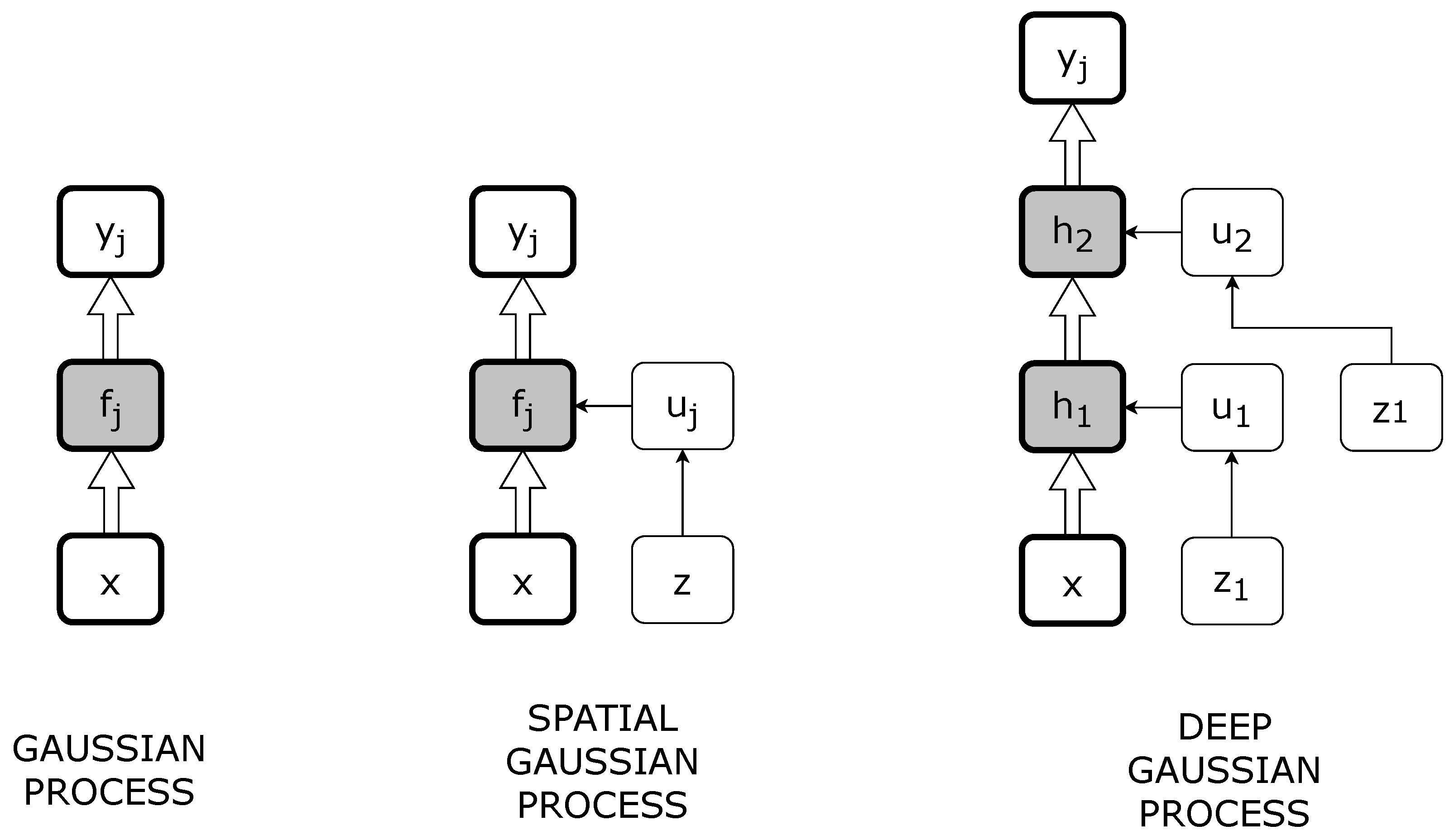
Other methods based on GP can be seen in the approach presented in [26]. Of course, the authors solving the same problem of predicting the end of life time of the cells and SoH in general, but in a very different manner. They propose deep Gaussian Process variations, which use GP to model mapping between layers, and matrix-variate Gaussian distribution to model the correlation between nodes of a give layer [26]. That allows to estimate the capacity of the cell using partial charge-discharge time series data (voltage, current, temperature). It also eliminates the need for input feature extraction. The authors focused on a special GP variant known as the special Gaussian Process (SGP). SGP solves two problems of GP Regression: GPR accuracy dependence on the locations of training data points (its highly accurate near those datapoints) and computational complexity (of inversed kernel matrix). In SGP it is assumed that the training dataset is augmented with pseudo-inputs Z and the associated outputs $u=f\left(K\right)$. SGP has been also extended by Damianou and Neil [28] to deep Gaussian Process Regression. The main idea is to use the l layer as on input to the $l+1$ layer. Both SGP and DGPR concepts can be seen in Figure 1. DGPR in fact is created by stacking some SGPs on top of each other. Layers between first input and last output are called “hidden”.

The last reviewed approach in [27] focuses on searching and estimating a special moment in the battery life cycle called “knee point”. The algorithm is also different as it consists not only of the Gaussian Process but is also augmented with feature extraction and selection modules. The authors point out that not all batteries behave just like those from the provided datasets so the knee point can happen in different points that could be assumed. The proper indication of knee points is important in that it informs that the cell will soon need a replacement [27]. There also exist some other estimation methods (for instance approaching 80% of capacity), but they are mostly based on other searching principals such as point estimations instead of whole transients. The whole idea presented in Figure 2 takes a special algorithm to extract features from the datasets (voltage, current etc.), select a relevant subset of key features and finally feed the Gaussian Process regression model with it. The output should be a capacity fade trajectory estimation [27]. GP was poorly conditioned by initial settings. The hyperparameters were fitted to the training data in the standard way using maximum marginal likelihood estimation. The kernel was set to the Matérn 2.5 function, because of previous research in [24,25], where it has been shown that it works well. Moreover, contrary to previous examples, the authors used different datasets in their research. The general conclusion is that the whole idea makes practical sense. The accuracy is about half a day of time for achieving knee point (or 2.6% across 600 predictions). They also used different subsets of data, but it turned out that the more the better. Overall, the information on how all different features correlate with each other is extremely viable with the use of the accurate forecast of capacity, end of life and the knee point. Moreover, they suggest that the problem should still be developed for other approaches and deeper research of data correlation.

5.2. Electricity Usage and Generating Prediction

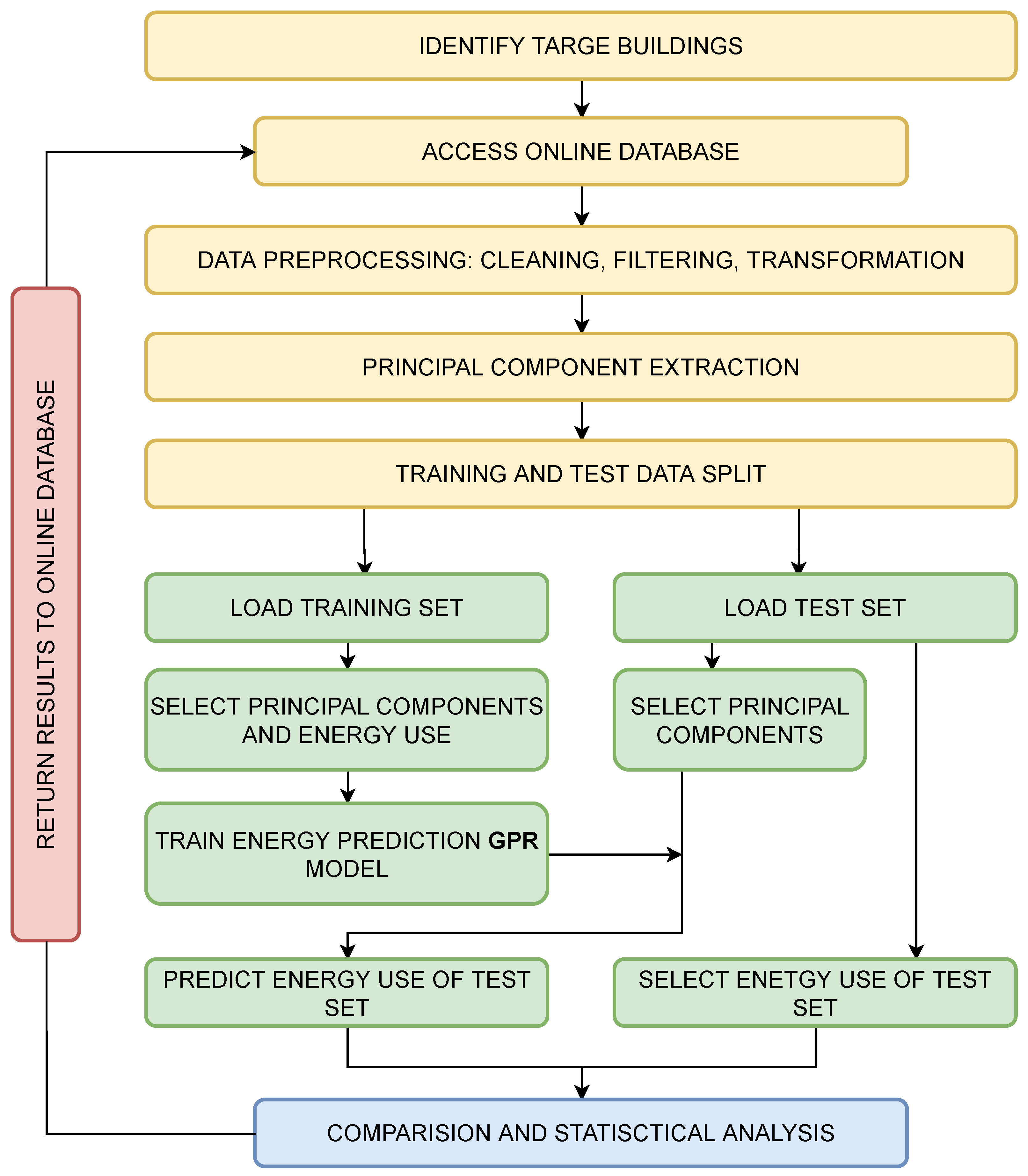
Nowadays, more and more devices and structures use electricity, so the prediction of its usage can be an important matter especially in terms of smart cars or smart homes where it can be both a matter of proper operation and of huge savings. The same principles guide the authors of [29], where the main aim is to predict energy consumption by different kinds of buildings which can lead to optimizing it through special control and low-energy strategies.

General workflow starts from collecting and preparing data, which comes from actual buildings. Being more accurate, from six different commercial buildings and its energy use database. The principal parameters were chosen by taking into account their impacts on the building electricity use. Those impacts were measured by calculating the correlation between energy use and meteorological parameters. The authors also considered users’ behavior. Then the whole set was filtered, cleansed and parsed in order to be used to predict the electricity usage [29].

GP regression is used as the prediction algorithm. The authors claim that, compared to the popular support vector machine (SVM) method, GPR shows great advantages in learning the kernel and regularization parameters, integrated feature selection, and generating fully probabilistic predictions. The model treats the occupancy schedule and the meteorological parameters as inputs. The output is building energy consumption. GP models were trained on a training dataset, and the model gives a numeric value of energy use of the test dataset based on the known inputs. The whole framework is shown in Figure 3 [29].

Data used in the creation and validation of model came from shopping malls, offices and hotels. The statistical analysis of results were conducted by authors. They calculated Root Mean Squared Error (RMSE) as well as Normalized Mean Bias Error (NMBE) and R-square to catch the accuracy of the model’s prediction. Conclusions were that GPR was regarded as a very accurate way of predicting the energy usage in this case study. It also generates predictions in very limited CPU time (at around 0.02 s per prediction). GPR can catch different energy patterns and can be used with very different inputs such as weather conditions, occupancy activities and others. Moreover, the authors claim that GPR can also be used with problems connected to predictions of the thermal dynamics of buildings and variable operations. In addition it could be compiled with a control system based on deviation of prediction.

On the other hand, GP can also be used for power generation prediction. In [30] we can see the comparison of some methods used for the prediction of the wind turbine power curve (WTPC). WTPC is a characteristic of the turbine which shows the relationship between output power and wind speed. Stochastic and intermittence exist in the generated wind power, which affect the safety of the power grid. The prediction of wind power is also very critical in wind power dispatching and even in enhancing wind turbine controllability [30]. Methods chosen by authors to predict WTPC are as follows:

• Gaussian Bin method;
• kernel density estimation (KDE);
• conditional kernel density estimation (CKDE);
• conditional probability via Copula;
• relevance vector machine (RVM);
• and of course Gaussian Process Regression.

In this review, we will focus only on GPR usage and its results in this problem. The whole process of setting up GP lacks a detailed description. Hyperparameters of coviariance functions are obtained by maximizing the marginal likelihood. The authors also notice that GPR is adopted for WTPC modeling, so both point estimation and confidence intervals can be calculated. Interval modeling was based on a brief description in [31]. The main issue with GPR is computational complexity, which is unfeasible for large datasets. Results differ amongst all methods and depend on what was to be accomplished. GPR was best for modeling efficiency and is suitable for online estimation and can be applied in super-short-term or short-term wind power prediction. Statistical models (Gaussian Bin, KDE, Copula) can be used in offline estimations as operational performance evaluation of wind turbines or wind farms [30].

6. Decision Support for Bike-Sharing System

Bike-sharing systems are widely used across the globe especially in major cities. Their main use is in improving healthy and convenient transport for citizens. People can just rent a bike at any station and return it at any other. The significant problem with this system is the high usage of single stations which results in a lack of bikes or not enough free docks to return one. System operators try to solve it by reacting in real time to high demand and manually repositioning bikes between stations. This solution cannot properly handle this problem as it is always too late to make an action after the jammed station was observed [32]. 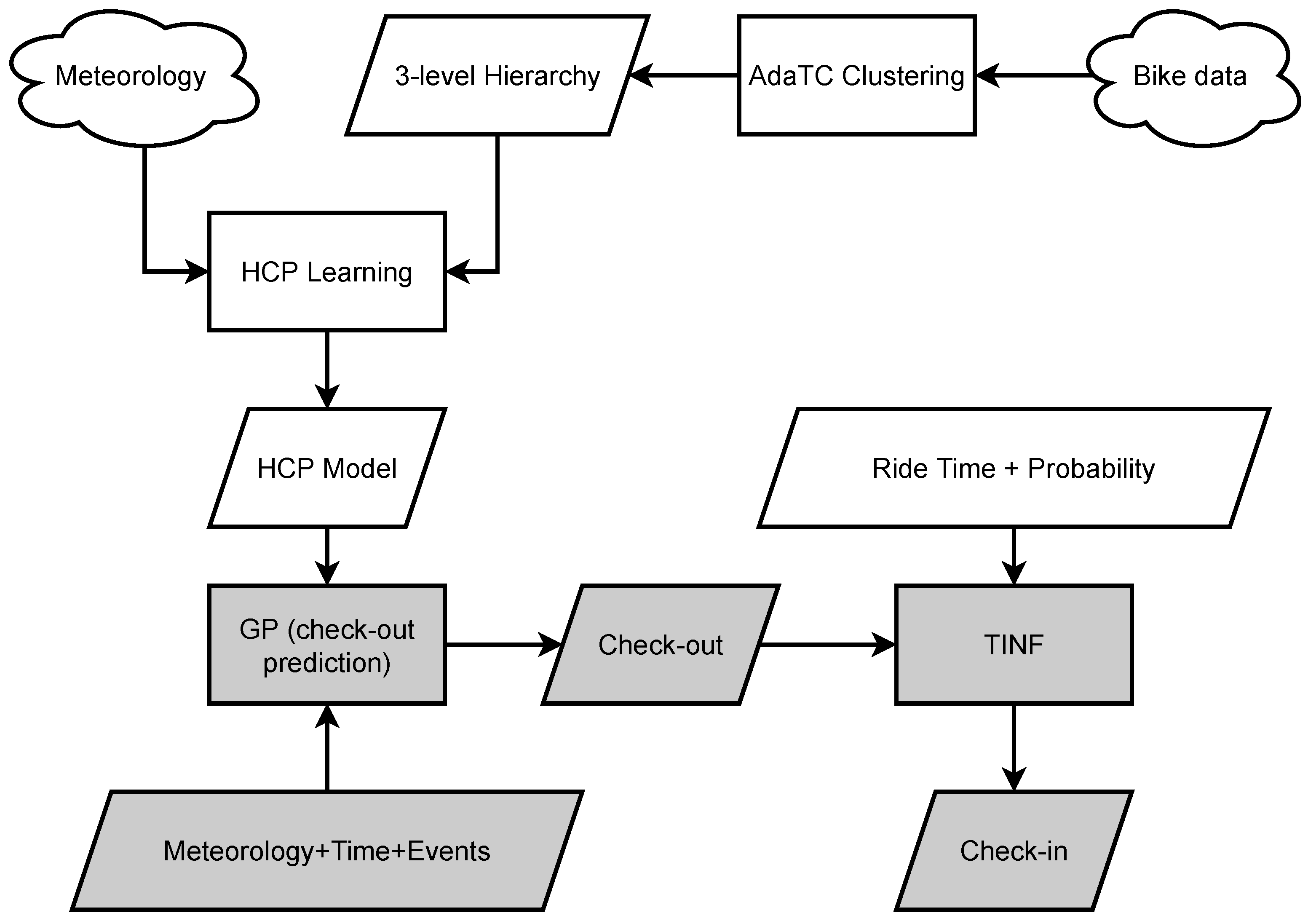To efficiently operate such a system, the authors of [32] proposed a complex model to predict citywide usage of bikes in the near future which allows the prevention of problems before they occur. The whole proposition of Hierarchical Consistency Prediction (HCP) consists of:

• Adaptive Transition Contraint (AdaTC)—which is a clustering algorithm used to cluster station into groups. This makes the rent and transition more regular within each cluster;
• Similarity-based Gaussian Process Regressor (SGPR)—which is a variation of GP used to predict how many bikes will be rented in different scale locations (e.g., single station, cluster etc.);
• General Least Square (GLS)—which is used to collectively improve obtained predictions;
• Transition based Inference (TINF)—which is designed to infer citywide bike return demand on predicted rent demands.

Figure 4 shows a whole framework which includes all mentioned parts. First, the AdaTC clusters’ whole data based on station locations and bike usage patters. Then 3-level hierarchy model (HCP) is formulated. SGPR is used to make a check-out prediction based on available data and GLS improves it to final check-out form. At the end, the TINF method impact system is used with check-in prediction [32].

For us the most interesting part is the usage of Gaussian Process variation. The authors started with the use of the basic GP regression model, with the most common settings:

$$\mu \left(f\right)=0$$

(24)

$$\kappa \left(f_1,f_2\right)=a^2\times exp\left(-{\sigma }_4^{-2}\times {\left(f_1-f_2\right)}^2\right),$$

(25)

where $\mu$ is mean, $\kappa$ covariance function and $a,\sigma$ are parameters. Then to a specific location the M-similar matrix training set in a target period $f_{t+1}$ is created:

$$H_{t+1}=\left\{\left(f_1^{t+1},x_1^{t+1}\right),\left(f_2^{t+1},x_2^{t+1}\right),\dots ,\left(f_M^{t+1},x_M^{t+1}\right)\right\}.$$

(26)

SGPR is an extension of GPR, which allows us to predict the value of function in $f_{t+1}$ in a certain location based on $H_{t+1}$. The authors also base some formulas on [1]. SGRP hyperparameters are learned by minimizing the total regression error on its validations set. Taking into account the specify of every locations, the authors learnt SGPR separately for each of them. Otherwise, the prediction accuracy could be negatively impacted [32]. In conclusion, GP was used in a slightly different form in order to adapt it to the problem, but overall usage was the same as usual. To sum up, the authors conducted a series of tests on real data which confirmed the effectiveness of their model, and they would like to generalize the model in the future.

In [33] we encounter a similar problem of bike-sharing difficulties connected to high-demand on stations. In addition to a general solution, they take into account the limiting effect of supply on demand. In order to accomplish that, the authors propose to implement censored likelihood which is able to train supply-aware models. In addition, the Gaussian Process model is used for time-series analysis of bike rentals, in order to calculate bike-sharing demand prediction. Both solutions are combined together to obtain satisfactory results.

The censoring problem was implemented, referring to the Tobias model [34], which can be simplified to: for each observation i, the model assumes that there is a latent (e.g., unobservable) variable $y_i^{*}$ and an observable censored realization $y_i$. The real demand is represented by $y_i^{*}$ while the available historical observations are represented by $y_i$. The simple form of the Tobit model is a dependency of variables on input data x in a linear relationship with parameters $\beta$ with the addition of error ${\epsilon }_i$, which we assume to be normally distributed (Formula (27)) [33].

$$y_i^{*}=\mathit{\beta }{\mathit{x}}_i+{\epsilon }_i,{\epsilon }_i\sim N\left(0,{\sigma }^2\right).$$

(27)

The Gaussian Process, as mentioned before, is used for the prediction of demand. The authors note that, one of the most important values which comes from GP is not only the prediction on its own, but also its confidence interval. They also focus on three different kernels: Squared Exponential Kernel (SE), Periodic Kernel, Matérn Kernel, which are used in the project. Moreover, the optimization methods based on the maximizing likelihood, which was mentioned earlier in this review, were used to optimize hyperparameters [33].

What distinguishes this approach is combinations of GP and censoring problem, which gives us Censored Gaussian Processes (CGP). CGP have to deal with a censored regression problem and simultaneously be able to exploit GP flexibility to fit complex patters. It can be done by defining a censoring-aware likelihood within a GP framework, using it instead of standard GP likelihood. At the end, experiments on datasets from Donkey Republic (bike-sharing provider in Copenhagen) were conducted. Results showed that taking into account the limiting effect of supply on demand is very important for creating an unbiased predictive model of user demand behavior. Moreover, GP is considered a great way to solve a problem, because of its capability of representing an elegant framework which is able to work in a fully probabilistic way and to deal with uncertainty in predictions [33].

7. Gaussian Process in Tracking Problems

Gaussian Process Regression finds its usability in some kind of tracking enhancment. For instance in [35], GPR is used to reconstruct the trajectory from the recorded location samples. The whole idea base for the application was called SensTrack. The creators of the application claim that more and more smartphones are equipped with powerful sensors such as GPS, WiFi, acceleration and orientation sensors, so all of them can be used to enhance the tracking of devices, for instance in areas with no GPS signal such as indoors, and most importantly to reduce the energy consumption overall (because constant GPS usage drains the battery) [35].

SensTrack smartly chooses the location sensing method between WiFi and GPS, and also reduces the sampling rate by using data from other sensors: acceleration and orientation. Data collected this way are analyzed and filtered to reconstruct a user’s original trajectory with GPR. Critical locations, decided by the sensor hints, which captures most of the key features of trajectory, were taken for a training set of GPR. As a test set—predicted locations between the successive but faraway location samples were used. The authors used standard settings of GPR: mean equals 0, for notation simplicity, and kernel functions of square exponential one. The real-world paths were examined and showed that SensTrack only needs 7% GPS samples of the naive approach and saves nearly 90% GPS activated time, while still reconstructing the original trajectory with high accuracy and coverage [35].

The authors of [35] also created an equivalent of SensTrack, the main purpose of which was for use in the Internet of Things (IoT) [36]. The IoT concept consists of Internet-connected devices with computing capability and have an ability to share data over the Internet wirelessly [37]. The main principals are the same, but the overall project here is in an earlier state. Most of the assumptions there are connected to GPR based on other work [38], which is in fact written with the use of machine-learning principals created by Rasmussen [1], so it concentrates all means of the machine-learning approach, as many of the other examples cited in this review.

The other kind of track problem, without actual use of GPS, is in [14]. Here, we encounter a problem of indoors tracking (which is the reason for the no-GPS approach). Contrary to other solutions, the authors did not base it on WiFi, Ultra Wide Band, Bluetooth nodes or similar. The whole 2D tracking algorithm is based on localization technologies, which use artificial light signals to substantiate positioning. Several methods to obtain such positioning exist: Received Signal Strength (RSS), Angle of Arrival (AoA), Time of Arrival (ToA) and Time Difference of Arrival (TDoA). The authors focus on an RSS based strategy with the intensity modulation of light sources for illumination as a localization system. This technique is called the Visible Light Positioning strategy (VLP), which consists of some Light Emitting Diodes (LED) for the purpose of fixed transmitter beacons and a photodetector as a receiver sensor [14].

The main parts of the project are the VLP Propagation model and the GP model. In this review we will mostly focus on how GP was handled here. A detailed description of the VLP model can be found in [14]. In general, the main purpose of it is to get an estimate of the coordinates of the location. The authors note that to solve the data oriented RSS-based VLP regression problem, there are many methods available currently, but using GP can handle problems very well, because of being very data-efficient and having an automatic optimization of hyperparameters and regularization. The authors use the predefined RBF kernel, with each entry of the RSS-base input and set to mean value 0. The hyperparameters of the RBF kernel were calculated by maximizing the log likelihood of data. Of course, this approach provides us with prediction, as well as an uncertainty for function values in new points [14].

As a validation of the created approach, the authors gathered data in slightly different scenarios (for instance: changing the LED installation high). Then the multilateration and GP approaches were tested and the performance of each was calculated in terms of $p90$ and $p95$ errors. Generally, GP turned out to outperform other methods by any means, in each scenario. Moreover, the author notes that GP has an advantage when it comes to a higher installation for data gathering, which can implicate the future use of such a solution in, for instance, warehouses [14].

8. Various Optimization Problems

Apparently, GP can be used in solving various problem stating with simple regression to complex prediction or identification. Last but not least, we would like to show some different, unrelated to each other applications of GP, which mostly aim to optimize different processes.

8.1. Cost Optimization

First of all, in [39] we can see the optimization of the cost of creating the cloud data center. The problem consists of creating a project and a model of the mentioned cloud data center, taking into account things such as infrastructure, fault possibility etc. Data center main parts are: power, cooling, and IT. Each of these systems are described in detail. Then the project was divided into subsystems, which consist of simple blocks. Thanks to that it is possible to calculate the availability and to calculate the cost of the projected architecture. Then, the optimization is needed in order to find the best cost solution while taking into account the constraints. The authors used algorithms like Particle Swarm Optimization (PSO), Differential Evolution (DE) and Genetic Algorithms (GA) to achieve this goal [39].

Creating such a model, with many places, transitions, and tokens turns out to be extremely complex to compute. To reduce the complexity, and get rid of the heavy computing problem, the authors decided to use a surrogate model with the use of GP. Contrary to other proposed solutions such as neural networks, GP does not need a huge training dataset to be useful. They used a kind of GP called design and analysis of computer experiments (DACE), often referred to as kriging. In the original mean, kriging is a statistical interpolation method based on GP to interpolate complex functions. Moreover, kriging is used to represent the input/output mapping of expensive computational models. It is now also connected with problems such as regression and identification [40]. A sampling strategy of Latin Hypercube Sampling (LHS) was adopted in this case. The authors evaluated the surrogate to ensure a low error in comparison to the original model. Thy created different scenarios with:

• exponential covariance, optimization via genetic algorithms with a maximum of 1000 generations;
• with similar configuration, only changing the covariance to Gaussian;
• with Gaussian covariance and Broyden-Fletcher-Goldfarb-Shanno (BFGS) optimization method with 1000 start points.

The results of creating the surrogate model were satisfying, with low RMSE. The whole problem was also tested, but these results focus mostly on choosing which one from three presented optimizing algorithm performs best [39].

8.2. Diesel Engines

A completely different problem can be encountered in [41]. The main focus is on problems connected to diesel engines, more specifically post-injection models. Due to several factors, this method is already widespread and its importance will only grow. The main reason is ecology: the use of DPFs and the optimal selection of operating parameters is key to achieving a compromise between the pollutants produced and harmful NOx—we are dealing here with frequent DPF regeneration cycles, catalyst wear and cold start. All these factors contribute to the transfer of fuel to the oil. This causes the oil to dilute and, over time, makes it a necessity to be replaced (otherwise it will damage the engine). The described experiments are designed to find the optimal setting of parameters and types of post-injection of the engine in order to minimize oil dilution—this results in lower operating costs, etc. Additionally, the authors also take into account the automatic evaporation of the fuel [41].

The GP model is built on the basis of test data obtained on the basis of various scenarios of diesel engines. Then, on this basis, predictions are made as to the behavior of the oil in a given configuration. The authors look for correlations between factors and outcomes. The whole GP model was based on several sources [42,43,44], which exhaustively describe its application in this field. Studies also resulted in a comparison of GP to polynomial regression. It turns out that in engine related problems, GP outclasses polynomial regression. Overall, the results met the expectations of the authors, showing the relationships between various factors on the basis of several different sample tests. The GP was shown to be a good approach to the model formation rate of oil dilution [41].

8.3. Model Predictive Control

Many control problems are based on designing a stabilized feedback with minimized performance criterion which satisfies constrains of the controls and states. The best solution would be to look for a closed solution for the feedback. Unfortunately, often closed solutions cannot be found analytically. A known approach to solving this problem is the repeated solution of the open-loop optimal control problem in a specific state. So the first part of this open-loop result is implemented and then the whole process is repeated. A control approach that utilized this strategy is called model predictive control (MPC) [45].

The GP based model of predictive control is the main purpose of the [46] article. The authors propose that kind of solution, mostly because of the measure of confidence offered by GP. That feature is very helpful in non-linear MPC (NMPC) design. They also note that GP is a probabilistic non-parametric black-box model that provides information about prediction uncertainties, which are difficult to evaluate appropriately in non-linear parametric models. The whole GP was set based on complex and different approaches, which are feasible in order to create a model for NMPC. A detailed description can be found in the article [46].

The whole idea was implemented on the gas–liquid separation plant example. The results of this approach were successful. The authors note that thanks to the confidence interval, the GP model can highlight input spaces, where prediction quality is poor, for instance due to data complexity or lack of it. This is a very attractive feature in control design. The only drawback of this solution is a computational complexity for industrial purposes. For the presented case (model contained about 1000 points to identify), the calculation of covariance matrix inversion was time consuming. The model barely managed to keep time constraints, but as the authors say, it should not detract from the overall value of GP usage [46].

8.4. Image Processing

The last presented application of GP is from the field of image processing. The whole idea in this example is to use GPR for image time series fap-filling and crop monitoring [47]. Basically, the optimization problem here is mainly about optimizing the GPR itself for a better performance in this field, but it is still a very good example of its general application. GP proves to be a very competitive solution in the field compared to the others available, especially as it has an uncertainty band. However, its computative complexity is problematic especially in the per-pixel approach mainly for GPR training rather than the fitting step. The authors proposed their own solution to get rid of this burden.

The authors demonstrate different ways to accomplish GPR fitting. They start with the base of other attempts to use GP for image processing which have been successful such as in [48,49,50,51] and many more. The authors focus mainly on describing the process of setting up the model for their case. A kernel function called Squared Exponential deserves special attention, as it is the most commonly employed covariance function in this area as it reflects the prior beliefs of the problem. SE is described in detail in the work, especially by means of its parameters. The process of optimizing hyperparameters is maximising the log marginal likelihood.

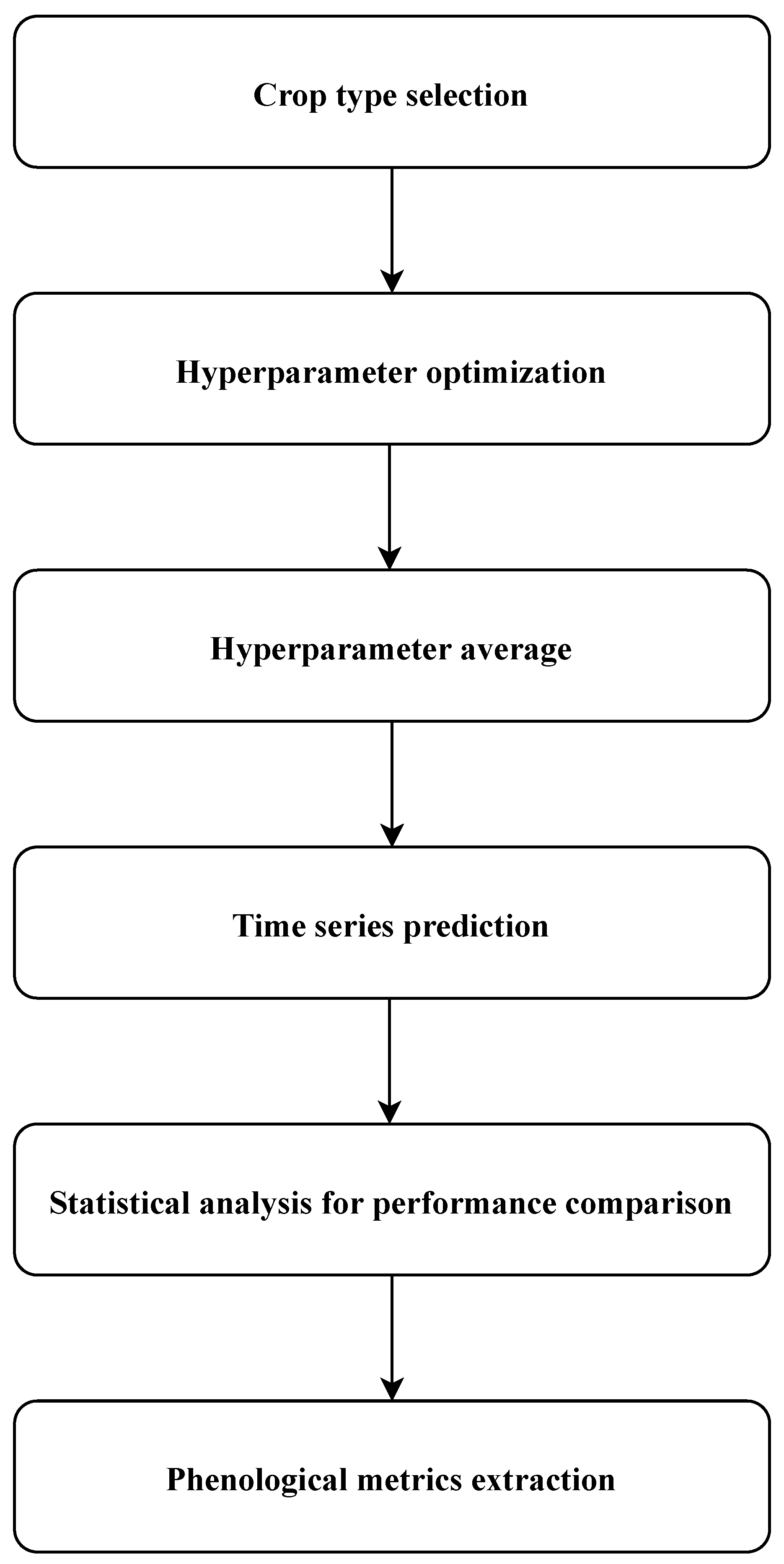
To mitigate the mentioned computational burden, the authors proposed to substitute the per-pixel optimization step with the creation of a cropland-based precalculations for the GPR hyperparameters. The whole process is shown in Figure 5 and consists of:

• Crop type selection: for each crop type found, select random parcels;
• Hyperparameter optimization: performed by assessing individually each pixel;
• Hyperparameter average: mean of the previously trained hyperparameters for each crop type—also global average is computed;
• Time series prediction: LAI-reconstructed time series computation with different GPR parameterizations;
• Statistical analysis for performance comparison: evaluation of the performance of the different GPR models in terms of reconstruction with RSME indicator;
• Phenological metrics extraction: analysis on how different GPR parametrizations affects estimations.

Overall, the results of this optimization are quite promising. The proposed method of the calculation of hyperparameters can be even 90 times faster, while being just slightly less accurate than non-reconstructed parameters. Moreover, the authors point out that GP is underutilised currently in time series processing and just some recent studies started to explore it in crop monitoring and as can be seen there is still room for GP to be researched in this field [47].

9. Discussion and Future Direction

As research shows, a significant part of the use of GP in various fields focus on being used based on testing several covariance functions, selecting accurate ones and using automated optimizing of parameters consists of maximising the log likelihood (ML-II method). Of course, such an approach is not fundamentally wrong. Its primary advantage is the ease of use, high flexibility and speed of operation. As mentioned in examples, we can see that it can be easily set up with various environments (e.g., Matlab or python packages). Users can just fill the program with data and easily fit it with an automated method of hyperparameters optimization. The only visible challenge here is the correct choice of kernel, almost always from an already defined base of covariance functions. With the high overall flexibility of GP usage, it can be a useful tool to solve a problem with the help of GP.

Besides that, there are more different approaches to GP. Some of them we mentioned in this review in the examples of use. In an article on the DT concept [20], the authors used another method of kernel choosing, which consisted of making a calculation on linear combinations of covariance functions and optimizing parameters in a different manner. One example with battery health parameters prediction [26] shows an extension of GP called SDGP, which is a “neural network patter” fix for some common GP problems known in this specific scenario; the same kind of solution as “extending” GP capabilities to the certain problem we saw in [33]—bike-sharing load prediction with censoring. The authors of [47] also managed to make GP more suitable for certain problems. Approaches such as this give overall better results not only in accuracy but also, e.g., in computing time.

Regardless of the chosen method, GP has a serious problem with the computation burden of covariance matrix inversion. The size of this matrix depends on the number of data considered in the problem. If there are too many of them, GP becomes unbearable while other methods become more appealing, especially from the machine-learning field while we encounter a lot of data. Of course, there are approximation methods, which helps to overcome this issue, but at an obvious cost of accuracy and sometimes unnecessarily complicate the problem, when one could just use methods other than GP. Moreover, solving GP analytically is often complicated, so there is always the necessity to use some sampling methods. Some optimizing methods have a problem with overfitting, low accuracy and bad generalization of use. Overcoming this challenge requires not only specific methods but also specific knowledge. In addition, it is worth noting that, if we cannot find a kernel matching our prior belief of the problem, it is really hard to create a new one. The task is so inconvenient that in most cases less appealing kernels are used, or the GP is dropped as a solution. These problems arise mostly when we are trying to solve some complex issues or they do not generally fit methods like GP, so everyone who tries GP in their research should be aware of that and if necessary reconsider using GP.

The whole paper shows a fragment of the GP world in control engineering, their practical application in specific areas and the ways of its implementation, as well as the results achieved. We can easily deduce two solid facts. First, GP is used in many fields related to control engineering, and with passing time, it is only gaining in popularity. Second, it is mainly used in the simplest and fully automated use that does not require complex modeling, knowledge and a lot of time. The second fact is where we can make further progress. Basically, there is nothing wrong with the most common use of GP. At a low cost, it shows whether the use of GP to solve the problem makes sense, or whether there are perhaps more appropriate algorithms. When such a problem seems to be ideal for the use of GP, such as detecting industrial anomalies or predicting battery life parameters, it is advisable to further develop and improve GP using available methods, e.g., by more accurate model creation, better hyperparamters optimization or better kernel matching (for instance by combining them). The development of GP does not stop on even presented approaches such as the Bayesian inference hierarchical model with MCMC sampling or approximation mentioned approximation methods. There are more methods, which develop values of Gaussian GP. For instance, we could use Gaussian Random Fields (GRF) in solving widely oriented control engineering problems, because GP is actually a one-dimensional GRF. In [52], the authors show the way of exploring this topic in spatial modelling. Another topic called Gaussian Process latent models, which generally attempt to capture hidden structure in high-dimensional data, can be an interesting direction as well. A more detailed review on GP latent models can be seen here [53]. Other interesting work related to the GP area can also be seen in [54,55].

Developing new strategies and applying ones which exist but are not currently commonly used in the field of control engineering is the direction which is highly suggested to be followed in terms of the future of GP.

10. Conclusions

Gaussian Processes are one of statistical modeling methods, which is rising in the popularity alongside Bayesian statistics in several recent years, despite that concepts of the GP were well-know to the scientist before. One reason of a such state is probably the computation burden of GP modeling connected mostly with the necessity of large covariance matrix inversion. The current state of technology allows us to use GP to a wider scale, but still more complex approaches require too much computation power than can be provided. For such cases, approximation methods of GP were developed. It can be noticed that most of the reviewed cases are still handing GP solutions with ML-II methods. However, it has to be said that more and more scientists are encouraged to develop more advanced approaches to solving problems with GP, even creating their own methods.

This review shows that GP has enormous potential when it comes to real-word control engineering applications. We can easily find a GP based solution in fields of anomaly detection (especially in industry), battery parameters and other electricity related prediction, image processing, expenditure planning as well as support for bicycle or location systems and others. We can classify the primary uses of GP as regression, identification, prediction, and classification. A certain correlation was noticeable: the more research examples we found in a given field, the more modified GP methods were encountered. This is probably due to the discovery of the potential of GP for a certain field and further willingness to improve these algorithms by other means.

The methods that can build more and more accurate GP models such as the hierarchical model with MCMC sampling involve following the direction to increase the usability of GP. With too complex problems in terms of computation, some approximation should be involved. The first step for the future of GP is to involve more complex methods (different from the mainstream, not only those described here) for resolving problems, which will give us an advantage in solutions over the currently dominant methods. The major result of this review paper is an orientation on the current state of use in the areas and methods of using GP in related fields with broadly understood control engineering and providing a future direction and tips on where to develop the field further.