Hadamard Aperiodic Interval Codes for Parallel-Transmission 2D and 3D Synthetic Aperture Ultrasound Imaging

Abstract

We present a new set of near orthogonal codes which we call Hadamard Aperiodic Interval (HAPI) codes and demonstrate their utility for parallel multi-transmitter synthetic aperture imaging. The codes are tri-state and sparse. Locations of non-zero bits are based on marks in a sequence of aperiodic intervals, also known as a Golomb ruler. The values of non-zero bits are selected from Hadamard sequences that are mutually orthogonal. This ensures that cross-correlation sidelobe magnitudes between differing codes are bounded by unity while the autocorrelation approaches a delta function with mainlobe-to-sidelobe levels scaling with the number of non-zero bits. We use simulations to demonstrate the potential of the codes for synthetic aperture imaging. A multiplicity of transmitter elements is used to transmit codes simultaneously, with a different code for each element. Echo signals are received from a multiplicity of transducer elements in parallel. Channel data from each receiver element are cross-correlated with respective HAPI codes to estimate the transmit–receive signature associated with each transmitter–receiver pair while minimizing crosstalk. This estimate of the full transmit–receive synthetic aperture dataset is then used to form high-quality images demonstrating image quality and signal-to-noise ratio improvements over multiple flash angle imaging and synthetic aperture imaging methods for linear arrays. We also demonstrate simulated full volume synthetic aperture imaging with random sparse arrays, possible with one extended HAPI code-set transmit event.

1. Introduction

Most ultrasound imaging systems transmit the same waveform on each array element with some electronically programmable delays and apodization weightings. New imaging possibilities may open up if different coded excitations could be transmitted from different elements in parallel. Ideally, these codes would be mutually orthogonal in the sense that their cross-correlation is negligible and their autocorrelation approaches a delta function, so that decoding could be performed with minimal crosstalk. Codes which satisfy these conditions are difficult to find.

Various forms of coded excitation have previously been explored in the ultrasound imaging literature. Barker codes are one type of binary code [1] that are most commonly used in communications due to their cross-correlation properties [2,3,4,5]. These codes are considered to have good cross-correlation properties because their autocorrelation function produces a peak of N, where N is the number of code elements in the code, and a sidelobe level bounded by a minimum value. Barker codes of length 13 have been shown to produce an SNR increase of 11.1 dB over conventional pulse-echo imaging [6]. However, Barker codes of lengths greater than 13 have yet to be found [7], and at this maximum code length, Barker codes will not produce the high dynamic range >50 dB typical of most ultrasound imaging systems, even with Wiener-filter deconvolution.

Golay codes are another type of binary code that are used for increasing SNR and for improving penetration depth in ultrasound imaging [8,9,10]. They are pairs of binary codes belonging to a set of codes called complementary codes [11]. These complementary codes consist of two codes of length N, whose autocorrelation function have sidelobe levels equal in magnitude but opposite in sign. When the autocorrelation functions of the complementary codes are added together, they result in a composite autocorrelation function that has a mainlobe peak of 2N and sidelobe levels of zero. The sidelobes completely cancel out because they are equal but opposite in sign. This means Golay complementary codes produce an ideal autocorrelation function which is essential for imaging with good quality. Golay codes have been successfully used to image and have shown an increase in SNR of 32 dB over sine burst excitation [12].

Binary codes such as Barker codes, Golay codes, and others are good for increasing penetration depth and signal-to-noise ratio, but they do not constitute a near orthogonal code set, and hence cannot be used for parallel transmission in ultrasound imaging. Orthogonal codes have been investigated for use in multi-user communications [13,14,15] and are successfully used in radio communications technologies such as CDMA (code division multiple access) [16,17]; however, most of these are meant for synchronous coded information transfer rather than high dynamic range imaging. The imaging problem can be considered asynchronous because locations of scatterers and hence echo-time delays are unknown and different for an ensemble of scatterers.

Two main types of orthogonal codes that are commonly used for asynchronous communications but are not commonly used in imaging are pseudorandom codes [18,19,20,21] and Kasami codes [22,23,24]. The sidelobe levels in the autocorrelation function of Kasami codes are small compared to the peak but are not guaranteed to be bounded by a minimum level. Kasami codes are specially constructed binary sequences with good cross-correlation properties. Unlike other orthogonal codes, the small Kasami code set meets the Welch lower bound [25]. The Welch bound is a lower bound on how small the cross-correlation and autocorrelation can simultaneously be at non-zero lags [26].

In the field of medical imaging, R. Chiao et al. showed through simulations that using spatio-temporal encoding with orthogonal Golay code sets could increase SNR by 10log(ML), where M is the number of transmit events and L is the code length [27]. While this paper by R. Chiao used Hadamard encoding to construct orthogonal code sets, recently another paper by Gong et al. used a delay-encoded transmission scheme to recover the synthetic transmit aperture dataset. This was conducted by delaying selected transmitting elements by a half period of the ultrasound wave relative to the rest of the transmitting elements [28]. The authors achieved a 7 dB improvement in peak signal-to-noise ratio over traditional synthetic transmit aperture imaging.

Most codes designed for multi-user synchronous or asynchronous communication applications require only that detected signal-to-noise and signal-to-crosstalk after decoding is sufficient to reliably detect binary bits. However, imaging applications require more stringent demands. Ultrasound imaging typically has a >50 dB display dynamic range and it is desirable that crosstalk is below this level or as low as possible. To ensure mainlobe-to-sidelobe levels after decoding are sufficiently high, very long pseudorandom or Kasami codes would be required.

Additionally, most codes in the communications literature are purely binary (+1, −1) or sometimes multi-phase. In ultrasound imaging, however, there is no need to restrict levels to binary states and in fact binary states of +1 or −1 would mean the transmitter is always on, which is the case for many communications devices. In ultrasound imaging, having the transmitter always on could lead to ultrasound thermal index safety concerns for medical applications. Considering arbitrary-level codes could open up new possibilities for the design of near orthogonal codes.

We introduce a set of novel tri-state codes which we call Hadamard Aperiodic Interval (HAPI) codes. The codes are constructed by creating a sequence of bits which take values of 0, 1, or −1. Tri-state pulsers are common on some ultrasound systems because of the simplicity of the electronics over arbitrary function generator capabilities. Locations of non-zero bits are constructed based on marks in an aperiodic interval sequence, also known as a Golomb ruler [29,30]. The values of non-zero bits are selected from columns of Hadamard matrices that are mutually orthogonal. This ensures that cross-correlation between differing codes is bounded while the autocorrelation approaches a delta function with mainlobe-to-sidelobe levels scaling with the number of non-zero bits. We demonstrate the utility of these HAPI codes for high-quality 2D and 3D ultrasound imaging using simulations of a scattering phantom with hypoechoic and hyperechoic regions. We demonstrate signal-to-noise and contrast-to-noise advantages over synthetic aperture approaches as well as other imaging techniques using linear array transducers. We also demonstrate the utility of our HAPI codes for fast 3D imaging using 2D sparse arrays.

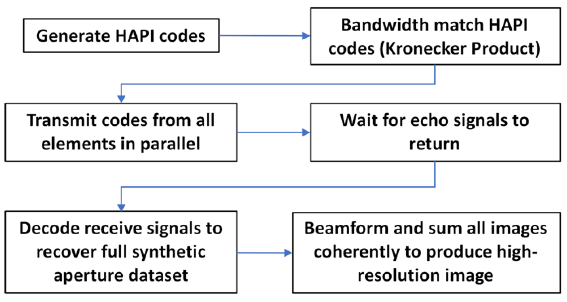
2. Materials and Methods

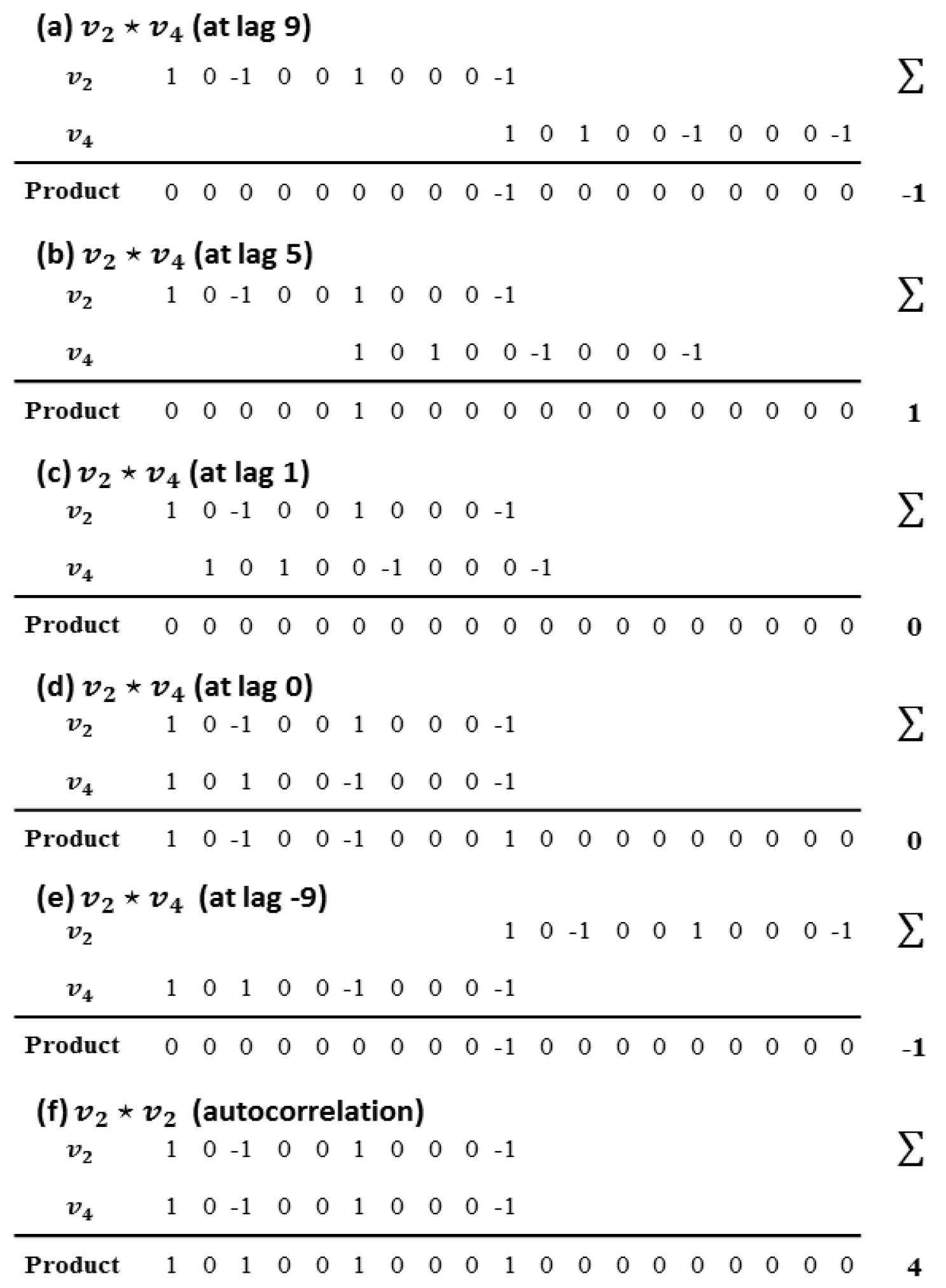
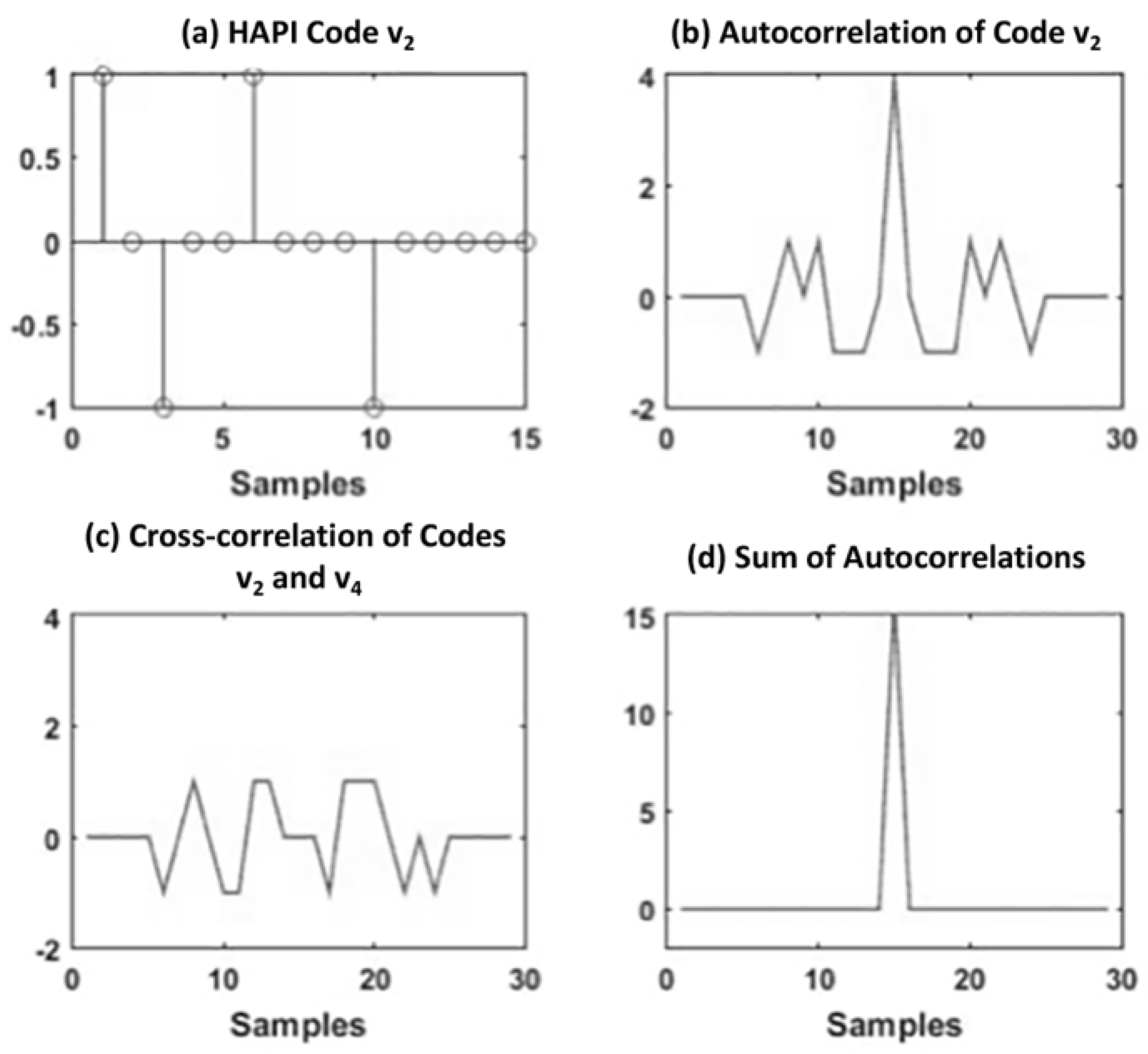
2.1. Mathematical Modeling Framework

In order to acquire a set of synthetic transmit–receive aperture data with one transmit event, we desire a set of codes such that a different code can be transmitted from a set of transmitters and then received signals from a set of receivers can be decoded for each transmit code with minimal interference between signals after decoding. We create a modeling framework for ultrasound imaging in this section; however, this analysis is valid for any multi-transmitter multi-receiver system.

First, consider an array of N transducer elements. The driving voltage signals of all elements can be represented as Equation (1).

$$\mathit{V}\left(t\right)=\left[\begin{array}{cc}\begin{array}{cc}{v}_1\left(t\right)& v_2\left(t\right)\end{array}& \begin{array}{cc}\dots & v_N\left(t\right)\end{array}\end{array}\right]$$

(1)

where $v_N\left(t\right)$ is the voltage as a function of time driving element n, which can be represented in its discrete form as a vector of M time samples, $v_n={\left[\begin{array}{cc}\begin{array}{cc}{v}_{n1}& v_{n2}\end{array}& \begin{array}{cc}\dots & v_{nM}\end{array}\end{array}\right]}^T$.

We want to transmit a set of codes such that the cross-correlation between different sequences is close to zero, and the autocorrelation is approximately a delta function (Equation (2)):

$$v_n\left(t\right)\star v_m\left(t\right)\approx {\delta }_{nm}\left(t\right)=\{\begin{array}{c}0 if n\ne m\\ \delta \left(t\right) if n=m \end{array}$$

(2)

where $\star$ is the autocorrelation operator and $\delta \left(t\right)$ is the delta function.

The received signal due to an ensemble of scatterers on receiver element k is given as Equation (3).

$$r_k\left(t\right)={\displaystyle \sum }_{l,j}{v}_l\left(t\right)\ast h_{Tx}\left(t,{\mathit{x}}_l\to {\mathit{x}}_j\right)\ast s\left(t,{\mathit{x}}_j\right)\ast \frac{\partial }{\partial t}{h}_{Rx}\left(t,{\mathit{x}}_j\to {\mathit{x}}_k\right)$$

(3)

where $r_k\left(t\right)$ is the signal due to an ensemble of scatterers at location ${\mathit{x}}_j$ using elements at location ${\mathit{x}}_l$ to transmit, $v_l\left(t\right)$ is the driving signal for elements at location ${\mathit{x}}_l$, $h_{Tx}\left(t,{\mathit{x}}_l\to {\mathit{x}}_j\right)$ is the transmitter spatio-temporal impulse response, $s\left(t,{\mathit{x}}_j\right)$ is the scatterer response at location ${\mathit{x}}_j$, $h_{Rx}\left(t,{\mathit{x}}_j\to {\mathit{x}}_k\right)$ is the receiver spatio-temporal impulse response, and $\ast$ is the cross-correlation operator.

If effectively orthogonal transmit sequences are used, we can estimate the signal transmitted from element m and received on element k$, r_{mk}\left(t\right)$, by cross-correlating the receive signal $r_k\left(t\right)$with $v_m\left(t\right)$ as shown in Equation (4):

$${\widehat{r}}_{mk}\left(t\right)=r_k\left(t\right)\star v_m\left(t\right)\approx {\displaystyle \sum }_{l,j}{h}_{Tx}\left(t,{\mathit{x}}_m\to {\mathit{x}}_j\right)\star s\left(t,{\mathit{x}}_j\right)\star \frac{\partial }{\partial t}{h}_{Rx}\left(t,{\mathit{x}}_j\to {\mathit{x}}_k\right)$$

(4)

We can then obtain an estimate of the full synthetic aperture data for all elements. Then, transmit–receive synthetic aperture delay and sum focusing can produce high spatial resolution and high contrast-to-noise images.

We desire tri-state codes of len gth M with states {−1, 0, 1} which satisfy minimal correlation and orthogonality conditions with the constraints:

$$\begin{gathered} \left|{\rho }_{nm}\left(\tau \right)\right|\le 1 \forall \tau if n\ne m \\ {\rho }_{nm}\left(0\right)=0 if n\ne m \\ {\rho }_{mm}\left(0\right)=M \forall m \end{gathered}$$

where ${\rho }_{nm}\left(\tau \right)$ is the cross-correlation between $v_n\left(t\right)$ and $v_m\left(t\right)$ at time-lag $\tau$.

With these constraints, the mainlobe-to-sidelobe ratio will be equal to M, and the sidelobe levels will be bounded for any code length.

In addition to these requirements, we further would like the set of codes to satisfy the following conditions (Equations (5)–(7)) to enable a set of transmissions to reproduce delta function cross-correlations:

$${\displaystyle \sum }_{m=1}^M{v}_m\left(t\right)=\delta \left(t\right)$$

(5)

$${\displaystyle \sum }_{m=1}^M{v}_m\left(t\right)\star v_m\left(t\right)=\delta \left(t\right)$$

(6)

$${\displaystyle \sum }_{m=1}^M{\displaystyle \sum }_{n=1}^M{v}_n\left(t\right)\star v_m\left(t\right)=\delta \left(t\right)$$

(7)

The next two sections discuss a novel way to construct tri-state codes that conform to such conditions, and show a simple example of the construction of a 4 non-zero bit HAPI code.

2.2. Constructing Simple HAPI Codes

In order to construct Hadamard Aperiodic Interval codes, varying sequences of zeros are interposed between non-zero bits obtained from a Hadamard sequence. The aperiodic interval sequence is based on a so-called Golomb ruler. A Golomb ruler is a set of marks at integer positions along a ruler such that no two pairs of marks are the same distance apart. The number of marks on the ruler is its order. Codes designed in this manner can ensure that a maximum of one pair of non-zero bits would multiply in a cross-correlation of two codes at any given lag, which produces an outcome that is bounded by unity. In addition, the autocorrelation of any code at zero lag will produce a value equal to the sum of the square of the bits of the Hadamard sequence, or M for an M-bit Hadamard matrix.

The following example illustrates how to build a simple 4 non-zero-bit HAPI code.

In order to construct a 4-bit HAPI code, we require 3 non-repeating intervals of zeros to interpose between the 4 non-zero bits. If we start with intervals of 2 and 3, we can pick a third interval, 4, which is not a combination of 2 and 3. Hence, our chosen intervals are {2, 3, 4}.

Next, we can construct four HAPI codes by interposing the non-zero bits sampled from each row or column of a 4 × 4 Hadamard matrix with the intervals of zeros chosen above.

The 4 × 4 Hadamard Matrix is given as

$$H=\left[\begin{array}{cc}\begin{array}{cc}+1& +1\\ +1& -1\end{array}& \begin{array}{cc}+1& +1\\ +1& -1\end{array}\\ \begin{array}{cc}+1& -1\\ +1& +1\end{array}& \begin{array}{cc}-1& +1\\ -1& -1\end{array}\end{array}\right]$$

For this example, we chose to sample each Hadamard sequence from each row of the matrix. However, we could have chosen to sample our bits from the columns of the matrix instead because both rows and columns of a Hadamard matrix are mutually orthogonal to each other. We can then interpose the sampled non-zero bits from the rows of this matrix with the sequences of zero intervals to construct four codes, as shown in

Table 1. Table of the four non-zero-bit HAPI codes derived from the rows of the 4 × 4 Hadamard matrix.

v1	1	0	1	0	0	1	0	0	0	1
v2	1	0	−1	0	0	1	0	0	0	−1
v3	1	0	−1	0	0	−1	0	0	0	1
v4	1	0	1	0	0	−1	0	0	0	−1
Intervals	2			3			4
	5
				7
	9

.

Table 1 shows the four HAPI codes we can generate from the rows of the 4 × 4 Hadamard matrix. The table also shows our chosen intervals of {2, 3, 4} and the combination of these intervals, {5, 7, 9}, shaded underneath. If we were to add one more non-zero bit, and thus require one more interval, then that interval cannot be chosen from the list of combinations {5, 7, 9}. Hence, our intervals of {2, 3, 4} are correctly chosen such that there are no repeating intervals or combinations of intervals.

Now, let us examine the autocorrelation properties of these codes and the cross-correlation properties at various lags.

Figure 1 shows the cross-correlation of codes $v_2$ and $v_4$ at every lag, and the autocorrelation of code $v_2$ to demonstrate that cross-correlation is bounded by unity for every lag, and that the autocorrelation is a delta function. We can see from Figure 1a–e that for any lag, the cross-correlation is bounded by unity, i.e., the result of a cross-correlation at any lag will be in the set [−1, 1]. The bounded property of the cross-correlation can be visually seen in Figure 2c below.

Figure 1f shows that the result of the autocorrelation of code $v_2$ is 4, which is the size of our 4-bit Hadamard sequence. Figure 2b shows the temporal representation of the result of the autocorrelation of this sequence. Furthermore, if the autocorrelations of all the codes $v_1$ through $v_4$ are added together, an ideal delta function is produced, as shown in Figure 2d.

2.3. Algorithm for Constructing Arbitrary-Length HAPI Codes

In order for HAPI codes to be useful, they must be much longer than only 4 non-zero bits as shown in the example above. A list of shortest-length Golomb rulers (also known as Optimal Golomb rulers) is only known up to order 27 [31]. Hence, we propose the following algorithm to construct arbitrary-length Golomb rulers and associated HAPI codes.

The algorithm starts with a seed sequence such as $S=\left\{2, 3, 4\right\}$, the same sequence that was used in the example above. The seed sequence can be any set of intervals such that no intervals or combinations of intervals are repeating. Additional aperiodic intervals are then added to this list for each non-zero bit that needs to be added. To add an additional aperiodic interval $n$ to append a new data bit with $n-1$ interposed zeros, we must search for an interval with the following conditions.

C1. The new interval $n=I_{k+1}$ should not be in the set of pre-existing intervals, $n\notin S_{excl},$where $S_{excl}=\left\{I,\{{\displaystyle \sum }_1^i{I}_k\forall i\in \left[1,2,\dots ,K\right]\},\{{\displaystyle \sum }_1^k{I}_{K-k}\forall k\in \left[1,2,\dots ,K\right]\}\right\}$ and$K=\left|I\right|$ is the cardinality or size of the set of intervals, $S=\left\{I_k,k\in \left[1,2,\dots ,K\right]\right\}$.

C2. Newly formed intervals (formed when combining the new interval $n=I_{K+1}$ with other pre-existing intervals) should not be in the set of excluded intervals: $n+b\notin S_{excl} \forall b\in B$, where $B=\{{\displaystyle \sum }_1^k{I}_{K+1-k}\forall k\in \left[1,K\right]\}$ is the set of intervals terminating at the right-hand side of the existing sequence.

The newly added interval should be of minimum possible length for maximum compactness. but this is not essential. We then add the new interval to the ordered set of HAPI intervals $S$ and update the sets $S_{excl}$ and $B$.

Following these conditions, the proposed algorithm for generating the non-repeating intervals is then:

• Begin with a seed sequence of intervals, such as S = {2,3,4}.
• Search for a new interval that satisfies the criteria C1 and C2 above.
• Add the new interval into the ordered set S and update the exclusion set S_excl and the terminating set B.
• Iterate steps 1 to 3 until the ordered set S is of the desired length.

The only restriction is that for HAPI codes sampled from Hadamard sequences, the desired length should be a power of 2.

For example, in the case of the 4-bit HAPI code example, the exclusion set $S_{excl}=\left\{2, 3, 4, 5, 7, 9\right\}$ and the terminating set $B=\left\{4, 7, 9\right\}$. Hence, if we wanted to add one more non-zero bit and so one more interval to the list, we could choose an interval that is not in $S_{excl,}$ such as 6.

Once the intervals are generated by the above algorithm, HAPI codes are then constructed by creating vectors of non-zero bits sampled from the different rows or columns of a Hadamard matrix and where the intervals of zeros between the non-zero bits are taken from the generated intervals.

HAPI codes may have many applications including asynchronous code division multiple access (CDMA) communications and multi-transmitter multi-receiver imaging. Here, we focus on parallel coded synthetic aperture ultrasound imaging.

2.4. Methods of Simulation

Traditional synthetic aperture (SA) imaging involves transmitting a signal from each transmitter one at a time, and then receiving on all receiver elements simultaneously. This approach requires significant time delays to propagate signals over multiple transmission events, and this time increases linearly as the transmit/receive array size increases. With HAPI synthetic aperture (HAPI-SA), different HAPI codes can be transmitted simultaneously from different elements, and the receive signals can all be received simultaneously. The receive signals on each receiver can then be decoded for each possible transmit signal to obtain the full synthetic aperture data set. This data set can then be beamformed to obtain a high-resolution image that is focused everywhere. This is all conducted with one parallel coded extended transmit event, rather than the many transmit events of the traditional synthetic aperture method.

To test the potential of HAPI codes for imaging, we performed a set of simulations. Field II is used to simulate the performance of the HAPI synthetic aperture algorithm (HAPI-SA) and compare it to coherent plane wave compounding (7 angles equally spaced between −18° and 18°), traditional synthetic aperture (SA), and fast synthetic aperture imaging (3 sub-apertures) for linear array transducers. Field II is an ultrasound simulation package that uses the Tupholme–Stepanishen method to calculate pulsed ultrasound fields [32,33].

For 2D imaging, the simulations were performed using a 5 MHz center frequency linear array transducer. The transducer has 128 elements, with a kerf of 15.4 μm. Each element has a width of 292.6 μm, and a height of 5 mm. The whole array has an aperture of 3.94 cm.

For 3D imaging, the simulations were performed using a 2D sparse array with 128 active elements where the active element positions are determined randomly. Each element has a width of 292.6 μm, and a height of 292.6 μm.

All simulations were performed with a sampling frequency of 100 MHz. The 2D synthetic aperture beamforming was performed using a beamforming toolbox developed by S. Nikolov [34]. A custom delay and sum algorithm was implemented for 3D synthetic aperture imaging, which was validated against the Nikolov toolbox in the limit of a linear array. Frequency-dependent simulations were implemented by setting the attenuation property in Field II using the function set_field. As frequency-dependent attenuation calculations were computationally burdensome, we used frequency-independent attenuation in the results presented, implemented by attenuating the scatterer amplitudes. To validate this approach, we compared frequency-independent and frequency-dependent small-scale simulations and found negligible differences in resulting images.

Parallel code transmission was simulated by summing the pulse-echo channel data of codes transmitted from individual elements. Summed pulse-echo channel data were then decoded by cross-correlating respective HAPI codes to reconstruct the estimated full synthetic transmit–receive aperture (STRA) dataset. This STRA dataset was then beamformed using the synthetic aperture reconstruction code mentioned above.

For our simulations, we used HAPI codes with 128 non-zero bits, generated by our algorithm described above (and shown in Appendix A). This algorithm generated the following set of intervals between non-zero bits: {2, 3, 4, 6, 8, 11, 16, 12, 24, 20, 17, 38, 30, 49, 31, 33, 26, 76, 94, 43, 66, 54, 88, 42, 74, 145, 87, 125, 98, 51, 136, 140, 119, 171, 194, 180, 151, 200, 234, 67, 155, 65, 354, 173, 205, 407, 92, 96, 247, 211, 427, 284, 128, 364, 335, 78, 416, 153, 524, 199, 112, 273, 202, 581, 474, 253, 518, 439, 336, 691, 433, 508, 402, 598, 314, 510, 313, 342, 936, 631, 428, 107, 526, 812, 70, 400, 683, 849, 1432, 810, 802, 175, 695, 890, 649, 483, 673, 937, 69, 874, 482, 368, 337, 1363, 925, 911, 1148, 643, 1568, 762, 471, 944, 1744, 703, 1172, 845, 651, 861, 1023, 1229, 763, 1062, 536, 393, 880, 467, 2088, 968}. This code was thus of length 54,415 samples, and with a 100 MHz clock required 0.54 ms to transmit.

Figure 3 below shows the process flow diagram of the system used for imaging. Order 128 HAPI codes are first generated according to the algorithm described above. The bandwidth of the codes is then matched to the bandwidth of the transducer by performing a Kronecker product with a sequence of 10 ones. This ensures that a coded excitation pulse width (10 ns) is half the center frequency period (20 ns for 5 MHz). The bandwidth-matched codes are then transmitted in parallel from each transmit element (128 elements). Then, each HAPI code is cross-correlated with the receive signals from the receive elements to obtain each transmit–receive combination. The decoded transmit–receive aperture data are then beamformed to produce 128 low-resolution images. Finally, the images are then combined to produce one high-resolution image.

To characterize imaging performance, both point spread functions and scattering phantoms were simulated. The scattering phantoms consist of five hypoechoic cysts and five high scattering regions. The cysts and high scattering regions in the phantom are used to calculate the contrast-to-speckle ratio (CSR) as proposed by Patterson and Foster [35], the contrast-to-noise ratio (CNR), and the signal-to-noise ratio (SNR) in order to evaluate the contrast-lesion detection capability. The phantom contains 50,000 scatterers that are randomly assigned a Gaussian distributed amplitude. The amplitude of the scatterers in the cyst regions are set to zero, while the amplitude of the scatterers in the high scattering regions are set to 10 times the previously assigned Gaussian distributed amplitude.

The CSR, CNR, and SNR were calculated using the following formulas for each of the five targets as shown in Equations (8)–(10).

$$CSR=\frac{S_{in}-S_{bg}}{\sqrt{{\sigma }_{in}^2+{\sigma }_{bg}^2}}$$

(8)

$$CNR=20{\log }_{10}\left(\frac{S_{in}-S_{bg}}{{\sigma }_n}\right)$$

(9)

$$SNR=20{\log }_{10}\left(\frac{S_{bg}}{{\sigma }_n}\right)$$

(10)

where $S_{in}$ is the mean signal in the target, $S_{bg}$ is the mean signal in the background, ${\sigma }_{in}$ and ${\sigma }_{bg}$ are the standard deviations inside the target and for the background, respectively, and ${\sigma }_n$ is the standard deviation of the noise.

Theoretically, synthetic aperture imaging with order N HAPI codes should provide a maximum increase in SNR of $20{\log }_{10}\left(N\right)$ compared to traditional synthetic aperture imaging, where N is the number of non-zero code bits, in our case also equal to the number of elements in the imaging array. In order to realize this improvement when imaging, the bandwidth of the transducer has to be matched to the bandwidth of the autocorrelation of the HAPI code. This is achieved by performing a Kronecker product on the HAPI code with a sequence of repeated ones as described above. With this adjustment, the bandwidth is closely matched, and the simulations produced the maximum theoretical SNR increase.

The phantoms were simulated using an HAPI synthetic aperture method which is not bandwidth-matched to the transducer and an HAPI synthetic aperture method which is bandwidth-matched to the transducer. For comparison, with linear arrays, we also simulated a coherent compounded plane wave imaging method (7 angles), a full synthetic aperture method (firing from each element in succession), and a fast synthetic aperture method (using 3 sub-apertures of 12 elements each). All non-HAPI comparisons have a pulse bandwidth-matched to the transducer bandwidth. Noise was added to the scattering RF data from the elements on receive to make the resultant image have a noise level of −6 dB relative to the maximum in the RF channel data for a given simulation. This noise level in the RF channel data was then used for all simulations. This noise level is used to ensure the noise is visible in images and to demonstrate the applicability of HAPI codes in extreme noise situations. Attenuation was implemented in the simulations by attenuating the scatterer amplitudes at 0.5 dB/[cm MHz].

Given the practical concern that we may need to be receiving data while transmitting a rather long code, and thus potentially experience amplifier saturation after each sparse bit is transmitted, we also modeled a situation where every other element is used as transmitter, and the interlaced non-transmitting elements are used as receivers while half of the 128 HAPI codes are transmitted in parallel during one long transmit event. We call this the HAPI-SA Alternating Scheme.

For sparse 2D array simulations, 128 active elements were used as described above and 3D rather than 2D reconstruction was possible; however, for visualization, we display only the x-z plane 2D slice of the 3D volume. Similar noise and attenuation parameters were used as with the linear arrays.

3. Results

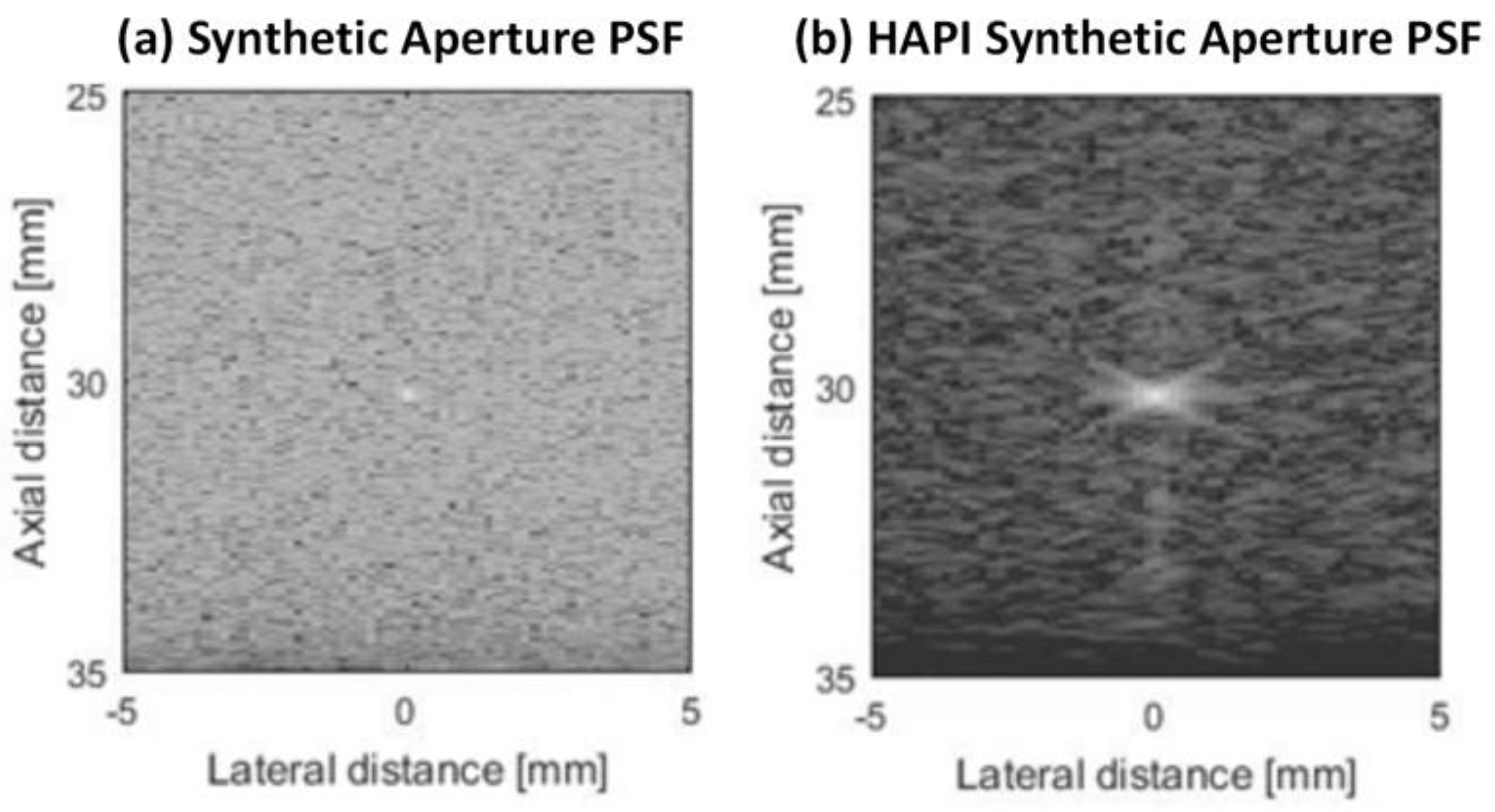
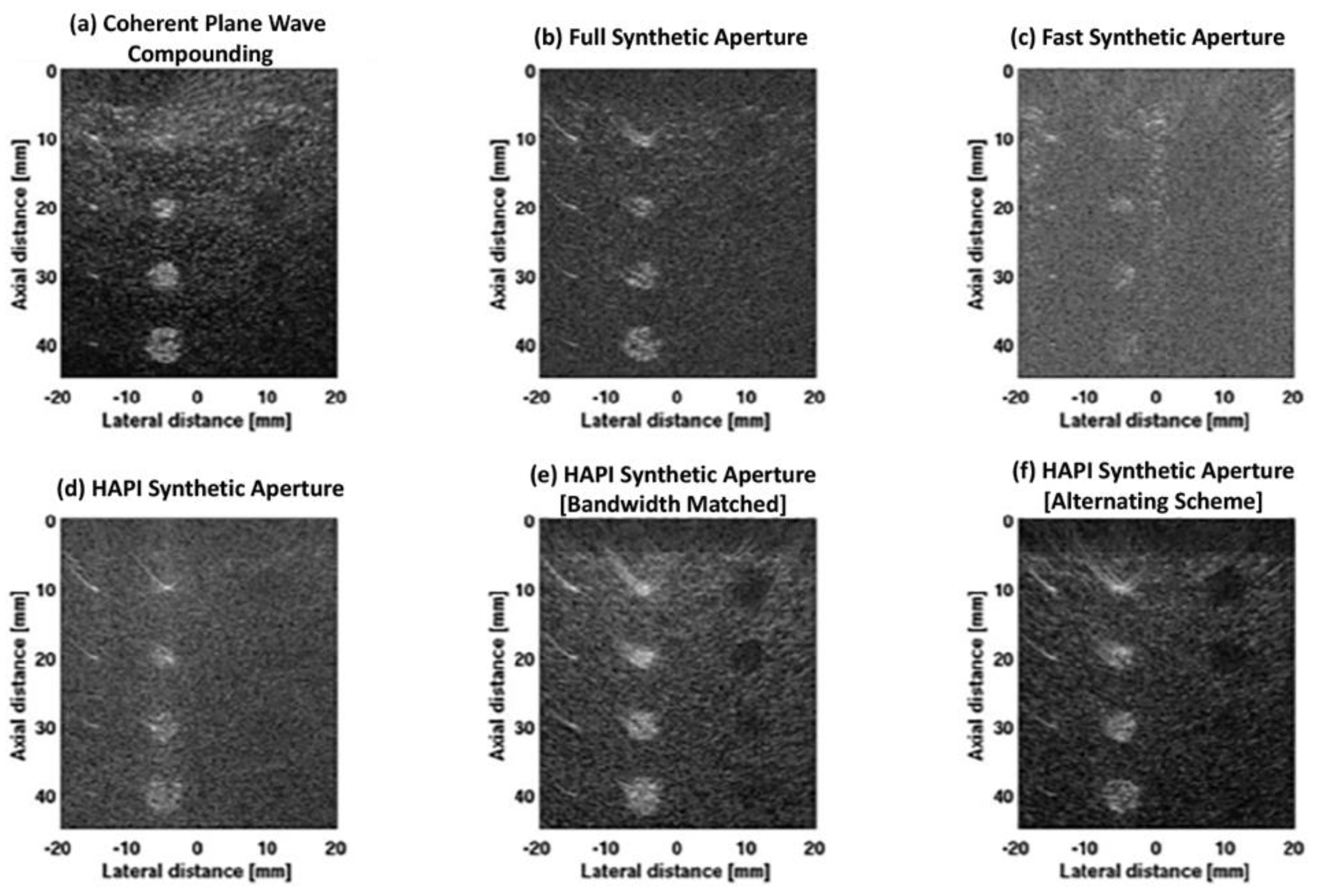
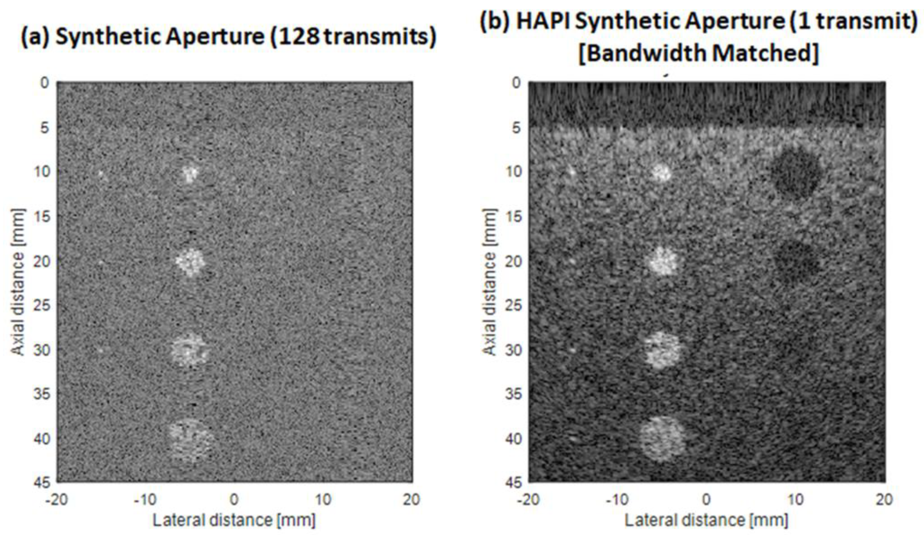
3.1. Linear Array Simulation Results

Figure 4 below compares the point spread functions (PSF) of traditional synthetic aperture (Figure 4a) and bandwidth-matched HAPI synthetic aperture (Figure 4b). It is clear that HAPI-SA produces a less noisy PSF. In fact, the PSF of traditional SA is so noisy at the noise level in this simulation that it is almost impossible to differentiate the single-point scatterer from the noise. The PSF of the SA method appears small because the single-point scatterer is obfuscated by the high amount of noise present in the simulation. The HAPI synthetic aperture PSF is similar in shape and resolution to a noiseless synthetic aperture PSF (data not shown) but exhibits more clutter due to correlation sidelobes.

Figure 5 below compares the simulated images of the scattering phantom for all the imaging methods: (a) coherent plane wave compounding (b) synthetic aperture imaging, (c) fast synthetic aperture imaging, (d) HAPI synthetic aperture imaging without bandwidth matching, (e) HAPI synthetic aperture imaging with bandwidth matching, and (f) HAPI synthetic aperture with the alternating scheme. We can visually see that HAPI-SA imaging with bandwidth matching (Figure 5e) produces the best image in the context of noise. When the bandwidth is not matched (Figure 5d), the image quality suffers. We can also see how the alternating scheme (Figure 5f) of transmitting on every other element, and receiving on the rest, produces an image that is better than traditional synthetic aperture but worse than the full HAPI-SA imaging method that transmits and receives on all elements. This is because only half the synthetic transmit–receive aperture data are obtained in the alternating scheme. The full aperture data can be obtained by imaging with the alternating scheme twice, and switching the elements used for transmit and receive for each transmit event.

Table 2. Comparison of SNR, CNR, and CSR for imaging methods.

	Coherent Plane Wave Compounding		Synthetic Aperture		Synthetic Aperture (3 Sub-apertures of 12 Elements)		HAPI Synthetic Aperture		HAPI Synthetic Aperture (Bandwidth-Matched)		HAPI Synthetic Aperture (Alternating Transmit Scheme)
# Transmit Events	7		128		3		1		1		1
Transmit-Receive Time (ms)	0.41		7.4		0.18		0.6		5.46		5.46
Frame Rate (Hz)	2444		135		5560		1670		183.2		183.2
SNR (dB)	22.33		12.02		10.72		24.87		48.42		36.64
CNR (dB)	HS	Cyst	HS	Cyst	HS	Cyst	HS	Cyst	HS	Cyst	HS	Cyst
10 mm	32.48	7.41	24.01	−5.3	7.52	−20.06	37.96	8.84	69.55	38.93	57.77	27.15
20 mm	33.93	16.28	20.46	−4.24	10.47	−14.03	34.6	11.57	66.34	41.4	54.56	29.62
30 mm	29.22	18.94	19.14	−3.85	7.9	−11.29	30.52	15.57	59.53	42.61	47.75	30.83
40 mm	24.2	19.97	19.14	−2.13	1.3	−14.57	28.47	15.05	56.68	43.74	44.89	31.96
CSR	HS	Cyst	HS	Cyst	HS	Cyst	HS	Cyst	HS	Cyst	HS	Cyst
10 mm	0.55	−0.17	0.92	−0.17	0.63	0.04	0.55	−0.22	1.11	−0.42	1.11	−0.42
20 mm	0.67	−0.6	0.78	−0.19	0.66	−0.08	0.82	−0.31	1.16	−0.57	1.16	−0.57
30 mm	0.7	−0.84	0.66	−0.21	0.56	−0.11	0.7	−0.51	0.98	−0.73	0.98	−0.73
40 mm	0.54	−0.96	0.74	−0.26	0.35	−0.07	0.71	−0.48	0.89	−0.84	0.89	−0.84

below compares the speed, SNR, CNR, and CSR for all of the imaging methods mentioned above. For the CNR and CSR, the five rows of values represent cysts and high scattering (HS) regions at decreasing depths (10 mm, 20 mm, 30 mm, and 40 mm). The SA imaging scheme and bandwidth-matched HAPI-SA are highlighted in the table. Table 2 confirms numerically the visual results from Figure 5. We can see how HAPI-SA with bandwidth matching has the best SNR, CNR, and CSR values compared to all the other imaging methods investigated.

3.2. The 2D Sparse Array Simulation Results

Figure 6 below compares the simulated images of the scattering phantom imaged using a 2D sparse array where active element positions are determined randomly. Images shown are 2D slices in the x-z plane of a 3D volume. Figure 6a shows the image from a synthetic aperture imaging scheme that takes 128 transmits, and Figure 6b shows the image from the encoded HAPI synthetic aperture transmit scheme that takes one extended transmit. We can visually see how HAPI-SA produces the best image in terms of signal-to-noise and contrast-to-noise in much less transmits than synthetic aperture imaging in the context of noise.

4. Discussion

When imaging with a linear array, HAPI synthetic aperture produced a much higher SNR than traditional synthetic aperture or coherent plane wave compounding. Theoretically, there should be a maximum SNR increase of $20{\log }_{10}128=42.14$ dB when comparing 128-element traditional synthetic aperture with HAPI synthetic aperture. The simulation results from Table 2 show that there is a difference in SNR between those two imaging methods of 36.4 dB. This is very close to the theoretical maximum. However, this maximum is only achieved when a Kronecker product is applied to the HAPI code in order to match the bandwidth with the transducer. When this adjustment is not applied, there is only an increase in SNR of 12.85 dB. This result shows the importance of matching the bandwidth so that one can obtain the maximum SNR increase theoretically possible. The difference in SNR and the impact of noise between traditional SA and HAPI-SA can be visually seen in the point spread functions (Figure 4). It is clear that there is much more noise present in traditional SA with 128 transmit events (Figure 4a), compared to HAPI-SA with one transmit event (Figure 4b).

From Figure 5 above, one can visually see how it is easier to differentiate the cysts from the background in the HAPI-SA method compared to traditional SA. At this noise level, it is difficult to locate the cysts with traditional SA (Figure 5b). When we use HAPI-SA imaging without adjusting for the bandwidth of the transducer (Figure 5d), there is only a very small visual increase in contrast compared to SA. However, when the bandwidth is matched (Figure 5e), the contrast increases to the point where it becomes much easier to locate the first three cysts (at 10, 20, and 30 mm) visually. For coherent plane wave compounding (Figure 5a), the cysts are more visible than traditional SA but not as visible as with the bandwidth-matched HAPI-SA method.

These visual results for the cysts are reflected in the CNR calculations in Table 2. HAPI-SA has an average CNR of around 42 dB across the four cyst regions, while traditional SA has an average CNR of −4 dB across the five regions. This makes for a difference of 46 dB. Again, when the bandwidth is not matched, we see a decrease in performance resulting in a difference in average CNR of only 16 dB.

For the high scattering regions in the phantom, it is not as easy to tell the difference in contrast from a visual inspection of the image. Instead, we refer directly to Table 2 to evaluate the performance of the different imaging methods for realizing high scattering regions. Across all imaging methods that were simulated, the CNR of the high scattering regions increases with depth up to a certain point, and then decreases further down. The difference between the average CNR for HAPI-SA compared to traditional SA is 43 dB. Consistent with the previous results, this difference is reduced to 12 dB when the bandwidth is not matched. The CNR of the high scattering regions with coherent plane wave compounding is comparable to the contrast with HAPI-SA without bandwidth matching. With bandwidth matching, the HAPI-SA method has an average CNR that is twice that of coherent plane wave compounding.

The trends for CSR were found to follow the same trends as were discussed for CNR.

Similarly, we see similar trends with the 2D sparse array for 3D imaging. Bandwidth-matched HAPI-SA imaging produced superior images much less susceptible to noise compared to SA imaging. In addition, the HAPI-SA method takes only one extended transmit to form an image, compared to 128 transmits for SA imaging. This shows the potential of HAPI codes to capture 3D volumes with transmit and receive focusing everywhere at hundreds of volumes per second.

From the results it is clear that matching the bandwidth is necessary for achieving maximum performance gains. However, matching the bandwidth results in an increase in code length, which results in an increase in the time to acquire an image. In our case, the code length was increased ten times. Before matching the bandwidth, our code length was 54,415 samples, which translated to a transmit and receive time of 0.54 ms at our sampling frequency of 100 MHz. After matching the bandwidth, the code length is multiplied by 10, and the transmit and receive time is increased to 5.40 ms. This is a significant increase in time, but it is comparable to the amount of time needed to perform 128 transmit events in traditional synthetic aperture. Moreover, our approach achieves a significant SNR advantage, unlike traditional synthetic aperture imaging. For the maximum distance of 45 mm and a speed of sound in soft tissue of 1540 m/s, it would take $128\ast \frac{2\ast 45\mathrm{mm}}{1540\mathrm{m}/\mathrm{s}}$ = 7.5 ms to perform a full synthetic aperture acquisition with 128 elements. Due to the long transmit–receive times of HAPI codes, they are not applicable for fast-moving objects. For example, if we require the imaging target(s) to move less than a tenth of a wavelength over the code duration, this would restrict velocities to below (30 um/5.4 ms = 5.6 mm/s), which may be practical in some static imaging situations, but not applicable to fast-moving tissues. However, the technique may also have applicability to non-destructive testing, underwater acoustics, and air ultrasonics, specifically in cases that do not require detection of fast-moving objects. The codes could additionally be applied to sonar, radar, or communications systems, especially multi-user communications systems that rely on the multiple-input multiple-output paradigm.

The time needed to perform a synthetic aperture image can be reduced by using only a subset of elements to perform a fast synthetic aperture acquisition. If we were to use 3 sub-apertures of 12 elements each, it would only take 0.18 ms to obtain the partial synthetic transmit–receive aperture data. However, using fewer elements will reduce the quality of the image, as seen in Figure 5c. At the noise level in this simulation, it is impossible to obtain a good image with only 3 sub-apertures of 12 elements. This can further be seen in Table 2, where the SNR and CNR have the worst values for fast SA compared to the other imaging methods.

Practical implementation of the codes may require special considerations. Each time a transmit bit is sent it could saturate the amplifiers of the imaging system for tens of nanoseconds to microseconds. The amplifiers will be unable to receive any signals until they recover. This creates a dead zone after each bit is transmitted.

To minimize the dead zone problems or electrical crosstalk during transmission, we introduced the alternating transmit scheme above, where every other element is used for transmit, and the other unused elements for receive. The alternating transmit scheme preserves half the aperture of the array and allows for good imaging quality without sacrificing too much SNR or CNR. If needed, the full SNR and CNR improvement can be realized with the alternating scheme if two transmit events are used. The first transmit event uses every other element to transmit and the other elements to receive, and the second transmit event switches the transmit and receive elements. This way, the full aperture data are collected. However, this approach doubles the transmit time to recover the maximum SNR and CNR gain. Amplifier saturation may not be problematic if transmit amplitudes are sufficiently low and fast amplifier switching is used.

In the case of sparse 2D arrays, it should be easy to implement one sparse pattern of transmitters and a different sparse pattern of elements as receivers. This should also enable extended transmission of codes while allowing for reception during this transmission time without the dead zone problem.

Other coding methods such as those which use Barker and Golay codes do not offer near orthogonal properties of code sets. However, Kasami codes do have near orthogonal properties, and they also meet the Welch lower bound. The Welch bound is the maximum cross-correlation value that can be achieved. For a multi-channel aperiodic correlation, the bound is calculated as Equation (11) [26],

$$c_{max}=\sqrt{\frac{\frac{\mathrm{M}}{\mathrm{K}}-1}{\mathrm{M}\left(2\mathrm{N}-1\right)-1}}$$

(11)

where N is the length of the code, M is the number of codes transmitted in parallel, and K is the number of transmit events.

For our bandwidth-matched 128 non-zero-bit HAPI codes with N = 128, M = 544,150, and K = 1, the maximum bound that can be achieved is $c_{max}$ = 0.00095. However, the actual sidelobe level of the HAPI codes is given by $\frac{1}{\mathrm{M}}$ = 0.0078 for a code length of M = 128. Therefore, HAPI codes do not meet the Welch lower bound, but they do approach it. The small set of Kasami codes, on the other hand, meets the Welch lower bound. However, Kasami codes can become very long if we require them to meet the sidelobe levels of HAPI codes. For a requirement on $c_{max}$ of 42 dB, Kasami codes need to have a code length of 8155 bits. They are also periodic codes, meaning that the transmitter is always on, and they are not sparse and may contain too much energy if appreciable voltage levels are transmitted, potentially violating ultrasound thermal index limits. HAPI codes are also long but they are very sparse, are aperiodic, and thus have minimal energy in them.

Ultrasound systems that can image in real time with synthetic aperture imaging techniques have already been realized. To use HAPI codes on GPU programmable systems, the decoding step needs to be carefully implemented. On receive, decoding is performed by cross-correlating each receive line with each transmit signal to recover the full synthetic aperture dataset. Regular cross-correlation of two vectors involves sliding one vector relative to the other and multiplying the two vectors at each sample. The results are then summed to produce the cross-correlation result. In the case of 128 non-zero-bit bandwidth-matched HAPI codes, this cross-correlation operation would need to be performed for each sample (544,150 samples) and for each transmit–receive combination. This is a significant computational burden. However, because HAPI codes are sparse and they only have 128 non-zero bits, the multiplication stages of the cross-correlation of a single transmit–receive combination need only be performed 128 times for each lag. For a 4.5 cm imaging depth, we require 2400 reconstructed depth samples. At 40 megasamples/second sampling rates and with 256 imaging lines this would require 2.4 GFLOPS to maintain real-time reconstruction rates. This can be performed in real-time using modern computing architectures, some of which are capable of hundreds of TFLOPS.

Few current diagnostic systems may support the transmission of such long codes. However, their generation using custom pulser systems would not be difficult using FPGAs or other programmable devices. Their analysis and computation (beamforming, etc.) would not be difficult to implement in real-time using modern GPUs.

5. Conclusions

We designed a new set of codes called Hadamard Aperiodic Interval codes that are able to produce images with superior SNR with a single extended transmit event. HAPI codes are near orthogonal, so they can be used for parallel transmission in multiple-input multiple-output systems. These codes are also very sparse, as they contain many long intervals of zeros.

Our simulation results show that imaging with the HAPI-SA method produces images with superior signal-to-noise ratio, contrast-to-noise ratio, and contrast-to-speckle ratio compared to traditional SA imaging and coherent plane wave compounding methods. We were able to achieve a maximum SNR increase of 36 dB over traditional SA, close to the predicted maximum from our theoretical calculations.

HAPI codes are among the first codes to be reported which aim to achieve a multiple-input, multiple-output paradigm, where multiple codes are transmitted in parallel with carefully designed auto- and cross-correlation properties. They show promise to improve sensitivity and achieve high contrast-lesion detection capabilities at moderately high frame rates compared to synthetic aperture ultrasound imaging methods. HAPI codes used with sparse 2D arrays show promise for fast 3D volumetric imaging with transmit and receive focusing everywhere throughout the volume.

References

1. Barker, R.H. Group synchronizing of binary digital systems. In Communication Theory; Academic Press: New York, NY, USA, 1953; pp. 273–287. [Google Scholar]
2. Frank, R.L. Polyphase complementary codes. IEEE Trans. Inf. Theory 1980, 26, 641–647. [Google Scholar] [CrossRef]
3. Yan, D.; Ho, P. Acquisition using differentially encoded Barker sequence in DS/SS packet radio. In Proceedings of the IEEE International Conference on Communications ICC ‘95, Seattle, WA, USA, 18–22 June 1995; Volume 3, pp. 1647–1651. [Google Scholar]
4. Bar-David, I.; Krishnamoorthy, R. Barker code position modulation for high rate communication in the ISM bands. In Proceedings of the ISSSTA’95 International Symposium on Spread Spectrum Techniques and Applications, Mainz, Germany, 25–25 September 1996; Volume 3, pp. 1198–1202. [Google Scholar]
5. Latif, S.; Kamran, M.; Masoud, F.; Sohaib, M. Improving DSSS transmission security using Barker code along binary compliments (CBC12-DSSS). In Proceedings of the 2012 International Conference on Emerging Technologies, Islamabad, Pakistan, 8–9 October 2012; pp. 1–5. [Google Scholar]
6. Chiao, R.Y.; Hao, X. Coded excitation for diagnostic ultrasound: A system developer’s perspective. IEEE Trans. Ultrason. Ferroelectr. Freq. Control 2005, 52, 160–170. [Google Scholar] [CrossRef] [PubMed]
7. Friese, M. Polyphase Barker sequences up to length 36. IEEE Trans. Inf. Theory 1996, 42, 1248–1250. [Google Scholar] [CrossRef]
8. Misaridis, T.X.; Pedersen, M.H.; Jensen, J.A. Clinical use and evaluation of coded excitation in B-mode images. In Proceedings of the 2000 IEEE Ultrasonics Symposium, San Juan, PR, USA, 22–25 October 2000; Volume 2, pp. 1689–1693. [Google Scholar]
9. Litniewski, J.; Nowicki, A.; Secomski, W.; Trots, I.; Lewin, P.A. Advantages of probing the trabecular bone with Golay coded ultrasonic excitation. In Proceedings of the IEEE Symposium on Ultrasonics, Honolulu, HI, USA, 5–8 October 2003; Volume 1, pp. 461–464. [Google Scholar]
10. Romero-Laorden, D.; Martinez-Graullera, O.; Martin-Arguedas, C.J.; Parrilla-Romero, M. Application of Golay codes to improve SNR in coarray based synthetic aperture imaging systems. In Proceedings of the 2012 IEEE 7th Sensor Array and Multichannel Signal Processing Workshop, Hoboken, NJ, USA, 17–20 June 2012; pp. 325–328. [Google Scholar]
11. Golay, M.J.E. Complementary series. IEEE Trans. Inf. Theory 1961, 7, 82–87. [Google Scholar] [CrossRef]
12. Nowicki, A.; Litniewski, J.; Secomski, W.; Lewin, P.A.; Trots, I. Estimation of ultrasonic attenuation in a bone using coded excitation. Ultrasonics 2003, 41, 615–621. [Google Scholar] [CrossRef]
13. Hasanudin, H.; Onozato, Y.; Yamamoto, U. A new switching method with orthogonal codes in cellular wireless ATM network. In Proceedings of the 1998 IEEE Asia-Pacific Conference on Circuits and Systems, Chiang Mai, Thailand, 24–27 November 1998; pp. 109–112. [Google Scholar]
14. Ozgur, S.; Williams, D.B. Multi-user detection for mutually orthogonal sequences with space-time coding. In Proceedings of the 2003 IEEE 58th Vehicular Technology Conference, Orlando, FL, USA, 6–9 October 2003; pp. 527–531. [Google Scholar]
15. Poluri, R.; Akansu, A.N. New orthogonal binary user codes for multiuser spread spectrum communications. In Proceedings of the 2005 13th European Signal Processing Conference, Antalya, Turkey, 4–8 September 2005; pp. 1–4. [Google Scholar]
16. DaSilva, V.M.; Sousa, E.S. Multicarrier orthogonal CDMA signals for quasi-synchronous communication systems. IEEE J. Sel. Areas Commun. 1994, 12, 842–852. [Google Scholar] [CrossRef] [Green Version]
17. Pal, M.; Chattopadhyay, S. A novel orthogonal minimum cross-correlation spreading code in CDMA system. In Proceedings of the 2010 International Conference on Emerging Trends in Robotics and Communication Technologies (INTERACT), Chennai, India, 3–5 December 2010; pp. 80–84. [Google Scholar]
18. Gindre, M.; Urbach, W. B-type imaging with coded signals. In Proceedings of the IEEE Ultrasonics Symposium 1993, Baltimore, MD, USA, 31 October–3 November 1993; Volume 2, pp. 1171–1174. [Google Scholar]
19. Gran, F.; Jensen, J.A. Spatial encoding using a code division technique for fast ultrasound imaging. IEEE Trans. Ultrason. Ferroelectri. Freq. Control 2008, 55, 12–23. [Google Scholar] [CrossRef] [PubMed] [Green Version]
20. Garg, G. Low Correlation Sequences for CDMA. In Proceedings of the 2008 IEEE International Networking and Communications Conference, Lahore, Pakistan, 1–3 May 2008; p. 4. [Google Scholar]
21. Boztas, S.; Parampalli, U. Nonbinary sequences with perfect and nearly perfect autocorrelations. In Proceedings of the 2010 IEEE International Symposium on Information Theory, Austin, TX, USA, 13–18 June 2010; pp. 1300–1304. [Google Scholar]
22. Komo, J.J.; Liu, S.-C. Modified Kasami sequences for CDMA. In Proceedings of the Twenty-Second Southeastern Symposium on System Theory, Cookeville, TN, USA, 11–13 March 1990; pp. 219–222. [Google Scholar]
23. Loubet, G.; Capellano, V.; Filipiak, R. Underwater spread-spectrum communications. In Proceedings of the Oceans ‘97. MTS/IEEE Conference, Halifax, NS, Canada, 6–9 October 1997; Volume 1, pp. 574–579. [Google Scholar]
24. Diego, C.; Hernandez, A.; Jimenez, A.; Holm, S.; Aparicio, J. Effect of CDMA techniques with Kasami codes on ultrasound-image quality parameters. In Proceedings of the 2012 IEEE International Instrumentation and Measurement Technology Conference Proceedings, Graz, Austria, 13–16 May 2012; pp. 1833–1837. [Google Scholar]
25. Chandra, A.; Chattopadhyay, S. Small Set Orthogonal Kasami codes for CDMA system. In Proceedings of the 2009 4th International Conference on Computers and Devices for Communication (CODEC), Kolkata, India, 14–16 December 2009; pp. 1–4. [Google Scholar]
26. Welch, L. Lower bounds on the maximum cross correlation of signals (Corresp.). IEEE Trans. Inf. Theory 1974, 20, 397–399. [Google Scholar] [CrossRef]
27. Chiao, R.Y.; Thomas, L.J. Synthetic transmit aperture imaging using orthogonal Golay coded excitation. In Proceedings of the 2000 IEEE Ultrasonics Symposium, San Juan, PR, USA, 22–25 October 2000; Volume 2, pp. 1677–1680. [Google Scholar]
28. Gong, P.; Kolios, M.C.; Xu, Y. Delay-Encoded Transmission and Image Reconstruction Method in Synthetic Transmit Aperture Imaging. IEEE Trans. Ultrason. Ferroelectr. Freq. Control 2015, 62, 1745–1756. [Google Scholar] [CrossRef] [PubMed]
29. Babcock, W.C. Intermodulation interference in radio systems frequency of occurrence and control by channel selection. Bell Syst. Tech. J. 1953, 32, 63–73. [Google Scholar] [CrossRef]
30. Sidon, S. Ein Satz über trigonometrische Polynome und seine Anwendung in der Theorie der Fourier-Reihen. Math. Annalen 1932, 106, 536–539. [Google Scholar] [CrossRef]
31. distributed.net. The OGR-27 Project Has Been Completed. Available online: https://blogs.distributed.net/2014/02/25/16/09/mikereed/ (accessed on 13 April 2022).
32. Jensen, J.A. Field: A Program for Simulating Ultrasound Systems. Med. Biol. Eng. Comput. 1996, 34, 351–353. [Google Scholar]
33. Jensen, J.A.; Svendsen, N.B. Calculation of pressure fields from arbitrarily shaped, apodized, and excited ultrasound transducers. IEEE Trans. Ultrason. Ferroelec. Freq. Control 1992, 39, 262–267. [Google Scholar] [CrossRef] [PubMed] [Green Version]
34. Jensen, J.A.; Nikolov, S.I. Fast simulation of ultrasound images. In Proceedings of the IEEE Symposium (IUS) Ultrasonics, San Juan, PR, USA, 22–25 October 2000; pp. 1721–1724. [Google Scholar]
35. Patterson, M.S.; Foster, F.S. The Improvement and Quantitative Assessment of B-Mode Images Produced by an Annular Array/Cone Hybrid. Ultrason. Imaging 1983, 5, 195–213. [Google Scholar] [CrossRef] [PubMed]
Figure 1. Cross-correlation of v2 and v4 at (a) lag 9, (b) lag 5, (c) lag 1, (d) lag 0, (e) lag −9, and (f) autocorrelation of v2.
Applsci 12 04917 g001
Figure 2. (a) Temporal representation of code v 2 , (b) autocorrelation of code v 2 , (c) cross-correlation of codes v 2 and v 4 , and (d) sum of all the autocorrelations of codes v 1 through v 4 .
Applsci 12 04917 g002
Figure 3. Flow diagram of imaging with HAPI codes. First, 128 HAPI codes are generated. Then they are bandwidth-matched to improve correlation properties. The codes are then transmitted in parallel from all elements and echo signals are received. Decoding is then performed on the echo signals using cross-correlation to recover the full synthetic aperture dataset. Beamforming and summing are then performed on the full recovered dataset to form a high-resolution image.
Applsci 12 04917 g003
Figure 4. Point spread functions of (a) traditional synthetic aperture with 128 elements (128 transmit events), and (b) HAPI synthetic aperture with 128 non-zero-bit codes (1 transmit event) and bandwidth matching. For the same amount of noise added to the scattering data, HAPI-SA produces less noise in the resultant image. Images have a 55 dB dynamic range.
Applsci 12 04917 g004
Figure 5. Simulation images of the phantom with 4 hypoechoic cysts and 4 high scattering regions placed at decreasing depths (10 mm, 20 mm, 30 mm, 40 mm) for (a) coherent plane wave compounding with 7 angles equally spaced between −18° and 18°, (b) traditional synthetic aperture imaging with 128 transmit events, (c) fast synthetic aperture imaging with 3 sub-apertures, (d) HAPI synthetic aperture imaging with 1 transmit event but no bandwidth matching, (e) HAPI synthetic aperture imaging with bandwidth matching, and (f) HAPI synthetic aperture imaging with an alternating transmit scheme. HAPI-SA with bandwidth matching (e) produces the best images of all the above. The alternating transmit scheme (f) of transmitting on every other element and receiving on the rest produces an image better than traditional SA (a) but worse than the full HAPI-SA (e). When the bandwidth is not matched, the quality of the image suffers (d). All images are shown at a 55 dB dynamic range.
Applsci 12 04917 g005
Figure 6. The 2D sparse array simulation images of the phantom with 4 hypoechoic cysts and 4 high scattering regions placed at decreasing depths (10 mm, 20 mm, 30 mm, 40 mm) for (a) synthetic aperture imaging using 128 transmits, and (b) Hadamard Aperiodic Interval synthetic aperture imaging using 1 transmit. Images are 2D slices of the x-z plane of a 3D volume displayed at −55 dB.
Applsci 12 04917 g006