
Damage Detection and Level Classification of Roof Damage after Typhoon Faxai Based on Aerial Photos and Deep Learning


Abstract
:1. Introduction
1.1. Purpose and Significance
1.2. Previous Research
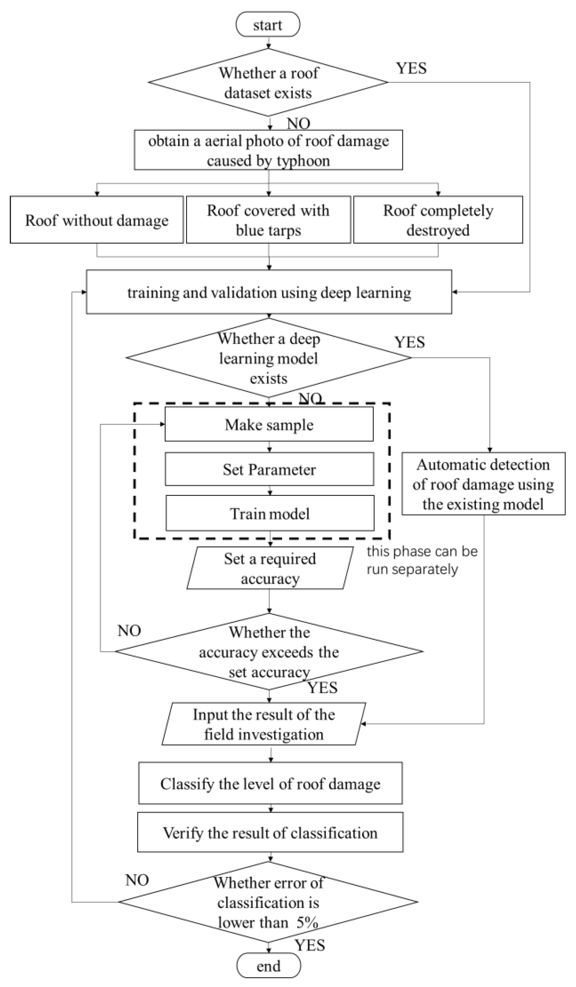
2. Research Methods
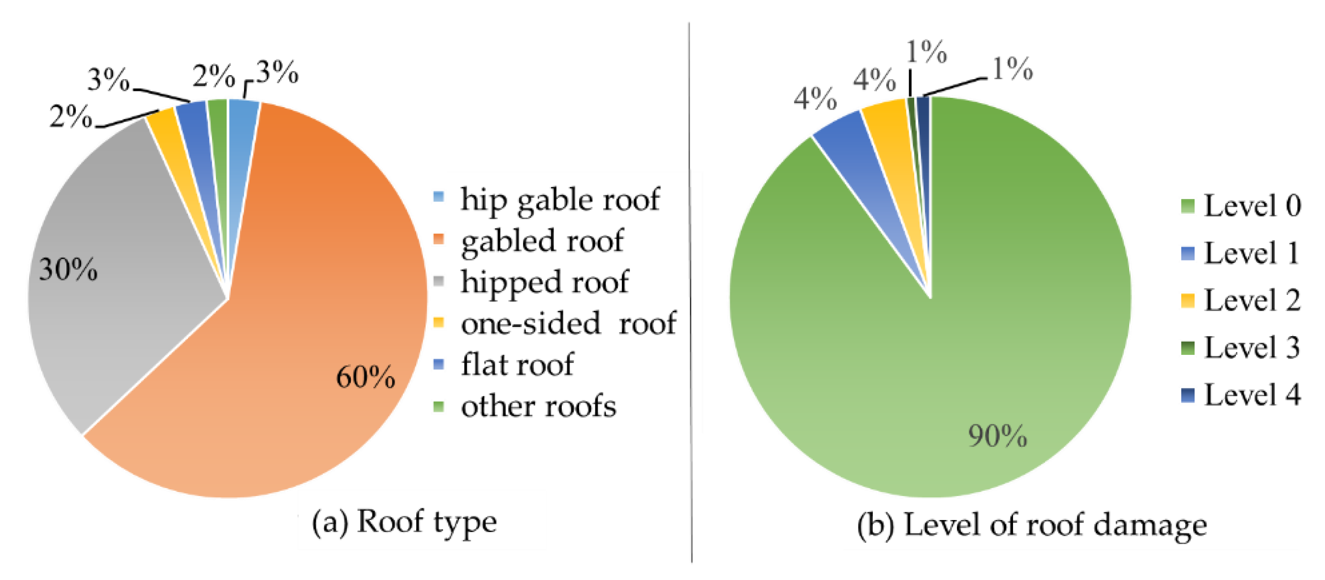
3. Materials
3.1. Used Aerial Photos
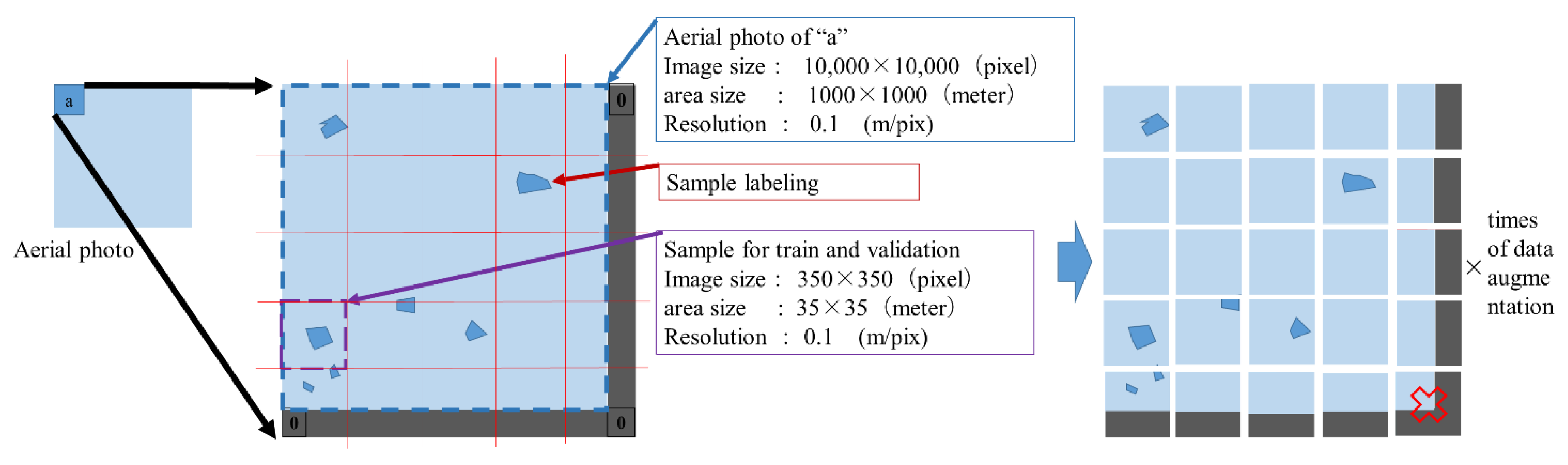
3.2. Labeling and Cropping Aerial Photos
3.3. Export Data
4. Training and Detection Using Deep Learning
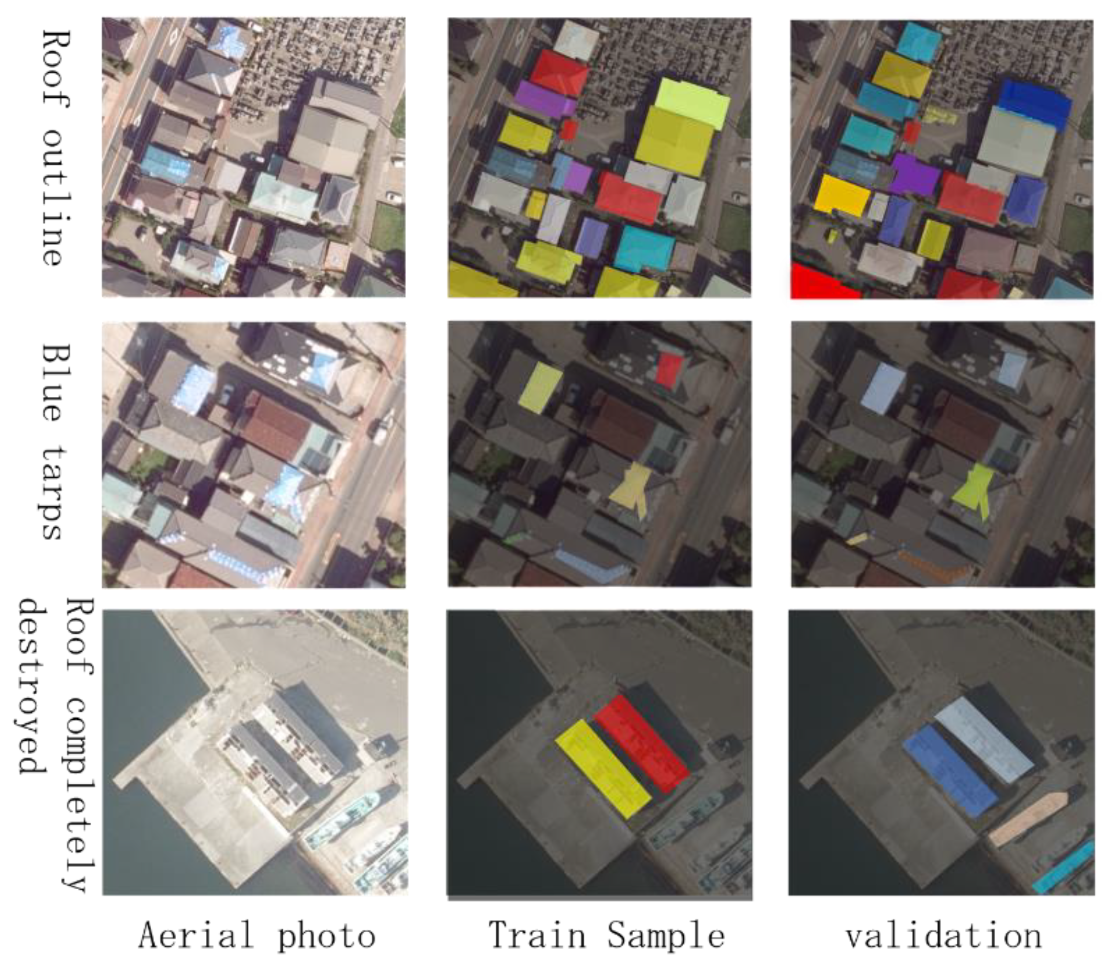
4.1. Making Sample
4.2. Setting Parameters
4.3. Training Model
4.3.1. Loss Function in Training
4.3.2. Optimization Algorithm
4.3.3. Training Process
4.4. Validation in Training
4.5. Test after Training
4.6. Comparison with Field Investigation
5. Classification of Roof Damage Level
6. Discussion
7. Conclusions
Author Contributions
Funding
Institutional Review Board Statement
Informed Consent Statement
Data Availability Statement
Acknowledgments
Conflicts of Interest
References
- National Institute for Land and Infrastructure Management (NILIM); Building Research Institute (BRI). Disaster report: Field Survey report on damage to buildings due to strong winds caused by typhoon Faxai in 2019 (Summary). Build. Disaster Prev. 2019, 503, 57–66. [Google Scholar]
- National Institute for Land and Infrastructure Management (NILIM). Field Investigation Report on Damage of Buildings by Strong Wind Accompanied with Typhoon No.21. Available online: http://www.nilim.go.jp/lab/bbg/saigai/ (accessed on 14 November 2018).
- Cabinet Office (Disaster Prevention): Disaster Guidelines for Disaster Victims 2021. Available online: http://www.bousai.go.jp/taisaku//pdf/r303shishin_all.pdf (accessed on 18 March 2021).
- Kazuyoshi, N.; Yuya, K.; Takashi, T.; Eriko, T.; Hiroshi, N. Survey report on damage and recovery after Typhoon Faxai in 2019: Part1-Part4. Analysis of roof damage with aerial photo image. In Summaries of Technical Papers of Annual Meeting, Architectural Institute of Japan; Chiba University: Chiba, Japan, 2020; pp. 46–85. [Google Scholar]
- Ministry of Internal Affairs and Communications, Japan. Result Report: Fact-Finding Survey on the Issuance of Disaster Certificates in the Event of a Large-Scale Disaster, Focusing on the 2016 Kumamoto Earthquakes. Available online: https://www.soumu.go.jp/main_content/000528758.pdf (accessed on 18 March 2021).
- Mitomi, H.; Matsuoka, M.; Yamazaki, F.; Taniguchi, H.; Ogawa, Y. Determination of the areas with building damage due to the 1995 Kobe earthquake using airborne MSS images. IEEE Int. Geosci. Remote Sens. Symp. 2002, 5, 2871–2873. [Google Scholar]
- Noda, M.; Tomokiyo, E.; Takeuchi, T. Aerial survey of wind damage by T1821 in South Osaka and North Wakayama. Summ. Tech. Pap. Annu. Meet. Jpn. Assoc. Wind. Eng. 2019, 1, 105–106. [Google Scholar]
- Suzuki, K.; Hanada, D.; Yamazaki, F. building damage inspection of the 2012 Tsukuba Tornado from field survey and aerial photographs. Inst. Soc. Saf. Sci. 2013, 21, 9–16. [Google Scholar]
- Kono, Y.; Kazuyoshi, N.; Takashi, T.; Eriko, T.; Hiroshi, N. Housing damage caused by Typhoon Jebi 2018 Part 1 Estimation of roof damage rate based on comparison of satellite images taken before and after the typhoon. Archit. Inst. Jpn. 2020, 1, 72–85. [Google Scholar]
- Kono, Y.; Nishijima, K. Survey report on damage and recovery after Typhoon Faxai in 2019: Part4: Analysis of roof damage with aerial photo image. Archit. Inst. Jpn. 2019, 2, 89–99. [Google Scholar]
- Naito, S.; Monma, N.; Yamada, T.; Shimomura, H.; Mochizuki, K.; Honda, Y.; Nakamura, H.; Fujiwara, H.; Shoji, G. Building damage detection of the kumamoto earthquake utilizing image analyzing methods with aerial photographs. J. Jpn. Soc. Civ. Eng. 2019, 75, 218–237. [Google Scholar] [CrossRef]
- Kurihara, S. The Theory of the Future of Life, Industry and Society from the Viewpoint of the Practical Use of AI Revolution with Human Being; NTS Press: Tokyo, Japan, 2019; pp. 49–113. (In Japanese) [Google Scholar]
- Hiroyuki, M.; Aridome, T.; Matsuoka, M. Deep learning-based identification of collapsed, non-collapsed and blue tarp-covered buildings from post-disaster aerial photo. Remote Sens. 2020, 12, 1924. [Google Scholar]
- Minshui, H.; Wei, Z.; Jianfeng, G.; Yongzhi, L. Damage identification of a steel frame based on integration of time series and neural network under varying temperatures. Adv. Civ. Eng. 2020, 1, 1–15. [Google Scholar]
- Ministry of Internal Affairs and Communications, Japan: About the Damage Situation Caused by Typhoon Faxai in 2019. Available online: https://www.soumu.go.jp/r01_taifudai15gokanrenjoho/ (accessed on 18 March 2021).
- Hinz, A. The Z/I Imaging digital aerial camera system. In Photogrammetric Week 1999; Fritsch, D., Spiller, R., Eds.; Wichmann Verlag: Heidelberg, Germany, 1999. [Google Scholar]
- Kaiming, H.; Gkioxari, G.; Dollar, P.; Girshick, R. Mask R-CNN. In Proceedings of the IEEE International Conference on Computer Vision, Venice, Italy, 22–29 October 2017; pp. 2961–2969. [Google Scholar]
- Girshick, R.; Donahue, J.; Darrell, T.; Malik, J. Region-based convolutional networks for accurate object detection and segmentation. IEEE Trans. Pattern Anal. Mach. Intell. 2016, 38, 142–158. [Google Scholar] [CrossRef] [PubMed]
- Lin, T.Y.; Dollár, P.; Girshick, R.; He, K.; Hariharan, B.; Belongie, S. Feature pyramid networks for object detection. In Proceedings of the IEEE Conference on Computer Vision and Pattern Recognition, Honolulu, HI, USA, 21–26 July 2017; pp. 936–944. [Google Scholar]
- Ross, R. Fast R-CNN. In Proceedings of the IEEE International Conference on Computer Vision, Santiago, Chile, 7–13 December 2015; pp. 1440–1448. [Google Scholar]
- Ren, S.; He, K.; Girshick, R.; Sun, J. Faster R-CNN: Towards real-time object detection with region proposal networks. IEEE Trans Pattern Anal. Mach. Intell. 2016, 39, 1137–1149. [Google Scholar] [CrossRef] [PubMed] [Green Version]
- Paszke, A.; Gross, S.; Massa, F.; Lerer, A.; Bradbury, J.; Chanan, G.; Killeen, T.; Lin, Z.; Gimelshein, N.; Antiga, L.; et al. PyTorch, an imperative style, high-performance deep learning library. Adv. Neural Inf. Process. Syst. 2019, 32, 8026–8037. [Google Scholar]
- Lin, T.Y.; Maire, M.; Belongie, S.; Hays, J.; Perona, P.; Ramanan, D.; Dollár, P.; Zitnick, C.L. Microsoft COCO: Common objects in context. In Computer Vision—ECCV 2014. ECCV 2014; Lecture Notes in Computer Science; Fleet, D., Pajdla, T., Schiele, B., Tuytelaars, T., Eds.; Springer: Cham, Switzerland, 2014; pp. 740–755. [Google Scholar]
- Minshui, H.; Cheng, X.; Zhu, Z.; Luo, J.; Gu, J. A novel two-stage structural damage identification method based on superposition of modal flexibility curvature and whale optimization algorithm. Int. J. Struct. Stab. Dyn. 2021, 21, 2150169. [Google Scholar]
- Minshui, H.; Cheng, X.; Lei, Y. Structural damage identification based on substructure method and improved whale optimization algorithm. J. Civ. Struct. Health Monit. 2021, 11, 351–380. [Google Scholar]
- Chida, H.; Takahashi, N. Study on image diagnosis of timber houses damaged by earthquake using deep learning. Archit. Inst. Jpn. J. Struct. Constr. Eng. 2020, 85, 529–538. [Google Scholar] [CrossRef]
- Garcia-Garcia, A.; Orts-Escolano, S.; Oprea, S.; Villena-Martinez, V.; Garcia-Rodriguez, J. A review on deep learning techniques applied to semantic segmentation. arXiv 2017, arXiv:1704.06857. [Google Scholar]
- Kanai, K.; Yamane, T.; Ishiguro, S.; Chun, P.-J. Automatic detection of slope failure regions using semantic segmentation. Intell. Inform. Infra. 2020, 1, 421–428. [Google Scholar]
- Statistics Bureau of Japan. About Regional Mesh Statistics. Available online: https://www.stat.go.jp/data/mesh (accessed on 24 December 2020).
- Liu, W.; Maruyama, Y. Damage estimation of buildings’ roofs due to the 2019 typhoon Faxai using the post-event aerial photographs. J. Jpn. Soc. Civ. Eng. 2020, 76, 166–176. [Google Scholar] [CrossRef]


| Investigation | Total | Percentage |
|---|---|---|
| Surveyed houses | 1976 | - |
| Damaged house | 1133 | 57% |
| Damaged Roof | 902 | 46% |
| Damaged Wall | 228 | 12% |
| Number of Labeling | Roof Outline | Blue Tarps | Roof Completely Destroyed | Total |
|---|---|---|---|---|
| Labeling at area T1–T18 | 21,600 | 3221 | 384 | 25,205 |
| Labeling at area K1–K5 | 2697 | 506 | 66 | 3269 |
| Labeling at all area | 24,297 | 3727 | 450 | 28,474 |
| Parameters | Set A | Set B | Set C | Set D |
|---|---|---|---|---|
| Batch size (note1) | 8 | 16 | 32 | 64 |
| Ratio of training and validation | 10% | 10% | 20% | 20% |
| Backbone (note2) | Resnet 50 | Resnet 50 | Resnet 101 | Resnet 101 |
| Train time for evaluation | 6000 | 6000 | 6000 | 6000 |
| Initial learning rate (note3) | 1 × 10⁻² | 1 × 10⁻⁴ | 1 × 10⁻³ | 5 × 10⁻⁵ |
| Detected Object | TP | FN | FP | TN |
|---|---|---|---|---|
| Roof outline | 10,312,006 | 1,274,517 | 1,390,382 | 87,023,095 |
| Blue tarps | 257,733 | 22,909 | 28,637 | 99,690,721 |
| Roofs completely destroyed | 213,646 | 60,259 | 21,912 | 99,704,183 |
| Detected Object | Accuracy | Precision | Recall | Specificity | F Value |
|---|---|---|---|---|---|
| Root outline | 0.973 | 0.881 | 0.890 | 0.984 | 0.886 |
| Blue tarps | 0.999 | 0.900 | 0.918 | 0.999 | 0.909 |
| Roofs completely destroyed | 0.999 | 0.907 | 0.780 | 0.999 | 0.839 |
| (a) | |||||||
| Classification Using Visual Inspection | Classification Using Deep Learning | ||||||
| Level 4 | Level 3 | Level 2 | Level 1 | Level 0 | Non-Object | Total | |
| Level 4 | 82 | 0 | 0 | 0 | 13 | 8 | 103 |
| Level 3 | 2 | 39 | 7 | 5 | 4 | 5 | 62 |
| Level 2 | 1 | 8 | 247 | 32 | 5 | 25 | 318 |
| Level 1 | 3 | 5 | 29 | 299 | 14 | 25 | 375 |
| Level 0 | 6 | 0 | 2 | 8 | 7112 | 521 | 7649 |
| non-object | 6 | 0 | 0 | 2 | 154 | 6 | 168 |
| total | 100 | 52 | 285 | 346 | 7302 | 590 | 8675 |
| (b) | |||||||
| level of Classification | Accuracy | Precision | Recall | Specificity | F Value | ||
| Level 4 | 0.996 | 0.820 | 0.796 | 0.815 | 0.808 | ||
| Level 3 | 0.996 | 0.750 | 0.629 | 0.994 | 0.684 | ||
| Level 2 | 0.987 | 0.867 | 0.777 | 0.995 | 0.819 | ||
| Level 1 | 0.986 | 0.864 | 0.797 | 0.998 | 0.829 | ||
| Level 0 | 0.916 | 0.974 | 0.930 | 0.998 | 0.951 | ||
| average value | 0.976 | 0.855 | 0.786 | 0.960 | 0.818 | ||
| Compared Article | Method of Classification | Number of Parts | Parts of Classification | Accuracy | Average Accuracy | F Value | Average F Value |
|---|---|---|---|---|---|---|---|
| Noda et al. [7] | visual inspection | 2 parts | roof without blue tarps | 1.000 | 1.000 | 1.000 | 1.000 |
| roof covered with blue tarps | 1.000 | 1.000 | |||||
| Kono et al. [10] | image analysis | 2 parts | roof without blue tarps | 0.746 | 0.800 | 0.738 | 0.791 |
| roof covered with blue tarps | 0.929 | 0.844 | |||||
| Liu et al. [30] | image analysis | 3 parts | roof without blue tarps | 0.920 | 0.880 | 0.935 | 0.801 |
| roof partially covered with blue tarps | 0.810 | 0.791 | |||||
| roof mostly covered with blue tarps | 0.720 | 0.677 | |||||
| Miura et al. [13] | Deep learning (CNN) | 3 parts | roof without damage | 0.926 | 0.937 | 0.955 | 0.730 |
| roof with blue tarps | 0.964 | 0.944 | |||||
| roof completely destroyed | 0.833 | 0.291 | |||||
| this paper | Deep learning (Mask R-CNN) | 5 parts | roof without damage | 0.916 | 0.976 | 0.951 | 0.818 |
| roof covered with 0–10% blue tarps | 0.986 | 0.829 | |||||
| roof covered with 10–50% blue tarps | 0.987 | 0.819 | |||||
| roof covered with 50–100% blue tarps | 0.996 | 0.684 | |||||
| roof completely destroyed | 0.996 | 0.808 |
Publisher’s Note: MDPI stays neutral with regard to jurisdictional claims in published maps and institutional affiliations. |
© 2022 by the authors. Licensee MDPI, Basel, Switzerland. This article is an open access article distributed under the terms and conditions of the Creative Commons Attribution (CC BY) license (https://creativecommons.org/licenses/by/4.0/).
Share and Cite
Xu, J.; Zeng, F.; Liu, W.; Takahashi, T. Damage Detection and Level Classification of Roof Damage after Typhoon Faxai Based on Aerial Photos and Deep Learning. Appl. Sci. 2022, 12, 4912. https://doi.org/10.3390/app12104912
Xu J, Zeng F, Liu W, Takahashi T. Damage Detection and Level Classification of Roof Damage after Typhoon Faxai Based on Aerial Photos and Deep Learning. Applied Sciences. 2022; 12(10):4912. https://doi.org/10.3390/app12104912
Chicago/Turabian StyleXu, Jinglin, Feng Zeng, Wen Liu, and Toru Takahashi. 2022. "Damage Detection and Level Classification of Roof Damage after Typhoon Faxai Based on Aerial Photos and Deep Learning" Applied Sciences 12, no. 10: 4912. https://doi.org/10.3390/app12104912
APA StyleXu, J., Zeng, F., Liu, W., & Takahashi, T. (2022). Damage Detection and Level Classification of Roof Damage after Typhoon Faxai Based on Aerial Photos and Deep Learning. Applied Sciences, 12(10), 4912. https://doi.org/10.3390/app12104912