A Phase Correlation Anti-Noise Displacement Estimation Method Based on PSD Phase Screening

Abstract

When using digital images to obtain the displacement of a structure, noise is always a factor that greatly affects the accuracy of the displacement results. To overcome this problem, a phase-correlation improvement method, based on phase filtering by phase standard deviation (PSD), is proposed. We use PSD to remove the severe noise interference area in the cross-power spectrum matrix, then the singular value decomposition (SVD) is used to convert the two-dimensional phase to one-dimensional to reduce the difficulty of phase unwrapping. Finally, straight-line fitting is used to obtain the high-precision displacement results. Experiments were carried out using both simulated data and real data. For the simulated data, the absolute accuracy of the proposed method is around 0.3 pixels, while, for the real data, the absolute accuracy of the proposed method is 0.018 mm. The experimental results show that the method can effectively resist noise interference and still obtain accurate displacement estimation results in the case of severe noise.

1. Introduction

With the rapid development of the world economy, the demand for transportation is increasing. Therefore, at the beginning of this century, China and other countries has been vigorously building high-speed railways [1,2], and more high-speed railway lines and rail bridges have been constructed. With the extension of operation time, various problems may occur that result in safety problems. The manpower losses and financial losses caused by the damage of railroad tracks and bridges are immeasurable. Therefore, it is necessary to monitor the health condition of these rails and bridges.

Various methods have been proposed to monitor the health of rails and bridges; the first kind of method is based on traditional equipment such as a displacement meter, total station, and level instrument; the second kind of method is based on new technology such as Global Navigation Satellite System (GNSS) technology [3,4], Interferometric Synthetic Aperture Radar (InSAR) technology [5,6] and Light Detection and Ranging (Lidar) technology [7,8]; and the third kind of method is based on visual monitoring [9,10]. Methods based on traditional equipment can demonstrate the best precision, but are unable to monitor automatically; those methods based on newly developed technology can realize automatic monitoring, but the costs are expensive. Thanks to the rapid development of industrial cameras with high temporal and spatial resolution, the cost of visual monitoring has decreased. In addition, this technology is rapidly developing, as more scholars have invested in the research of visual monitoring technology during recent years. For example, Barkhordari et al. [11] used visual-based methods for automatic structural damage identification; Wang et al. [12] proposed a lightweight measurement method based on smartphone images and developed corresponding mobile phone software for this method; Alessandro Galdelli et al. [13] designed a new remote visual inspection system for bridge predictive maintenance based on a visual-based monitoring method.

Using the visual-based method to monitor the deformation of tracks and bridges, the general process is as follows: a camera is used to continuously capture images for the monitoring object, and then the frame and inter-frame displacement information (pixel unit) is obtained according to the image, then the corresponding scale of the image (the real size corresponding to each pixel) is calculated, and, finally, the physical displacement is calculated according to the real scale. There are two commonly used ways to obtain frame and frame displacement. (1) Pasting targets or speckle patterns on bridges and capturing the displacement sequences of rails and bridges by shooting and tracking the targets or speckle patterns [14]; this method needs to paste the targets or digital speckles on the monitoring objects, which may not be applicable in some situations. (2) Depending on the characteristics of bridges and rails, a digital image correlation is used to obtain the target displacement sequence [15,16,17]. In the high-frequency vibration monitoring of tracks and bridges, due to the high shooting frequency of the camera and the long shooting distance [18], the image quality is not ideal, which makes it difficult to directly track the target on the grayscale image. Therefore, the phase correlation method, which is more noise-resistant, is a better choice.

Research into the phase correlation algorithm has a long history. The algorithm uses a Fourier transform to transfer digital image from a space domain to a frequency domain, and then correlation operations are performed on the two images in the frequency domain to obtain the displacement between the two images [19,20]. In 1975, Kuglin and Hines [21] first proposed a digital image phase correlation algorithm and applied it to image registration. Compared with digital image grayscale correlation, it has a certain anti-noise performance and has a certain degree of anti-noise performance. It has advantages such as insensitivity [22], so it is widely used to calculate the displacement between images [23,24,25,26]. The most primitive phase correlation method can only obtain pixel-level displacement. So, there were several scholars working to improve the performance of phase correlation, who proposed phase line fitting [27,28,29], phase plane fitting [30,31,32], tooth signal number estimation [33,34], frequency estimation [35], local up-sampling [36], and other optimization methods [37,38,39] to enable the phase correlation method to obtain subpixel precision displacement.

Although the phase correlation method has better anti-noise performance than the grayscale correlation method, the signal-to-noise ratio would be extremely low in images captured in some scenes, such as high-frequency shooting, insufficient ambient light, etc. In order to further improve the anti-noise performance of phase correlation, some scholars have proposed the use of the SVD decomposition method [40,41] or the random sampling consistency method (RANSAC) [42,43] to further solve the noise problem in phase correlation displacement estimation. These methods are indeed helpful for further improving the anti-noise performance of phase correlation, but there are still some limitations. For example, when the proportion of the noise is much larger than the proportion of the true phase, SVD decomposition cannot accurately restore the true phase; in addition, the RANSAC method may not work when noise interference is particularly severe.

In general, the existing phase correlation methods can achieve higher accuracy when the noise is not particularly severe. However, when the noise interference is particularly severe, the accuracy will decrease to a certain extent. Aiming at the situation of particularly severe noise, this paper proposes a phase correlation improvement method based on PSD [44] phase screening, to accurately estimate the displacement of the scene under severe noise conditions. Firstly, PSD is used to remove the cross-power spectrum matrix area that is severely disturbed by noise, then SVD is used to convert the phase into one dimension, which reduces the difficulty of phase unwrapping, and, finally, a least squares straight-line fitting method is used to obtain the displacement of the subject scene.

The remainder of this paper is organized as follows. Section 2 describes the specific approach of the method in this paper, the experimental validation part of this paper is discussed Section 3, including simulated data experiments and real data validation experiments, and the conclusions and future work are in Section 4.

2. Methods

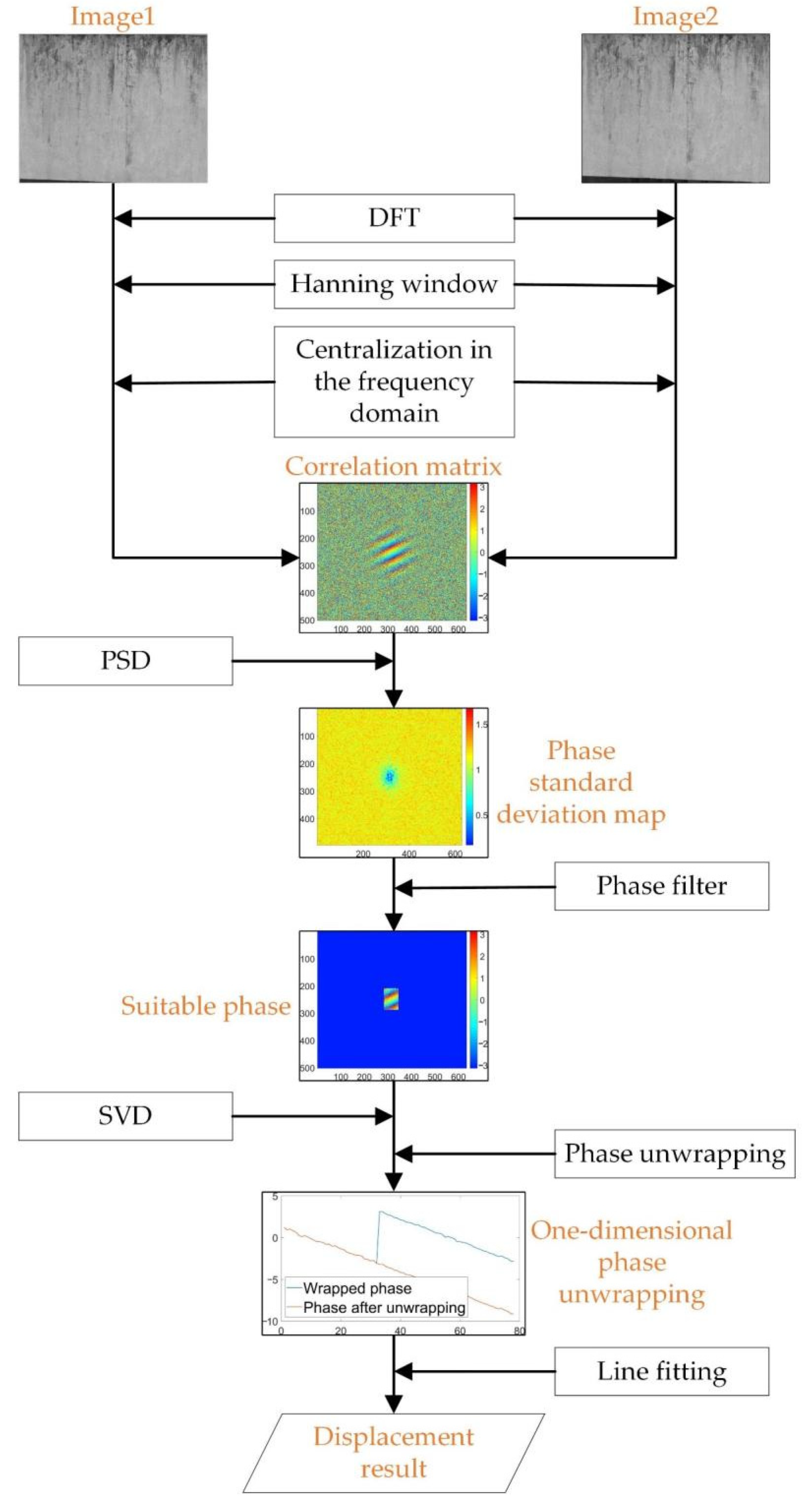
Based on the traditional phase correlation, this paper introduced the PSD to evaluate the clarity of the cross-power spectrum matrix interference fringe, and prescreens the cross-power spectrum matrix according to the evaluation results, so as to automatically remove the areas with severe disturbances from the cross-power spectrum matrix. The workflow of the proposed method is shown in Figure 1.

The input of the workflow is sequence images that show possible displacement between nearby continuing images. Firstly, the two-dimensional discrete Fourier transform (DFT) is used to convert the two images before (image 1 in Figure 1) and after displacement (image 2 in Figure 1) to the frequency domain. To prevent spectral leakage, the two images were windowed after converting to the frequency domain. In addition, in order to concentrate the areas that are not disturbed by noise, we performed frequency domain centering on the two frequency domain images, and then the two frequency domain images are interfered with to obtain the cross-power spectrum matrix. Secondly, the PSD of the cross-power spectrum matrix is calculated to screen out the clear area of the cross-power spectrum matrix. Then, SVD is used to convert the cross-power spectrum matrix to one dimension, and one-dimensional phase unwrapping is performed. Finally, the displacement is solved by fitting a straight line based on the unwrapping phase. The details are explained as follows.

2.1. Cross-Power Spectrum Matrix Acquisition

According to the classical phase correlation principle, an image $f_2\left(x, y\right)$ is the image obtained by translating image $f_1\left(x, y\right)$ with $\left(x_0, y_0\right)$, that is, $f_2\left(x, y\right)=f_1\left(x-y_0, y-y_0\right)$. Let $F_1\left(u, v\right), F_2\left(u, v\right)$ be the two-dimensional DFT results of $f_1\left(x, y\right)$, $f_2\left(x, y\right),$ respectively, and then, according to the Fourier time-shift properties, we can get:

$$F_2\left(u,v\right)=F_1\left(u,v\right)\times e^{-i\left(u{x}_0+v{y}_0\right)}$$

(1)

Divide the left side of Equation (1) by the right side to get the cross-power spectrum matrix $Q\left(u,v\right),$ per Equation (2):

$$Q\left(u,v\right)=\frac{F_1\left(u,v\right)F_2{}^{*}\left(u,v\right)}{\left|F_1(u,v)F_2{}^{*}(u,v)\right|}=e^{-i\left(u{x}_0+v{y}_0\right)}$$

(2)

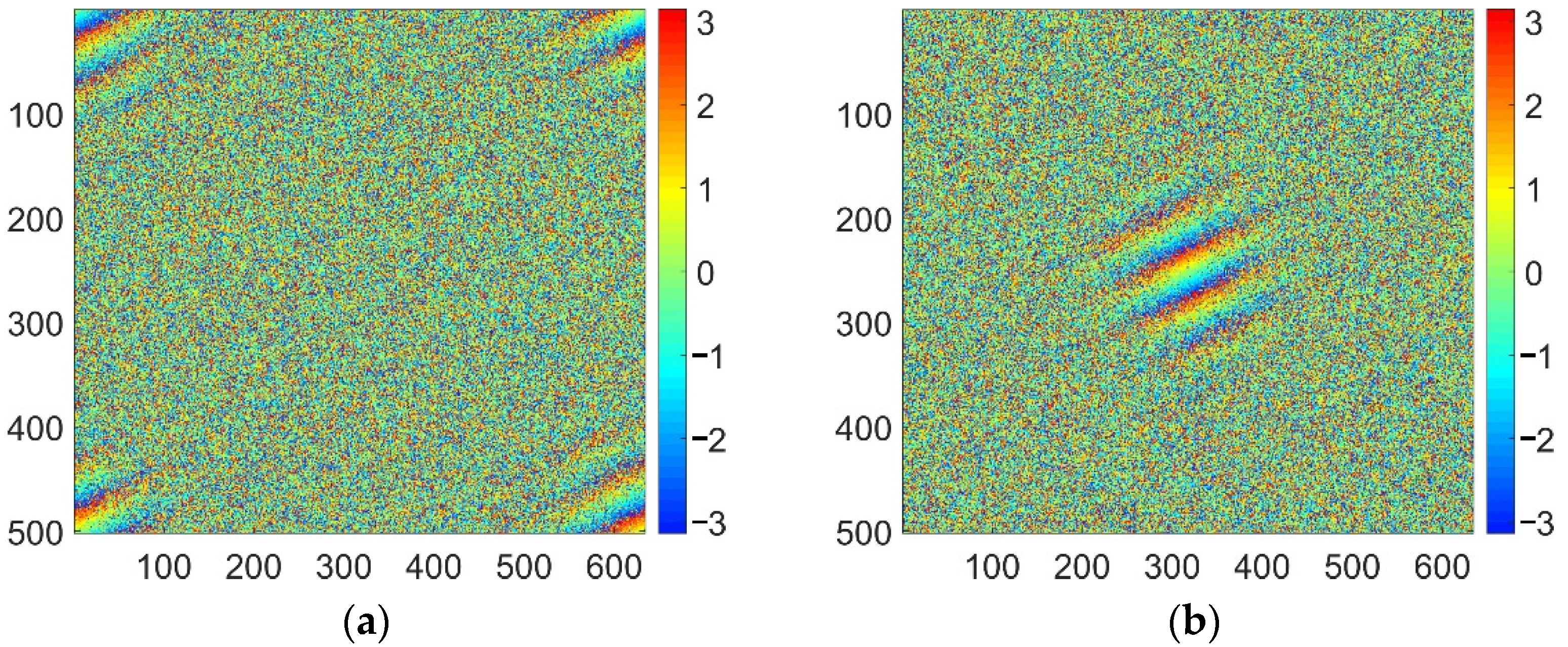
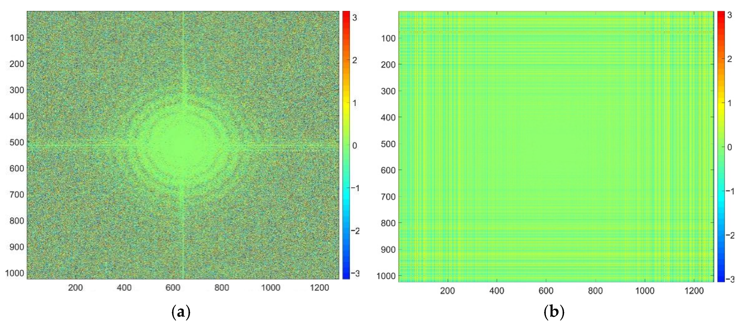
Since the low-frequency part of the cross-power spectrum matrix obtained in Equation (2) is in the upper-left corner of the matrix, frequency domain centering is needed in the actual processing process, so that the low-frequency part of the cross-power spectrum matrix is in the center, while the high-frequency part is around it. As shown in Figure 2, Figure 2a represents the cross-power spectrum matrix’s phase without frequency domain centering, and Figure 2b represents the cross-power spectrum matrix’s phase, where the frequency domain is centralized. It clearly demonstrates that after performing the frequency domain centralization, the areas with clear fringes can be gathered together, which is convenient for subsequent processing.

In addition, the two-dimensional DFT assumes that the input signal is an infinitely long period signal. However, the image actually does not meet this requirement, which will cause the problem of spectrum leakage in the actual processing. Therefore, windowing is required after the Fourier transformation. In this paper, the Hanning window function is used for windowing [45]. The function is defined per Equation (3):

$$W_k\left(u,v\right)=\frac{1}{4}\left[1+\cos \left(\frac{u-H/2}{H}\pi \right)\right]\left[1+\cos \left(\frac{v-W/2}{W}\pi \right)\right]$$

(3)

where $W$ is the width of the image, $H$ is the height of the image.

2.2. PSD-Based Phase Screening

The cross-power spectrum matrix obtained in the previous section is a complex matrix with a phase that is a periodic toothed fringe signal. The displacement between the two images can be estimated based on the toothed fringe signal. The fringe is clear under ideal conditions, but there will be a lot of speckle noise in the fringe due to the presence of noise during image acquisition. In some extreme cases, the fringe is not visible at all, which makes it is uncertain to estimate the displacement.

In view of the serious noise interference of the cross-power spectrum matrix, this paper utilizes PSD to evaluate the clarity of the phase fringes and then screen out the cross-power spectrum matrix regions with clear fringes, based on the evaluation results. According to the definition of PSD [40], to calculate every element in the phase of the cross-power spectrum matrix, a neighboring window with $\mathrm{w}\times \mathrm{w}$ has to be considered, per Equation (4). In the equation, $\overline{\mathsf{\phi }}\left(\mathrm{i},\mathrm{j}\right)$ is the phase gradient of each element in the window $\mathrm{w}\times \mathrm{w}$ (the average value of the gradient of the direction $\mathrm{x}$ and $\mathrm{y}$); $\mathrm{w}$ is the window size ($\mathrm{w}$ is experimentally set to 7), and $\mathsf{\phi }\left(\mathrm{i},\mathrm{j}\right)$ is the phase of the current element. The PSD matrix and the phase of its corresponding cross-power spectrum matrix are shown in Figure 3; where Figure 3a is the cross-power spectrum matrix’s phase, Figure 3b is the PSD matrix.

$${\mathsf{\sigma }}_{\mathsf{\phi }}=\sqrt{\frac{{\mathrm{S}}_{\mathsf{\phi }}}{{\mathrm{w}}^2-1}} {\mathrm{S}}_{\mathsf{\phi }}={{\displaystyle \sum }}_{\mathrm{i}=1}^{\mathrm{w}}{\displaystyle \sum }_{\mathrm{j}=1}^{\mathrm{w}}\left[\mathsf{\phi }\left(\mathrm{i},\mathrm{j}\right)- \overline{\mathsf{\phi }}\left(\mathrm{i},\mathrm{j}\right)\right]$$

(4)

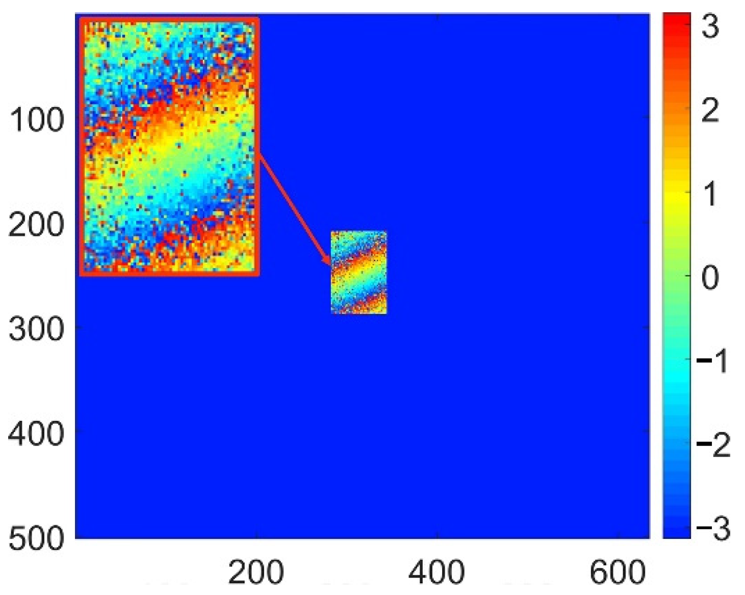
According to the calculated PSD matrix, the most central element is taken as the seed point, and $t$ percentage of the variance of the PSD matrix is used as the seed growth threshold ($t$ can be adjusted with different amount of noise; it is experimentally set to 50 in this paper). A region-growing algorithm [46] is performed to obtain the clear stripe area in the cross-power spectrum matrix, and the smallest bounding rectangle of the area is cropped for subsequent processing. The phase matrix is shown in Figure 4.

2.3. Cross-Power Spectrum Matrix Dimensional Reduction

After the screening in the previous section, a clear area of the cross-power spectrum matrix is obtained, which can be used to estimate the displacement well. Since the two-dimensional cross-power spectrum matrix is difficult to do the phase unwrapping, thus, dimensional reduction processing has to be performed.

According to the basic principles of phase correlation, the rank of the cross-power spectrum matrix is one under the ideal conditions [47], so SVD strategy can be used to make a rank-one estimation, and then the dimensionality of cross-power spectrum matrix is reduced from 2 to 1. SVD is performed on the screened cross-power spectrum matrix, its first singular value is taken, and the corresponding left and right singular vectors are used to represent the ideal cross-power matrix. Assuming the area matrix selected in the previous section is A, SVD decomposition on this matrix is performed according to Equation (5):

$$\mathrm{A}=\mathrm{U}\times \mathrm{diag}\left({\mathsf{\sigma }}_1,{\mathsf{\sigma }}_2,\cdots ,{\mathsf{\sigma }}_{\mathrm{k}},0,\cdots \right)\times \mathrm{V}$$

(5)

where $\mathrm{U}=\left[{\mathrm{u}}_1,\cdots ,{\mathrm{u}}_{\mathrm{k}}|{\mathrm{u}}_{\mathrm{k}+1},\cdots ,{\mathrm{u}}_{\mathrm{m}}\right]$, ${\mathsf{\sigma }}_1>{\mathsf{\sigma }}_2>\cdots$, $\mathrm{V}=\left[{\mathrm{v}}_1,\cdots ,{\mathrm{v}}_{\mathrm{k}}|{\mathrm{u}}_{\mathrm{k}+1},\cdots ,{\mathrm{v}}_{\mathrm{n}}\right]$.

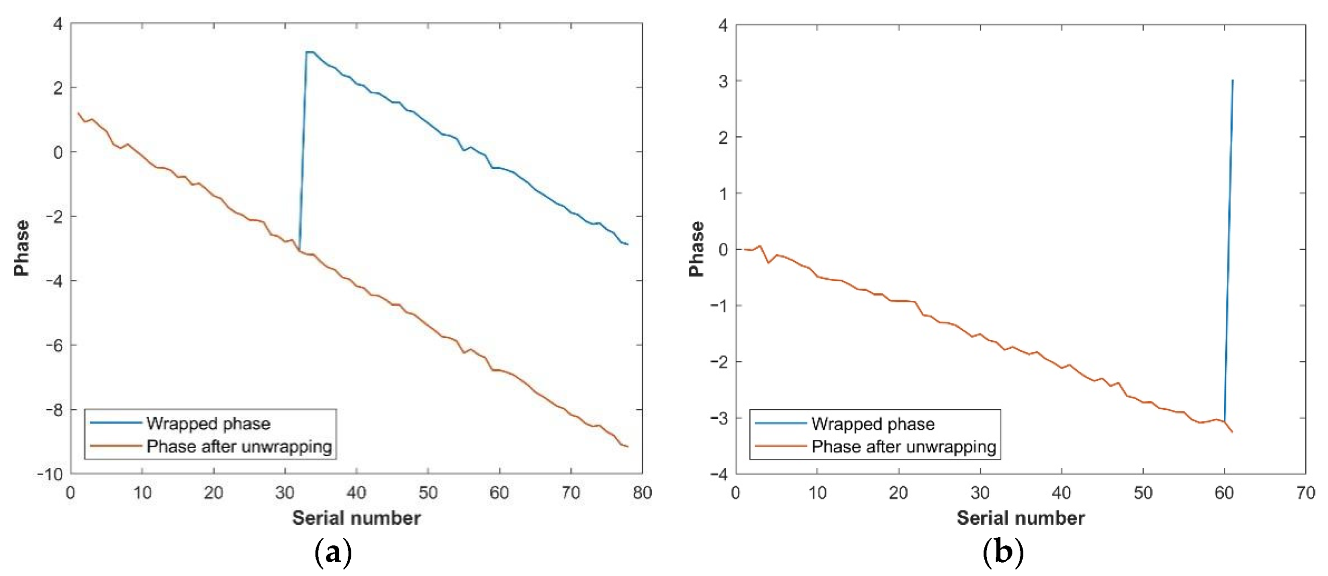
After SVD processing, the phase of corresponding left and right singular vectors ${\mathrm{u}}_1$ and ${\mathrm{v}}_1$ is calculated, and one-dimensional phase unwrapping is performed according to Equation (6). In this equation, ${\overline{\mathsf{\phi }}}_{\mathrm{i}}$ is the phase after unwrapping; ${\mathsf{\phi }}_{\mathrm{i}}$ is the currently processed phase; $\mathrm{mod}\left\{\mathrm{a},\mathrm{b}\right\}$ means taking the remainder of dividing $\mathrm{a}$ by $\mathrm{b}$; and ${\mathsf{\phi }}_0$ is the first phase in the sequence. The winding phases and unwrapping phases of ${\mathrm{u}}_1$ and ${\mathrm{v}}_1$ are shown in Figure 5, where Figure 5a is the winding phase and unwrapping phase of ${\mathrm{u}}_1$, and Figure 5b is the winding phase and unwrapping phase of ${\mathrm{v}}_1$:

$${\overline{\mathsf{\phi }}}_{\mathrm{i}}={\mathsf{\phi }}_0+{\displaystyle \sum }_{\mathrm{j}=0}^{\mathrm{i}-1}\mathrm{mod}\left\{\left({\mathsf{\phi }}_{\mathrm{j}+1}-{\mathsf{\phi }}_{\mathrm{j}}\right),2\mathsf{\pi }\right\}$$

(6)

2.4. Displacement Estimation Based on Straight-Line Fitting

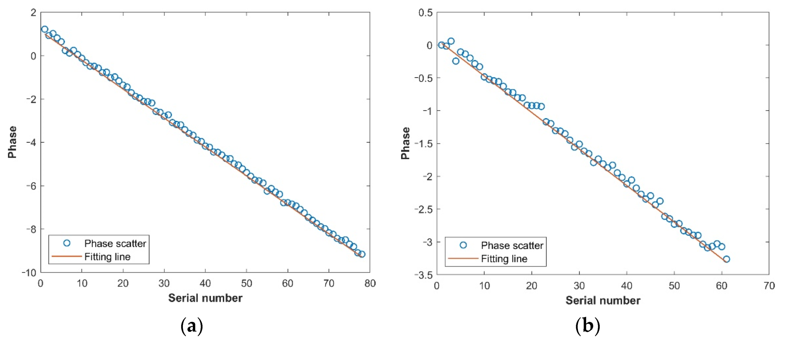
After the previous section, the phase scatter points used for displacement estimation have been obtained. Now, a straight-line fitting is required for the phase scatter points (as shown in Figure 6, where (a) is the unwrapping phase and straight-line fitting result of left singular ${\mathrm{u}}_1$, and (b) is the unwrapping phase and straight-line fitting result of right singular ${\mathrm{v}}_1$). According to the slope of the fitted line and the image size, the displacement is calculated by Equation (7).

$${\mathrm{X}}_0=-\frac{{\mathrm{k}}_{\mathrm{v}}\mathrm{W}}{2\mathsf{\pi }} {\mathrm{y}}_0=-\frac{{\mathrm{k}}_{\mathrm{u}}\mathrm{H}}{2\mathsf{\pi }}$$

(7)

where ${\mathrm{k}}_{\mathrm{u}}$ is the slope of the left singular vector phase fitting straight line; ${\mathrm{k}}_{\mathrm{v}}$ is the slope of the right singular vector fitting straight line; $\mathrm{W}$ is the image width; and $\mathrm{H}$ is the image height.

3. Experiment and Analysis

In order to verify the effectiveness of the proposed method, simulation and real data verification experiments are performed, and the results of the four typical existing phase correlation methods are also compared. The proposed method is implemented with Python. The experiments are performed on a desktop with i7 CPU and 16 G RAM. The camera used in the experiment is a Medvision MVSUA133GMT industrial camera. Some key parameters are shown in

Table 1. The parameters of the camera.

Parameter	Value
Sensor	1/2.7″ CMOS
Shutter type	Global shutter
Camera type	Black and white
Pixel size	4.0 × 4.0 μm
Effective pixels	1.3 million
Resolution at frame rate	1280 × 1024 at 245 FPS
Pixel bit depth	8 bit
Data interface	USB 3.0 Type B

. The lens used in the experiments has a variable focal length and variable aperture, which are convenient for setting different experimental conditions.

The simulation experiment uses images with different texture characteristics, artificially adding noise and simulated displacement; the real data verification experiment is carried out in a high-speed railway laboratory, and the track vibration during the experiment is captured by shooting the digital speckle pattern of the track plate.

In this paper, we compare the performance of the proposed method to four typical phase correlation methods: (1) the local up-sampling based method, (2) the SVD-based method, (3) the RANSAC-based method, and (4) the SVD + RANSAC-based method. For the local up-sampling-based methods, we first obtain the integer pixel displacement by classical phase correlation methods, then up-sample the images locally, finally obtaining subpixel displacement by using the classical phase correlation methods again. For the SVD-based methods, we first acquire the cross-power spectrum matrix, then perform SVD decomposition on it, and, finally, perform straight-line fitting on the left and right unwrapped singular vectors to obtain the displacement. For the RANSAC-based method, we first acquire the cross-power spectrum matrix, and then perform RANSAC-based straight-line fitting on a row and column of it to obtain the displacement. For the SVD + RANSAC-based method, we first acquire the cross-power spectrum matrix, then perform SVD on it, and, finally, perform RANSAC-based straight-line fitting on the left and right unwrapped singular vectors to obtain the displacement.

3.1. Simulation Experiment

3.1.1. Experimental Data

Six sets of panchromatic images with iron texture, cement texture, and soil texture, respectively, were captured, and the distance between the camera and the objects is around 10 m. The subpixel displacement was simulated, and noise was added by the following processing steps (as shown in Figure 7): (1) These images were cropped in the upper-left-corner area and the lower-right-corner area separately, and then two images with integer pixel displacement were obtained. The integer pixel displacement simulated is ${\mathrm{x}}_0^{\prime }=-11 \mathrm{pixels}$ and ${\mathrm{y}}_0^{\prime }=-21 \mathrm{pixels}$. (2) The two images were down-sampled at the same ratio, the down-sampling ratio was set to 0.5 in this paper, and then two images with subpixel displacement were obtained. The simulated displacement was ${\mathrm{x}}_0=-5.5 \mathrm{pixels}$ and ${\mathrm{y}}_0=-10.5 \mathrm{pixels}$, and the size of each image after processing was 502 × 634. (3) Gaussian noise was added to each image separately to complete the data production of the simulation experiment. The added Gaussian noise has a mean value of $0$ and a variance $\mathsf{\sigma }=255\times 5\%=12.75 \mathrm{pixels}$.

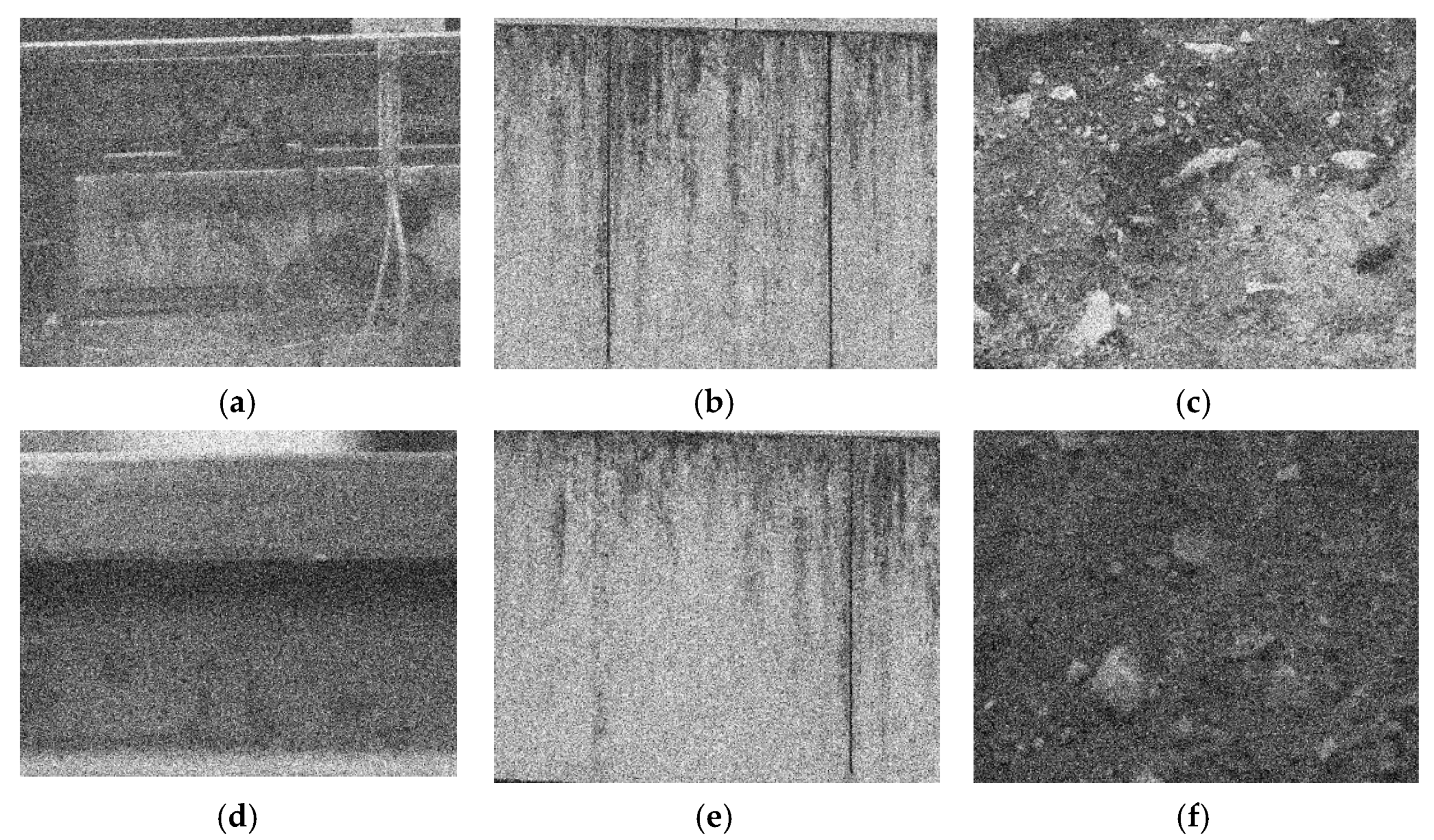
The simulated data obtained after these steps are shown in Figure 8, where (a) and (d) are iron textures, (b) and (e) are cement textures, and (c) and (f) are soil textures. It can be seen that the images used for the simulation experiment are seriously disturbed by noise, which makes it indeed challenging to estimate the displacement.

3.1.2. Results and Discussion

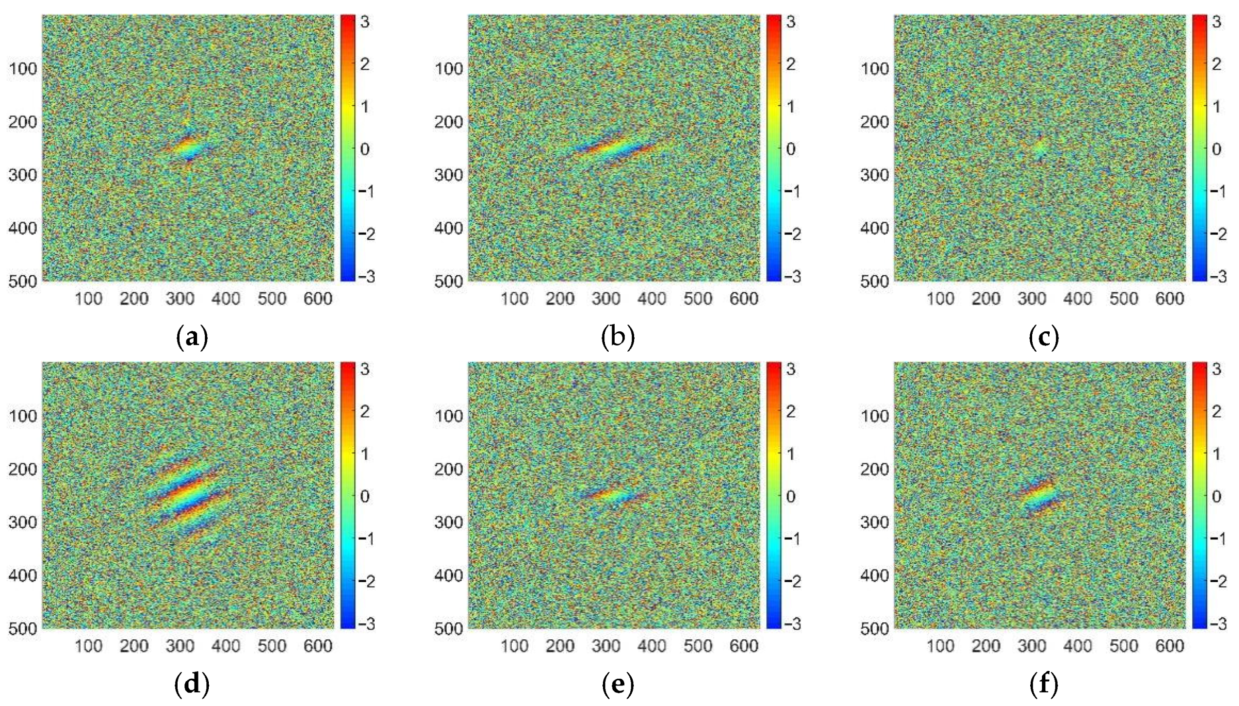
The six sets of images used in the simulation experiment were converted to the frequency domain using the two-dimensional discrete Fourier transform, then windowing was performed to prevent the spectrum from leaking, and, finally, two sets of images were converted to the frequency domain. Interferometric processing of the image can obtain the cross-power spectrum matrix. The phase of the cross-power spectrum matrix of the six sets of data are shown in Figure 9, where (a) and (d) are iron textures, (b) and (e) are cement textures, and (c) and (f) are soil textures. It can be seen from the spectrogram that the area with clear fringes in the spectrogram is very small due to severe noise interference, which makes displacement estimation a great challenge. At the same time, when the texture information of the image is not rich enough, such as the experimental data shown in Figure 8d, the frequency domain component brought by the texture information is even smaller than the frequency domain component caused by the noise, resulting in a smaller clear stripe area in the spectrogram. This further increases the difficulty of displacement estimation. Therefore, it is necessary to automatically filter out the regions with clear stripes in the spectrogram, which can improve the accuracy of the displacement estimation and the anti-interference ability of the displacement estimation against noise.

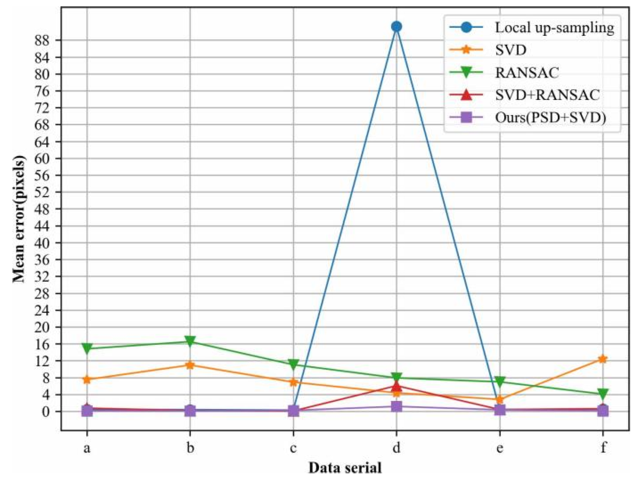
The five kinds of phase correlation methods mentioned above are used to estimate the displacement of the analog data. The absolute accuracy of the displacement results obtained by these five methods is shown in Figure 10 and

Table 2. Comparison of absolute accuracy of simulation experiments, where the unit is the pixel, and the bold font is the minimum error value among the five methods.

Methods	(a)	(b)	(c)	(d)	(e)	(f)
Local up-sampling	0.436	0.383	0.27	91.273	0.4	1.425
SVD	7.502	10.973	6.914	4.372	2.81	11.626
RANSAC	14.809	16.514	11.051	7.912	6.974	3.867
SVD + RANSAC	0.745	0.156	0.072	6.064	0.415	1.704
Ours (PSD + SVD)	0.135	0.087	0.202	1.153	0.341	0.479

. From the results, it can be seen that the proposed method is still able to estimate the displacement with high accuracy, even in the case of severe noise. At the same time, another interesting phenomenon can be seen from the experimental results: the absolute accuracy is about several to a dozen pixels, when using the SVD-based method or the RANSAC-based method alone. However, when combining SVD with RANSAC, the absolute accuracy of the displacement estimation is improved directly to the subpixel level. Of course, this is explainable: (1) When using the RANSAC algorithm for straight-line fitting, there is an important premise that the correct data accounts for the majority of all data; however, in the simulated data used in this paper, due to severe noise interference, the regions with clear stripes in the cross-power spectrum matrix also contain a certain percentage of noise. This leads to a small percentage of the correct data contained in the phase being used for straight-line fitting, which, in turn, makes the RANSAC-based method unable to obtain accurate displacement results. (2) When the SVD is used to process the cross-power spectrum matrix, there is also an important premise that the main component of the matrix is the correct information (stripes); however, due to the serious interference of noise, the main component of the cross-power spectrum matrix is not the correct information. This leads to the fact that SVD cannot fully recover the clear stripes in the whole region, which, in turn, makes the SVD-based method unable to obtain accurate displacement results. (3) When RANSAC is combined with SVD, the noise part is first removed from the clear-stripes region with the SVD strategy, so that the stripes are all correct information in the clear region; then RANSAC is used to fit the straight line, the correct straight line can be obtained, and the correct displacement result can be obtained; this is true even for the experimental data (c), where the noise is not particularly serious in comparison, as the data can acquire a better result than our method. However, when the noise is particularly serious, even if RANSAC is combined with SVD, the accuracy of the displacement results obtained is still inferior to our method.

From the result, it can be seen that among the three texture scenes, the accuracy of the proposed method performed best, especially for the steel-texture scene; the other four phase correlation methods can only obtain the displacement results with integer pixel accuracy, while the method in this paper can obtain subpixel precision displacement results. This is also interpretable. The essence of the phase correlation method is to use the texture changes of the photographed surface to perform correlation analysis. Therefore, the texture of the photographed surface needs to be rich enough to ensure sufficient correlation and obtain accurate displacement results. However, under the condition of a pure iron texture, the texture of the photographed surface is composed of the rust on the photographed surface and the surface itself, causing its texture to be far less rich than the cement texture or the soil texture. The proportion of areas with clear streaks is very small; that is, gross errors account for a large proportion of all the observed data. In this case, even if the RANSAC method against gross errors is used, accurate displacement results cannot be obtained. However, the method in this paper first removes the completely invisible areas of the cross-power spectrum matrix, and then performs subsequent displacement estimation to avoid the interference of the unclear areas of the cross-power spectrum matrix, so that accurate displacement results can be obtained.

In addition, it can also be seen that for the cement and soil scenes with rich-enough textures, the local up-sampling method and the SVD + RANSAC method can also obtain better displacement estimation accuracy, which indicates that in the case of sufficiently rich textures, the displacement estimation method using anti-gross error can also resist noise interference better. However, the accuracy of the proposed method is higher. This shows that it is effective, for a weak texture and a severe noise scene, to screen out the regions with clear fringes in the cross-power spectrum matrix first and then perform subsequent processing.

3.2. Real Data Verification

3.2.1. Experimental Data

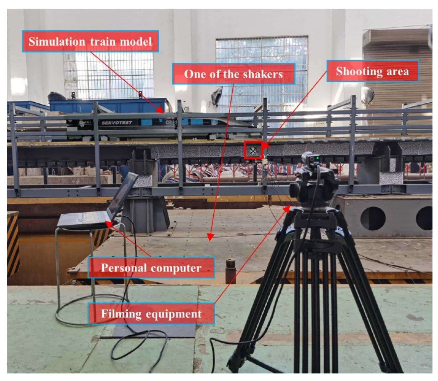
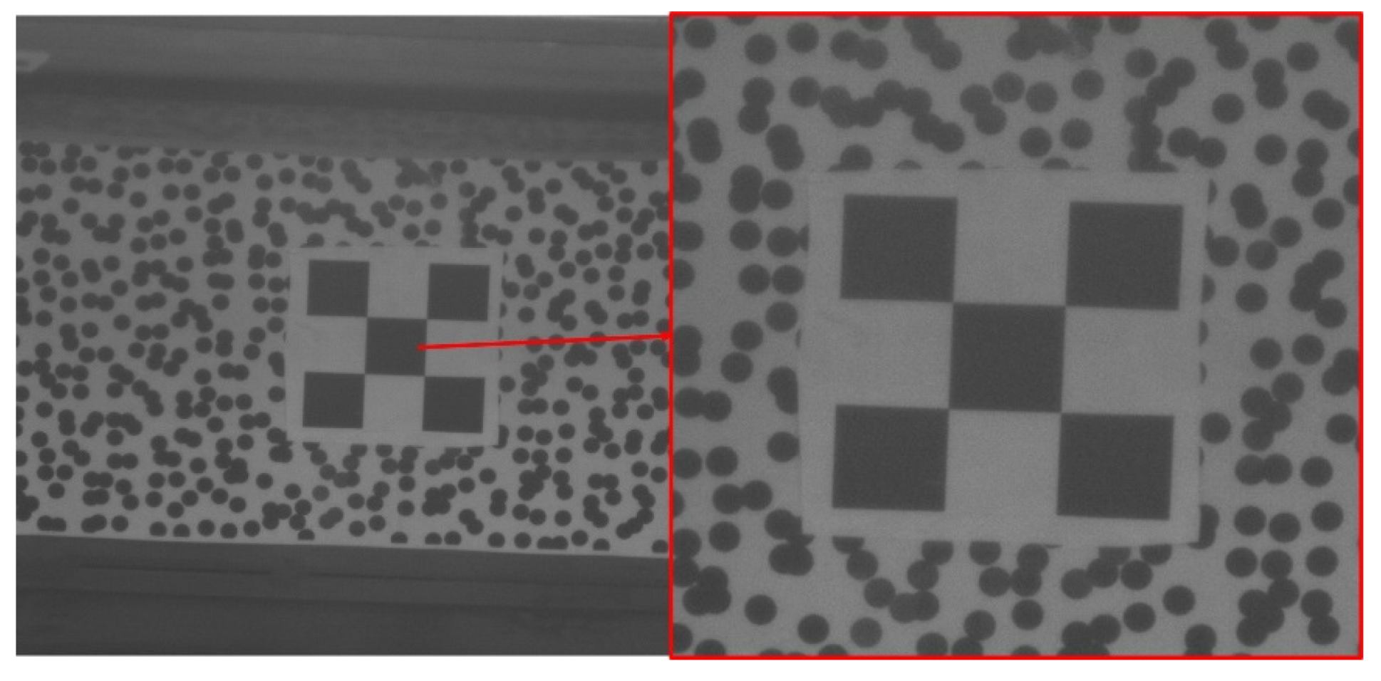
In order to further verify the accuracy of the proposed method, experiments were carried out in a high-speed railway multi-functional shaking-table test system. The experimental scene is shown in Figure 11, and one of the experimental images is shown in Figure 12; from the image, we can see that due to the high frequency of shooting, the image has serious noise. In this experiment, a displacement sequence was set to control the vibration of the shaking table to drive the bridge to vibrate. A high-frequency camera was used to obtain time-series images of the bridge vibrations. The above-mentioned five methods were used to calculate the displacement sequences, and then they were compared to the corresponding results with the vibration-table-control input sequence, to verify the accuracy of the proposed method.

The high-speed railway multi-function shaking-table test system consists of a 4 m × 4 m six-degree-of-freedom fixed table and three 4 m × 4 m six-degree-of-freedom mobile tables. The four shaking tables are all built on the same straight line and can be used independently or form a variety of spacing arrays. A single shaking table has the characteristics of three directions and six degrees of freedom, a large stroke, and a wide frequency band. The whole test system is mainly composed of the following parts: four sets of six-degree-of-freedom vibration tables (actuator, servo valve, differential pressure sensor, bearing, and steel platform); the adjustment system for the installation position of the movable table (support system, clamping system, winch system, and pipeline chain); a set of PULSAR double array digital control systems (servo controller, modulator, computer hardware/software, and uninterruptible power supply); hydraulic power source (hydraulic oil source, hydraulic oil source distributor, motors/pumps, accumulators, and oil–water heat exchangers), etc. The main technical parameters of the shaking table of the high-speed railway shaking-table test system are shown in

Table 3. Main technical parameters of shaking table of high-speed railway shaking-table test system.

Parameter	Value
Size (length × width)	4 m × 4 m
Number of degrees of freedom	3 directions and 6 degrees of freedom
Degree of freedom of two shakers’ linkage	12 degrees of freedom
The distance of two shakers	6–25 m (adjustable)
Maximum load	30 ton
Maximum displacement and maximum acceleration of X	250 mm, ±0.8 g (fully loaded)
Maximum displacement and maximum acceleration of Y	250 mm, ±0.8 g (fully loaded)
Maximum displacement and maximum acceleration of Z	160 mm, ±1.6 g (fully loaded)
Sine wave vibration speed	750 mm/s
Operating frequency range	0.1–50 HZ

.

During the experiment, four shaking tables were used to vibrate up and down synchronously, and the vibrations were transmitted to the simulated rail bridge to simulate a rail bridge under an earthquake state; a high-speed train was simulated by the proportional model of the high-speed locomotive. This paper uses a fixed shooting frequency of 200 HZ to shoot the track bridge, obtain the image data, and store it in a notebook connected to the camera. The camera distance was about 3 m from the lens to the monitoring surface. Before the vibrating table started to vibrate, the camera was turned on to shoot for a total of 30 s, and 5579 images were obtained (with a small frame drop phenomenon). The entire vibration process of the vibrating table was completely recorded in the images.

3.2.2. Results and Discussion

In total, 5579 images were processed by the five employed methods to obtain the displacement sequence of pixel units. Then, the real size of each pixel was calculated according to the real size $d_{real}$ of the target in the image and the pixel size ${\mathrm{d}}_{\mathrm{pixel}}$ of the target, according to Equation (8). In this paper, $d_{real}=20 \mathrm{mm}$ amd $d_{pixel}=142.014 \mathrm{pixels}$, so we obtain $d=0.141 \mathrm{mm}/\mathrm{pixel}$. 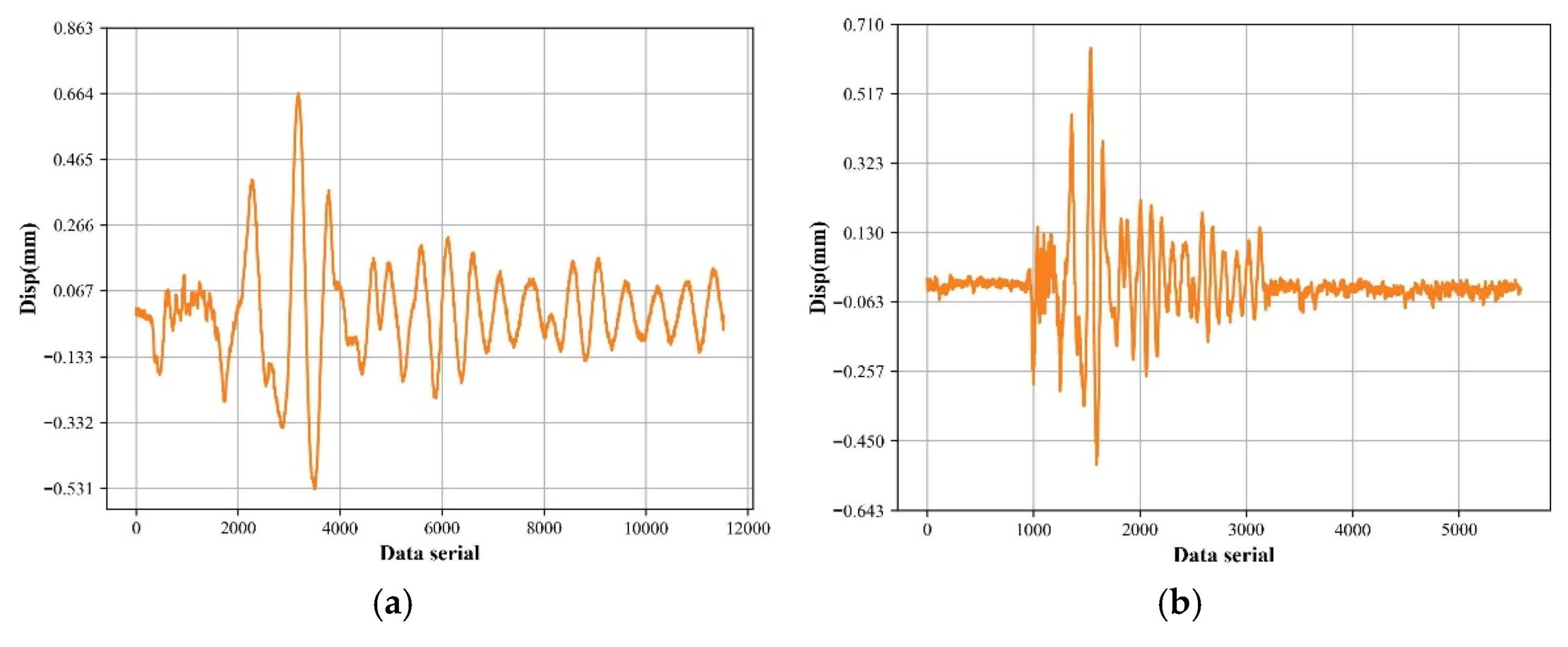According to the calculated scale parameters, the displacement sequence in pixel units is converted into millimeter units, and the displacement sequence is shown in Figure 13b.

$$d=\frac{d_{real}}{d_{pixel}}$$

(8)

In order to evaluate the accuracy of the displacement results obtained by the proposed method, the input displacement sequence used to control the vibration of the shaking table was derived and compared with the displacement sequence calculated by the proposed method. The derived original vibration input sequence of the shaking table is shown in Figure 13a.

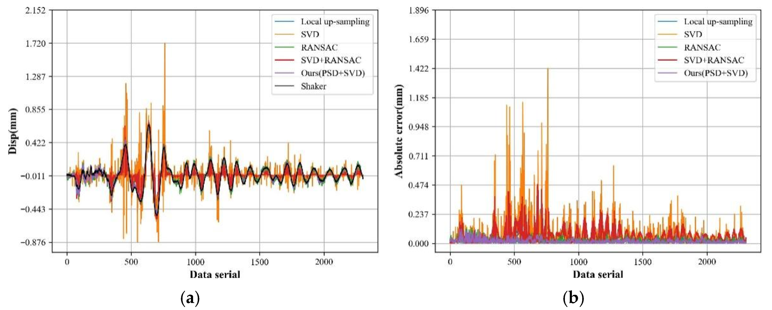
Since the input frequency is 1000 HZ, and the image shooting frequency is about 200 HZ, it is necessary to down-sample the displacement sequence of the shaking table to make the sampling frequency of the two sets consistent. At the same time, the collected image contains some non-vibrating parts on the shaking table, so it is necessary to locate the vibrating parts from the displacement sequence calculated by the proposed method, and then the corresponding accuracy can be evaluated. The processed displacement sequences calculated by these five phase correlation methods are shown in Figure 14a, the absolute error of those method is shown in Figure 14b, and the average absolute error is shown in

Table 4. Average absolute error of each phase correlation method, where the bold font is the minimum error value among the five methods.

Method	Average Absolute Error (mm)
Local up-sampling	0.041
SVD	0.085
RANSAC	0.024
SVD + RANSAC	0.064
Ours (PSD + SVD)	0.018

.

From the comparison chart of the displacement sequence (as shown in Figure 13a), the displacement sequence obtained by the improved phase correlation method proposed in this paper is consistent with the control sequence of the shaking table. From the comparison chart of the absolute error sequence (as shown in Figure 13b), it can be seen that the fluctuation is smaller, and the absolute error of our method is also smaller compared to the others. From the average absolute error (as shown in Table 4), the average absolute error of the displacement sequence calculated by our method is the smallest, and the experimental results show that the proposed PSD-based phase correlation method has the advantages of high precision and strong anti-noise performance.

In addition, from Figure 14 and Table 4, it can be found that: (1) The displacement results obtained by the SVD method have the worst accuracy, which indicates that in the case of severe noise, the use of SVD cannot restore the cross-power spectral matrix to a state of clean stripes, so the SVD method alone cannot obtain accurate displacement results; thus, it is necessary to combine the RANSAC method on this basis to obtain more accurate displacement results. (2) In this experiment, the photographed scene is sprayed with digital speckle, which enriches the texture of the scene. Therefore, even if there is a lot of noise under high-frequency shooting, the five methods in this experiment can obtain satisfactory accuracy. However, the method in this paper is still better, which further reveals that the proposed method is more resistant to noise. (3) In this experiment, the accuracy obtained by the SVD + RANSAC method is worse than that obtained by using the RANSAC method alone, which seems to be contrary to the conclusion obtained in the simulation experiment. This is due to the fact that the displacement that occurs is smaller compared with that of the simulation experiment. In the case of small displacement, the width of the stripes corresponding to the cross-power spectral matrix is larger (even larger than the image width or height), which leads to the clean stripes of the cross-power spectrum matrix restored by SVD being inaccurate (as shown in Figure 15, where (a) is the original cross-power spectrum matrix, and (b) is the cross-power spectrum matrix restored by using SVD); so, when SVD is used, the displacement obtained has less accuracy. This can also explain that the displacement obtained using the SVD method in this experiment has the worst accuracy.

4. Conclusions

The digital correlation method plays an import role in non-contact structure health monitoring. In this paper, a phase correlation method based on PSD phase screening is proposed for displacement estimation under severe noise interference. Through the use of PSD, regions with clear fringes can be effectively screened from the original interference phase, which provides a reliable data source for displacement estimation, using fringes in the subsequent steps. The simulated data experiments and high-speed rail laboratory experiments have validated the robustness of the proposed method.

By comparing with other typical four phase correlation methods, the experimental results show that the proposed method has high resistance to noise and can accurately estimate displacement in the case of serious noise interference, compared to the existing phase correlation methods.

Since the proposed method is a visual-based method, there are certain requirements for the monitoring scene: one is that the scene can be imaged; at the same time, it has to be ensured that the displacement size (pixels) will not exceed the detectable range of the phase correlation method. In general, the proposed method can be inserted as a module to an existing DIC tool, to monitor structures’ displacement that can be clearly imaged, and the imaging resolution can meet the accuracy requirements.

The proposed method can avoid noise affection. However, it is a method based on digital image, thus, if the images are not captured with an optimal light source, the promising results could not be obtained. In such situation, an auxiliary artificial light source is needed to ensure the image quality of the measured surface or targets.

The proposed method still needs to be improved in some aspects. When using PSD for phase screening, the excessive screening phenomenon may occur and generate a too-small screened area. That means the amount of data utilized for displacement estimation would be limited, resulting in unsatisfying estimation results. In addition, because the calculation process of PSD is time-consuming, the efficiency of the proposed method has to be improved in the future.