
Research on the Influence of Tractor Parameters on Shift Quality, Based on Uniform Design

Abstract
:1. Introduction
2. Powertrain Model
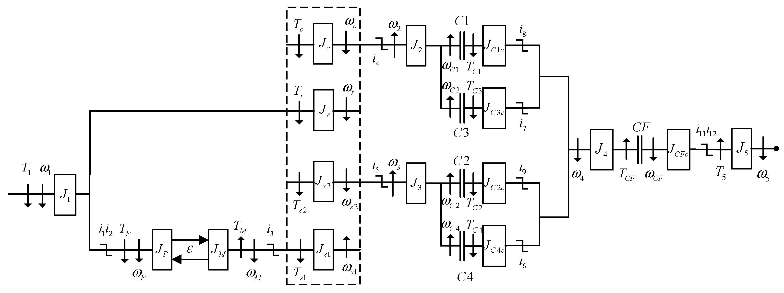
2.1. HMCVT Mechanical System
2.1.1. Rotational Dynamics of the HMCVT
2.1.2. Variable Displacement Pump-Fixed Displacement Motor System
2.1.3. Dynamic Clutch Friction Model
2.2. Longitudinal Tractor Dynamics
2.3. Hydraulic Component Actuation
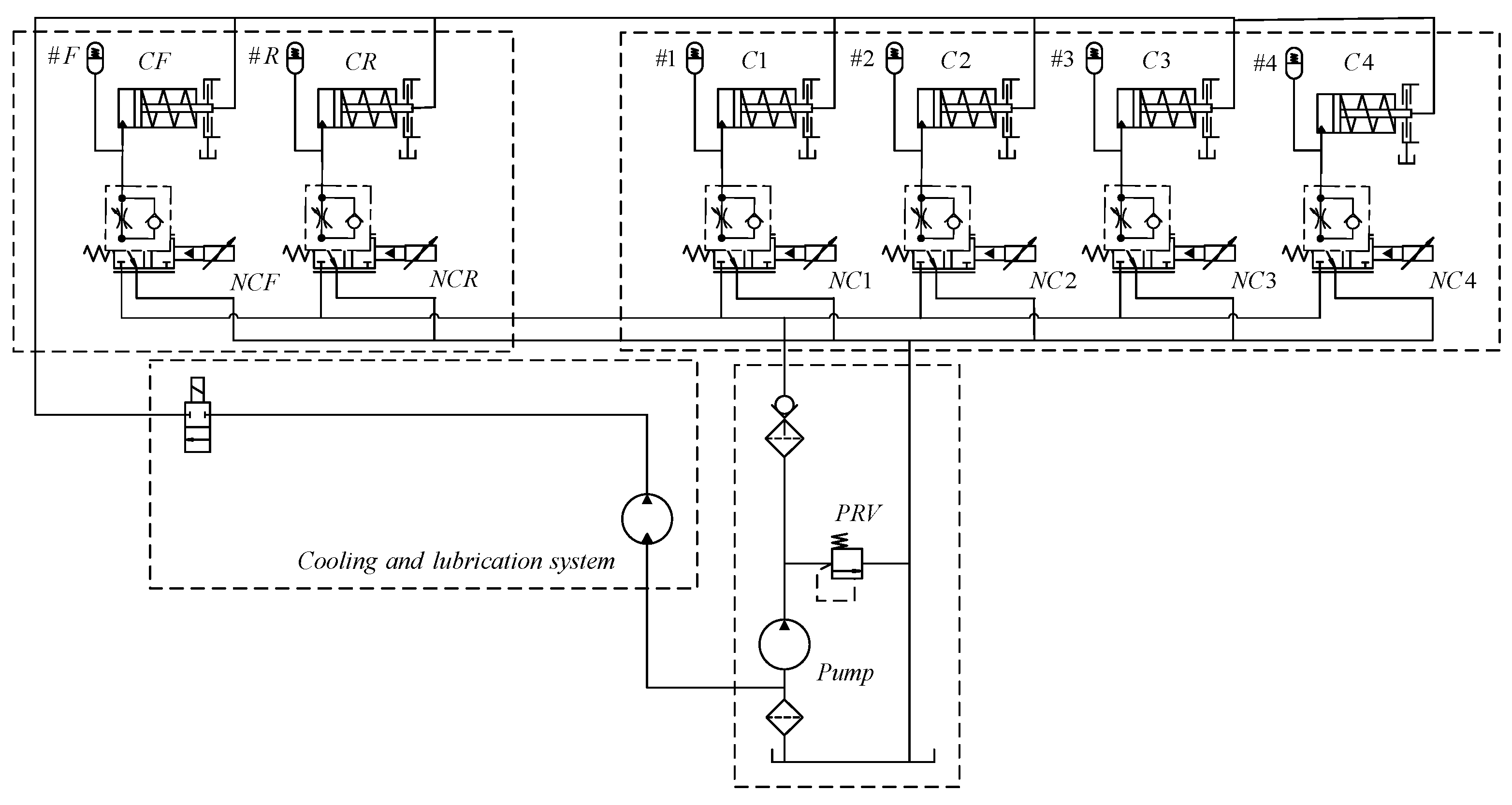
2.3.1. Pressure Regulation System
2.3.2. Clutch Actuation System
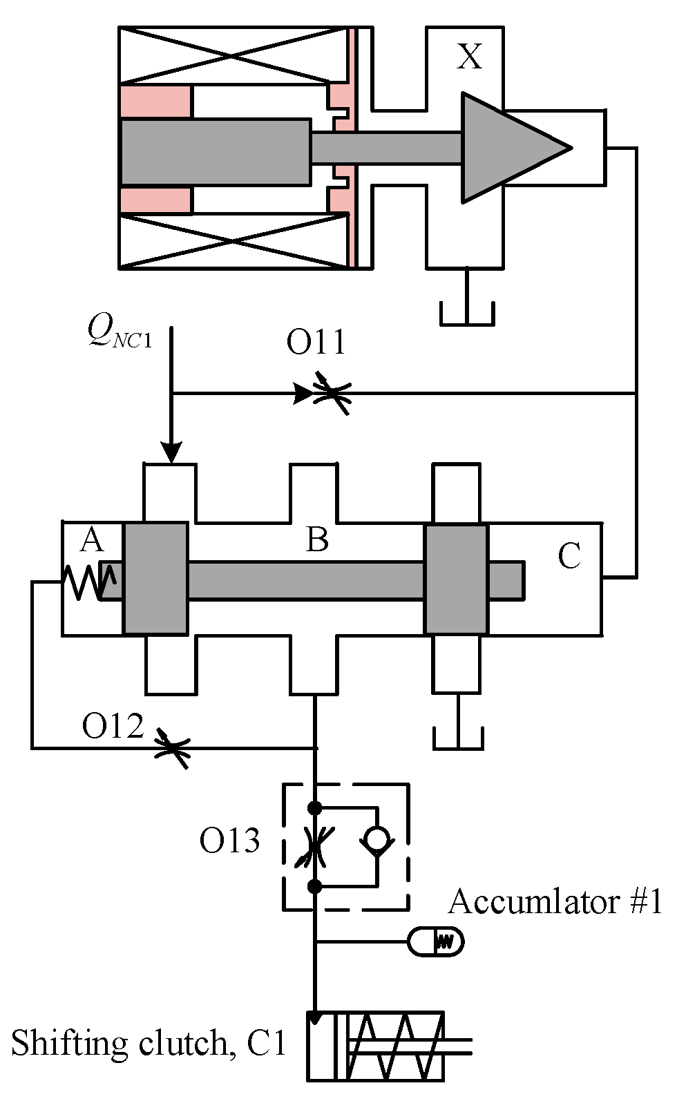
Pilot-Operated Proportional Pressure Reducing Valve (NC1)
- (1)
- Spool mechanical systems
- (a)
- Pilot valveThe pilot valve spool motion depended on the difference in pressure forces acting on the spool, the magnetic force, the inertia force, the viscous damping force, and the steady-state flow forces due to flow through the exhaust and inlet ports. The static friction force and the transient flow force were assumed to be negligible. Thus, the mechanical dynamics of the pilot valve were described by the following:where is the mass of the plunger, kg; is the viscous damping coefficient, N/(m/s); is the magnetic force acting on the spool, N; is the pressure in chamber X, Pa; is the land cross-sectional areas at chamber X, m2; is the spool displacement, m; and is the net steady flow force acting on the spool, N.
- (b)
- Main valveThe main valve spool motion depended on the difference in pressure forces acting on the spool, the net spring force, the inertia force, the viscous damping force, and the steady-state flow forces due to flow through the exhaust and inlet ports. The static friction force and the transient flow force were assumed to be negligible. Thus, the mechanical dynamics of the main valve were described by the following:where is the mass of the plunger, kg; is the viscous damping coefficient, Nm/rad/s; is the spring constant, N/mm; , are the pressures in chambers A and C, Pa; , are the land cross-sectional areas at chambers A and C, m2; is the spool displacement, m; and is the net steady flow force acting on the spool, N.
- (2)
- Electromagnetic circuitIn the range of the proportional electromagnetic force displacement characteristics, the output force equation of the proportional electromagnet was as follows:The given voltage current equation of the proportional electromagnet was as follows:where is the current-force gain coefficient of the proportional electromagnet, N/A; is the displacement-force gain coefficient of the proportional electromagnet, N/m. The value was very small: about 0. is the current in the coil, A; is armature displacement, m; is the coil resistance and the internal resistance of the amplifier, ; is the coil inductance, H; is the voltage amplification factor of the amplifier; and is the current feedback gain coefficient of the proportional electromagnet, V/A.
- (3)
- Fluid flow systemFor the simplified hydraulic system, the net volumetric flow rate to the NC1 actuator came from the flow rate exiting the safety valve, . By applying the continuity equation at the safety valve exit, the flow rate at the inlet of the NC1, and were described by the following:where , and are the flow rates to the proportional pressure reducing valves— and , respectively.
- (a)
- Pilot valveThe flow through chamber X of the NC1 was defined by applying the following continuity equation to the chamber:where is the total flow rate into chambers X and C, m3/s; is the flow coefficient; is the constant area of sharp-edged orifice 11, m2; is the density of the transmission fluid, kg/m3; is the transmission fluid bulk modulus, Pa; is the flow rate at the outlet of chamber X, m3/s; and is the volume of chamber X, m3.
- (b)
- Main valveThe flow through chamber, B, of the NC1 was defined by applying the following continuity equation to the chamber, while the clutch was either filling or exhausting:where is the volume of chamber B, m3; is the pressure in chamber B, Pa. and , are the metered flow rates at the output and the exhaust of , respectively.The flow into and out of chambers A and C was described by applying the continuity equation at those chambers. The resulting equations were given by the following:where and are the flow rates into or out of chambers A and C, m3/s; is the spool speed, m/s; and and are the volumes in chambers A and C, m3.
Clutch Piston C1
- (1)
- Clutch piston mechanical dynamicsThe C1 piston motion depended on the pressure force acting on the piston, they were as follows: the spring force, the inertia force, and the viscous damping force. The static friction force and the flow force were assumed to be negligible. Thus, the mechanical dynamics of the C1 piston were described by the following:where is the mass of the clutch piston, kg; is the viscous damping coefficient, N/(m/s); is the spring constant, N/mm; is the pressure acting area of the clutch piston, m2; is the pressure applied to the clutch piston, Pa; is the spring preload, and N; , is defined as piston displacement and measured from the unloaded static equilibrium, m.
- (2)
- Fluid flow systemThe net volumetric flow rate to or from the clutch piston cavity,, was determined by applying the continuity equation at the outlet of the clutch pressure regulation valve. Furthermore, was also equal to the flow rate across accumulator #1. The resulting expression was given by the following equations:
3. Simulation Analysis of the Shift Process
3.1. Evaluation Indexes of Shift Quality
3.1.1. Acceptable Jerk
3.1.2. Shift Time
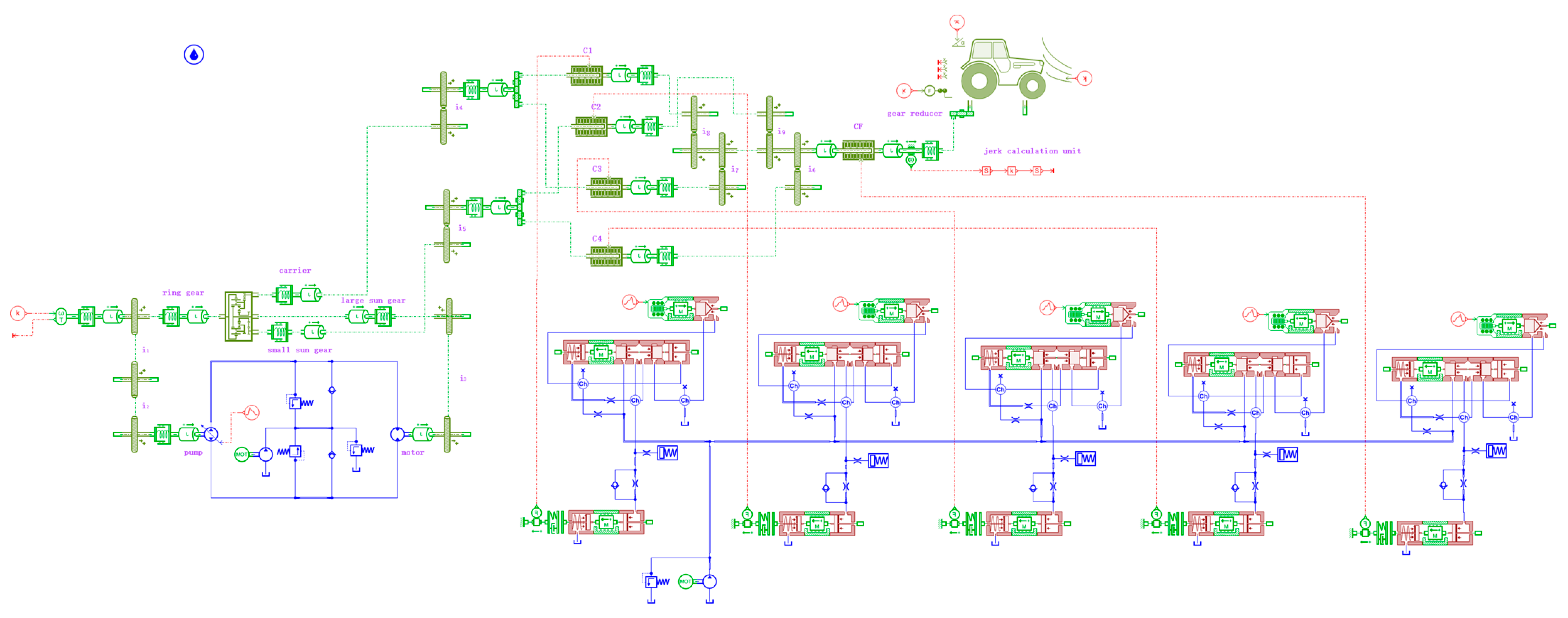
3.2. Simulation Model of Powertrain
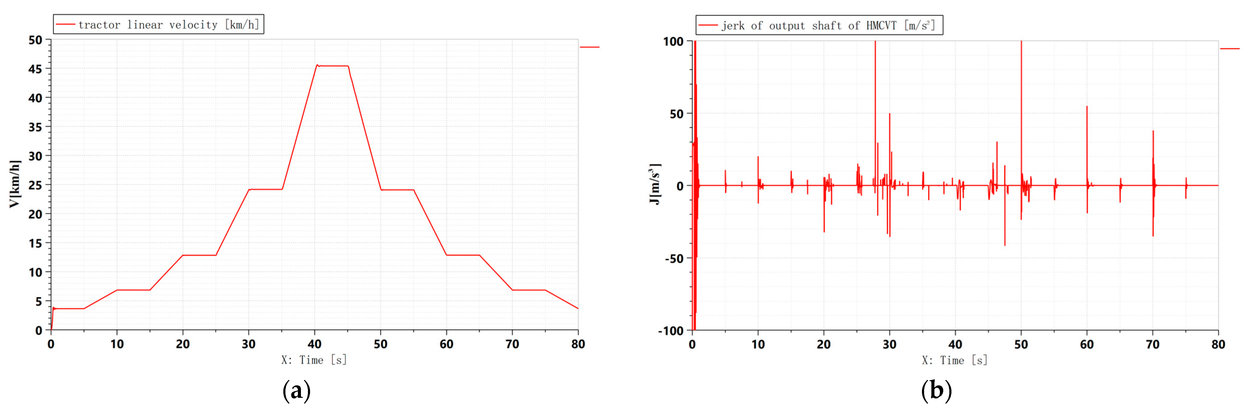
3.3. Continuous Shift Process of HMCVT
3.4. Analysis on the Influence of Tractor Parameters on the Shift Quality (Range 1 to Range 2)
3.4.1. The Shift Process under the Influence of a Single Parameter
- 1.
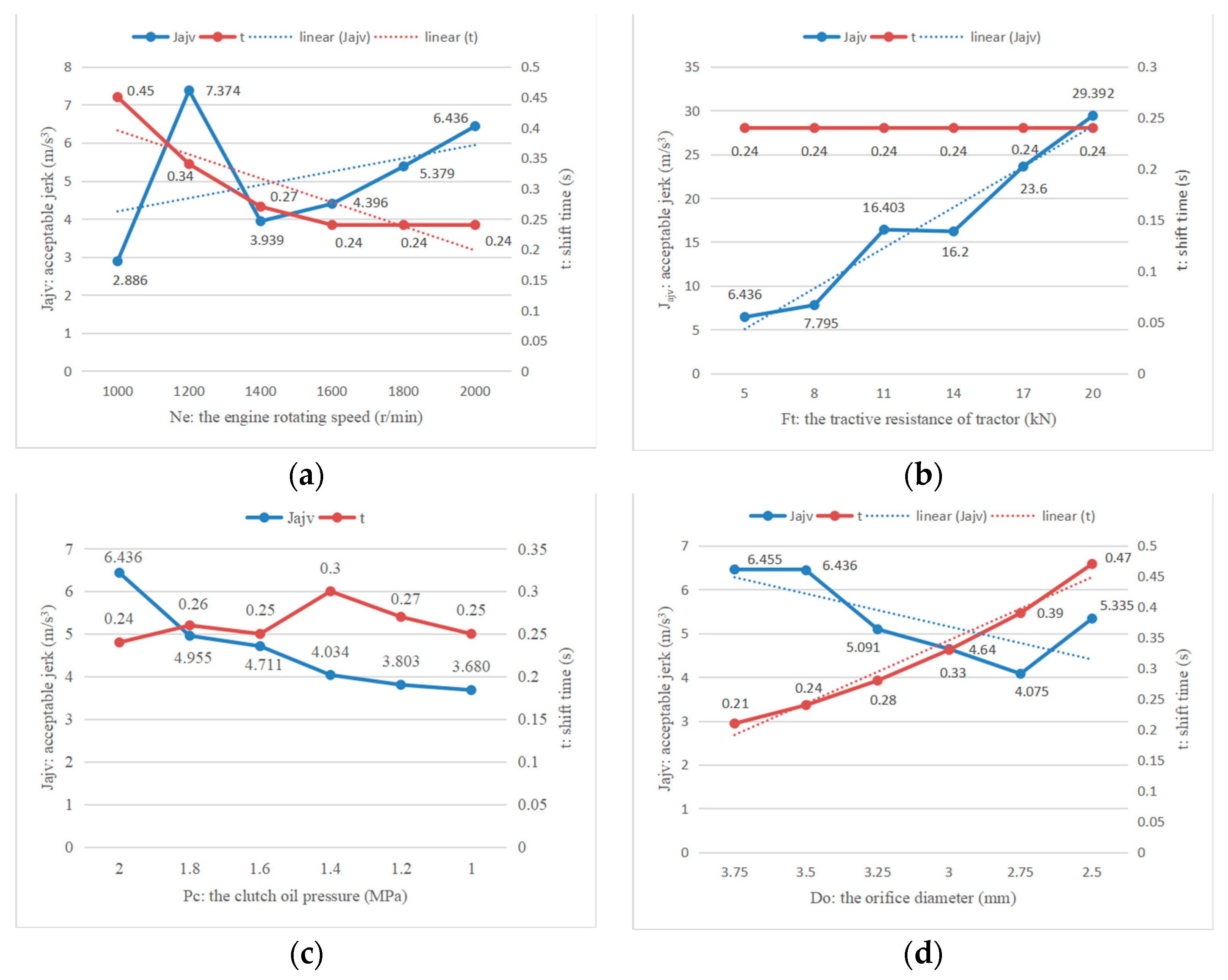
- Engine speedThe simulation condition can be expressed as follows: = 5 kN, = 2 MPa, = 3.5 mm. Six tests were conducted at engine speeds of 1000 r/min, 1200 r/min, 1400 r/min, 1600 r/min, 1800 r/min, and 2000 r/min. The test results are shown in Figure 7a. In general, the acceptable jerk value increased with the engine speed during the shift process. The shift time decreased with the increase in engine speed, and did not change after 0.24 s. Therefore, the engine speed had a significant effect on the acceptable jerk and shift time.
- 2.
- Tractive resistance of the tractorThe simulation condition can be expressed as follows: = 2000 r/min, = 2 MPa, = 3.5 mm. Six tests were conducted at the tractive resistances of the tractor of 5 kN, 8 kN, 11 kN, 14 kN, 17 kN, and 20 kN. The test results are shown in Figure 7b. The acceptable jerk value increased with the increase of the tractive resistances of the tractor during the shift process; the shift times were all 0.24 s. Therefore, the tractive resistance of the tractor had no effect on the shift time, but it had a significant effect on the acceptable jerk.
- 3.
- Clutch oil pressureThe simulation condition can be expressed as follows: = 2000 r/min, = 5 kN, = 3.5 mm. Six tests were conducted at the clutch oil pressure of 2 MPa, 1.8 MPa, 1.6 MPa, 1.4 MPa, 1.2 MPa, and 1 MPa. The test results are shown in Figure 7c. The acceptable jerk value decreased with the decrease of clutch oil pressure during the shift process. The shift time varied with the change of the clutch oil pressure during the shift process, but it did not reflect the regularity. Therefore, the clutch oil pressure had an irregular impact on the shift time and had a significant impact on the acceptable jerk.
- 4.
- Orifice diameterThe simulation condition can be expressed as follows: = 2000 r/min, = 5 kN, = 2 MPa. Six tests were conducted at the orifice diameters of 3.75 mm, 3.5 mm, 3.25 mm, 3 mm, 2.75 mm, and 2.5 mm. The test results are shown in Figure 7d. The acceptable jerk value decreased with the decrease of the orifice diameter, but if the orifice diameter was too small, it caused an increase in the acceptable jerk value. The shift time increased with the decrease of the orifice diameter. Therefore, the orifice diameter had a significant effect on the shift time and the acceptable jerk.
3.4.2. The Shift Process under the Influence of Combined Parameters
3.4.3. The Influence of Combined Parameters on Acceptable Jerk
3.4.4. The Influence of Combined Parameters on Shift Time
3.5. Discussion
4. Conclusions
Author Contributions
Funding
Institutional Review Board Statement
Informed Consent Statement
Data Availability Statement
Conflicts of Interest
Nomenclature
| Nomenclature | |
| lumped inertia, kg·m2 | |
| angular velocity, rad/s | |
| torque, Nm | |
| gear ratios | |
| displacement, cm3/r | |
| swash, | |
| high side pressure value of the pump-motor system, Pa | |
| low side pressure value of the pump-motor system, Pa | |
| volume of fluid on the high-pressure side, | |
| oil bulk modulus, Pa | |
| Stribeck constant (positive value), r/min | |
| maximum transmittable torque during sliding, Nm | |
| maximum transmittable torque during stiction, Nm | |
| relative velocity, rad/s | |
| tractor mass, kg | |
| radius of driving wheel, m | |
| speed of driving wheel, rad/s | |
| driving wheel torque, Nm | |
| road load torque, Nm | |
| wheel braking torque, Nm | |
| Q | volumetric flow rate, m3/s |
| P | Pressure, Pa |
| engine speed, rad/s | |
| pressure relief valve gain, m3/s/Pa | |
| line pressure, Pa | |
| cracking pressure, Pa | |
| mass of the plunger in pilot valve, kg | |
| viscous damping coefficient in pilot valve, N/(m/s) | |
| spool displacement in pilot valve, m | |
| magnetic force acting on the spool, N | |
| net steady flow force acting on the spool in pilot valve, N | |
| land cross-sectional areas, m2 | |
| mass of the plunger in main valve, kg | |
| viscous damping coefficient in main valve, N/(m/s) | |
| spool displacement in main valve, m; spool speed in main valve, m/s | |
| spring constant, N/mm | |
| net steady flow force acting on the spool in main valve, N | |
| current-force gain coefficient of the proportional electromagnet, N/A | |
| current in the coil, A | |
| displacement-force gain coefficient of the proportional electromagnet, N/m | |
| armature displacement, m | |
| proportional electromagnet voltage, V | |
| voltage amplification factor of the amplifier | |
| coil resistance and the internal resistance of the amplifier, | |
| current feedback gain coefficient of the proportional electromagnet, V/A | |
| coil inductance, H | |
| flow rate exiting the safety valve, m3/s | |
| total flow rate into chambers X and C of the NC1 | |
| flow coefficient | |
| constant area, m2 | |
| density of the transmission fluid, kg/m3 | |
| mass of the clutch piston, kg | |
| viscous damping coefficient, Nm/rad/s | |
| spring constant, N/mm | |
| pressure acting area of the clutch piston, m2 | |
| spring preload, N | |
| piston displacement, m; piston speed, m/s;piston acceleration, m/s2 | |
| , | jerk, peak jerk, root mean square jerk, |
| acceptable jerk, | |
| shift time, s | |
| engine speed, r/min | |
| tractive resistance of tractor, kN | |
| clutch oil pressure, MPa | |
| orifice diameter, mm | |
| Observed Response Value | |
| ,,, | regression coefficients |
| random error | |
| Subscripts | |
| 15 | shaft 1 shaft 5 |
| shifting clutches | |
| directional clutch | |
| large sun gear | |
| small sun gear | |
| ring gear | |
| carrier | |
| variable displacement pump | |
| fixed displacement motor | |
| PRV | pressure relief valve |
| NC1, NC2, NC3, NC4, NCF, NCR | pilot-operated proportional pressure reducing valve |
| NC1,X/A/B/C | chambers X/A/B/C of the NC1 |
| NC1,in | inlet of the NC1 |
| inlet or outlet of chamber X of the NC1 | |
| sharp-edged orifice11, 12, 13 | |
| control outlet of the NC1 | |
| exhaust of the NC1 |
References
- Macor, A.; Rossetti, A. Optimization of hydro-mechanical power split transmissions. Mech. Mach. Theory 2011, 46, 1901–1919. [Google Scholar] [CrossRef]
- Macor, A.; Rossetti, A. Fuel consumption reduction in urban buses by using power split transmissions. Energy Convers. Manag. 2013, 71, 159–171. [Google Scholar] [CrossRef]
- Rossetti, A.; Macor, A. Multi-objective optimization of hydro-mechanical power split transmissions. Mech. Mach. Theory 2013, 62, 112–128. [Google Scholar] [CrossRef]
- Zsolt, F.; György, K. Power flows and efficiency analysis of out- and input coupled IVT. Period. Polytech. Mech. Eng. 2009, 53, 61. [Google Scholar]
- Shamshirband, S.; Petkovic, D.; Amini, A.; Anuar, N.B.; Nikolić, V.; Ćojbašić, Ž.; Kiah, M.L.M.; Gani, A. Support vector regression methodology for wind turbine reaction torque prediction with power-split hydrostatic continuous variable transmission. Energy 2014, 67, 623–630. [Google Scholar] [CrossRef]
- Rotella, D.; Cammalleri, M. Power losses in power-split CVTs: A fast black-box approximate method. Mech. Mach. Theory 2018, 128, 528–543. [Google Scholar] [CrossRef]
- Tanelli, M.; Savaresi, S.M.; Manzoni, V.; Monizza, F.; Taroni, F.; Mangili, A. Estimating the maneuver quality of an automatic motion inverter for end-of-line tuning in agricultural tractors. IFAC Proc. Vol. 2008, 41, 10726–10731. [Google Scholar] [CrossRef] [Green Version]
- Park, Y.; Kim, S.; Kim, J. Analysis and verification of power transmission characteristics of the hydromechanical transmission for agricultural tractors. J. Mech. Sci. Technol. 2016, 30, 5063–5072. [Google Scholar] [CrossRef]
- Raikwar, S.; Tewari, V.K.; Mukhopadhyay, S.; Verma, C.R.; Rao, M.S. Simulation of components of a power shuttle transmission system for an agricultural tractor. Comput. Electron. Agric. 2015, 114, 114–124. [Google Scholar] [CrossRef]
- Hu, J.; Wei, C.; Yuan, S.; Jing, C. Characteristics on hydro-mechanical transmission in power shift process. Chin. J. Mech. Eng. 2009, 22, 50–56. [Google Scholar] [CrossRef]
- Linares, P.; Meńdez, V.; Catalań, H. Design parameters for continuously variable power-split transmissions using planetaries with 3 active shafts. J. Terramechanics 2010, 47, 323–335. [Google Scholar] [CrossRef] [Green Version]
- Kim, J.; Kang, J.; Kim, Y.; Min, B.; Kim, H. Design of power split transmission: Design of dual mode power split transmission. Int. J. Automot. Technol. 2010, 11, 565–571. [Google Scholar] [CrossRef]
- Cammalleri, M.; Rotella, D. Functional design of power-split CVTs: An uncoupled hierarchical optimized model. Mech. Mach. Theory 2017, 116, 294–309. [Google Scholar] [CrossRef]
- Wang, J.; Xia, C.; Fan, X.; Cai, J. Research on transmission characteristics of hydromechanical continuously variable transmission of tractor. Math. Probl. Eng. 2020, 2020, 6978329. [Google Scholar] [CrossRef]
- Kim, D.C.; Kim, K.U.; Park, Y.J.; Huh, J.Y. Analysis of shifting performance of power shuttle transmission. J. Terramechanics 2007, 44, 111–122. [Google Scholar] [CrossRef]
- Wang, G.; Zhang, X.; Zhu, S.; Zhang, H.; Tai, J. Dynamic simulation on shift process of tractor hydraulic power split continuously variable transmission during acceleration. Trans. Chin. Soc. Agric. Eng. 2016, 32, 30–39. [Google Scholar]
- Oh, J.Y.; Park, J.Y.; Cho, J.W.; Kim, J.G.; Kim, J.H.; Lee, G.H. Influence of a clutch control current profile to improve shift quality for a wheel loader automatic transmission. Int. J. Precis. Eng. Manuf. 2016, 18, 211–219. [Google Scholar] [CrossRef]
- Zhu, Z.; Gao, X.; Pan, D.; Zhu, Y.; Cao, L. Study on the Control Strategy of Shifting Time Involving Multigroup Clutches. Math. Probl. Eng. 2016, 2016, 9523251. [Google Scholar] [CrossRef]
- Zhu, Z.; Gao, X.; Cao, L.; Cai, Y.; Pan, D. Research on the shift strategy of HMCVT based on the physical parameters and shift time. Appl. Math. Model. 2016, 40, 6889–6907. [Google Scholar] [CrossRef]
- Armstrong-HéLouvry, B. Control of machines with friction. J. Tribol. 1991, 114, 637. [Google Scholar] [CrossRef] [Green Version]
- Watechagit, S. Modeling and Estimation for Stepped Automatic Transmission with Clutch-to-Clutch Shift Technology. Ph.D. Thesis, The Ohio State University, Columbus, OH, USA, 2004. [Google Scholar]
- Ni, X. Study on Features of Multisession and Double Row Confluence Hydromechanical Continuously Variable Transmission of Tractor. Master’s Thesis, Nanjing Agricultural University, Nanjing, China, 2013. [Google Scholar]
- Fang, K.T. Uniform Design and Uniform Design Table, 1st ed.; Science Press: Beijing, China, 1994; pp. 38–50. [Google Scholar]
- Zhuang, C.; He, C. Fundamentals of Applied Mathematical Statistics, 4th ed.; South China University of Technology Press: Guangzhou, China, 2013; pp. 387–398. [Google Scholar]


| Range | Directional Clutch | Shifting Clutch | Gearbox Gear Ratio (INPUT to Output Shaft) | Rear Axle Gear Ratio | |||||
|---|---|---|---|---|---|---|---|---|---|
| CF | CR | C1 | C2 | C3 | C4 | ||||
| Forward | First | + | + | 8.62∼4.59 | 20.72 | ||||
| Second | + | + | 4.59∼2.43 | ||||||
| Third | + | + | 2.43∼1.30 | ||||||
| Fourth | + | + | 1.30∼0.69 | ||||||
| Parameter | Value | Parameter | Value |
|---|---|---|---|
| (kg·m2) | 0.1283 | (kg·m2) | 0.2940 |
| (kg·m2) | 0.0940 | (kg·m2) | 0.2500 |
| (kg·m2) | 4.2333 | (kg·m2) | 0.0022 |
| (kg·m2) | 0.0040 | (kg·m2) | 0.0619 |
| (kg·m2) | 0.1893 | 1 | |
| −1.5 | , | −2 | |
| −0.825 | −0.580 | ||
| −2.046 | −2.920 | ||
| 1 | (Pa) | 1.7 × 10⁹ | |
| () | 6 × 10⁻⁴ | (cm3/r) | 54.8 |
| (cm3/r) | 54.8 | (kg·m2) | 0.0520 |
| (kg·m2) | 0.0060 | (kg) | 12,000 |
| (r/min) | 0.1 | (m) | 0.858 |
| Parameter | Value | Parameter | Value |
|---|---|---|---|
| (cm3/r) | 30 | (m3/s/Pa) | 8.33 × 10⁻⁷ |
| (Pa) | 2 × 10⁶ | (kg) | 0.01 |
| (N/(m/s)) | 10 | (kg) | 0.04 |
| (N/(m/s)) | 100 | (N/mm) | 10 |
| 0.7 | (kg/m3) | 850 | |
| (Pa) | 1.7 × 10⁹ | (kg) | 0.5 |
| (N/(m/s)) | 200 | (N/mm) | 438 |
| (N) | 500 | (m2) | 0.0217 |
| Test | Observed Response Value y | ||||
|---|---|---|---|---|---|
| 1 | 1000(1) | 8(2) | 1.4(3) | 3.75(6) | y1 |
| 2 | 1200(2) | 14(4) | 2(6) | 3.5(5) | y2 |
| 3 | 1400(3) | 20(6) | 1.2(2) | 3.25(4) | y3 |
| 4 | 1600(4) | 5(1) | 1.8(5) | 3(3) | y4 |
| 5 | 1800(5) | 11(3) | 1(1) | 2.75(2) | y5 |
| 6 | 2000(6) | 17(5) | 1.6(4) | 2.5(1) | y6 |
| Test | ||||||
|---|---|---|---|---|---|---|
| 1 | 1000(1) | 8(2) | 1.4(3) | 3.75(6) | 5.05 | 0.25 |
| 2 | 1200(2) | 14(4) | 2(6) | 3.5(5) | 11.44 | 0.34 |
| 3 | 1400(3) | 20(6) | 1.2(2) | 3.25(4) | 25.96 | 0.20 |
| 4 | 1600(4) | 5(1) | 1.8(5) | 3(3) | 3.82 | 0.28 |
| 5 | 1800(5) | 11(3) | 1(1) | 2.75(2) | 13.46 | 0.28 |
| 6 | 2000(6) | 17(5) | 1.6(4) | 2.5(1) | 19.23 | 0.41 |
| Source | Sum of Squares | df | Mean Square | F |
|---|---|---|---|---|
| Regression | 0.018 | 3 | 0.006 | 1.328 |
| Residual Error | 0.009 | 2 | 0.004 | |
| Total | 0.027 | 5 |
Publisher’s Note: MDPI stays neutral with regard to jurisdictional claims in published maps and institutional affiliations. |
© 2022 by the authors. Licensee MDPI, Basel, Switzerland. This article is an open access article distributed under the terms and conditions of the Creative Commons Attribution (CC BY) license (https://creativecommons.org/licenses/by/4.0/).
Share and Cite
Wang, J.; Xia, C.; Fan, X.; Cai, J. Research on the Influence of Tractor Parameters on Shift Quality, Based on Uniform Design. Appl. Sci. 2022, 12, 4895. https://doi.org/10.3390/app12104895
Wang J, Xia C, Fan X, Cai J. Research on the Influence of Tractor Parameters on Shift Quality, Based on Uniform Design. Applied Sciences. 2022; 12(10):4895. https://doi.org/10.3390/app12104895
Chicago/Turabian StyleWang, Junyan, Changgao Xia, Xin Fan, and Junyu Cai. 2022. "Research on the Influence of Tractor Parameters on Shift Quality, Based on Uniform Design" Applied Sciences 12, no. 10: 4895. https://doi.org/10.3390/app12104895
APA StyleWang, J., Xia, C., Fan, X., & Cai, J. (2022). Research on the Influence of Tractor Parameters on Shift Quality, Based on Uniform Design. Applied Sciences, 12(10), 4895. https://doi.org/10.3390/app12104895