The 3D Deburring Processing Trajectory Recognition Method and Its Application Base on Random Sample Consensus

Abstract

As of 2022, most automatic deburring trajectories are still generated using offline programming methods. The trajectories generated using these methods are often suboptimal, which limits the precision of the robotic arms used to perform automatic deburring and, in turn, results in workpiece dimensional errors. Therefore, despite advances in automated deburring trajectory generation, deburring is still mostly performed manually. However, manual deburring is a time-consuming, labor-intensive, and expensive process that results in small profit margins for organizational equipment manufacturers (OEMs). To address these problems and the obstacles to the implementation of automated deburring in the robotics industry, the present study developed an online automated deburring trajectory generation method that uses 2D contouring information obtained from linear contour scanning sensors, a CAD model, and curve fitting to detect burrs and generate appropriate trajectories. The method overcomes many of the limitations of common deburring methods, especially by enabling real-time trajectory tracking. When the method was tested using bicycle forks, work that originally took three to four people 8–12-h to complete was completed by one person in 30 min, and the production cost was reduced by 70%.

1. Introduction

According to an International Federation of Robotics (IFR) survey report, the demand for automated robotic arms is increasing at a compound annual growth rate of 19% and generating an annual output value of US$16.5 billion. The Industry, Science, and Technology International Strategy Center of Taiwan’s Industrial Technology Research Institute analyzed reports released by the International Federation of Robotics (IFR) [1] and International Monetary Fund (IMF) [2] and determined that a country’s industrial robot density indirectly affects its GDP per capita and manufacturing capacity. For example, on average, the doubling of industrial robot density in Germany and Japan would increase their respective GDPs per capita by 50%. By contrast, the doubling of industrial robot density in Taiwan would only increase its GDP per capita by 19%. This is because Taiwan primarily uses industrial robots for loading and unloading materials, and the effects of increases in robot density on GDP per capita are less profound. The main reason why only a small percentage of Taiwanese enterprises use robotic arms in high-end applications is that most enterprises in Taiwan’s robotics industry are small and medium-sized enterprises that cannot afford to incorporate high-end robotic arm applications or train technical personnel. To automate deburring, a series of robotic arm calibrations and compensations must be performed, and force control devices and offline programming software must be used to generate trajectories. These endeavors equate to software and hardware costs that total millions of dollars (NT$), and the resulting efficiencies also fail to meet industry demand. Therefore, deburring is mostly performed manually. Nevertheless, deburring has a high output value. For example, Taiwan’s metal factories manufacture approximately four million bicycle forks per year. Deburring after die casting is mainly performed manually, and bicycle forks produced after casting are subcontracted to and deburred by four organizational equipment manufacturers (OEMs), who are paid tens of millions of dollars (NT$). However, despite this high revenue, the profit margins enjoyed by these OEMs are small (of all the costs involved, labor accounts for approximately 80%). This, coupled with the fact that young people and foreign workers have been reluctant to venture into the manufacturing industry in recent years, has resulted in the OEMs encountering a labor shortage and evaluating the benefits of automatic deburring.

In metal and plastic molding and cutting operations, deburring is the least automated procedure and thus has the highest labor costs. Before deburring operations can be performed with current automatic deburring systems, the main body of the automated carrier, the tool center point, the tool axes, and the relationship between the carrier and the object to be processed must be calibrated. In addition, a series of offline programming software settings must be entered to generate projection trajectories. During processing, a control device is used to compensate for the dynamic errors in robotic arm movement (the robotic arm is in an open kinematic chain, and the end precision is thus easily affected during manufacturing and assembly; furthermore, the accuracy of joint torches and trajectories considerably affects the processing quality [3,4,5,6]) and deviations in workpiece dimensions.

As the manufacturing industry shifts from mass production with an economies-of-scale model to a customized business-to-consumer (B2C) model (i.e., producing small quantities of goods for large numbers of clients), how businesses can quickly generate processing trajectories for new products remains a question that must be answered before smart deburring can be realized. The main problems with implementing automated deburring in the context of the customized B2C model are as follows:

• Planning the trajectories of various workpieces offline is a costly, time-consuming, and labor-intensive process that cannot meet the manufacturing industry’s demand for rapid production of customized goods.
• Molding processes (such as plastic injection molding and metal casting molding) are affected by their environments. If large dimensional deviations occur during processing, workpieces may fail to maintain their fixed dimensions, and predetermined processing trajectories will not be applicable to all workpieces.

For highly customized manufacturing models, using offline programming to generate processing trajectories for a small number of workpieces and manually adjusting trajectories (which requires 3–8-h per workpiece) is a time-consuming process. The trajectories are also difficult to implement. Therefore, this study proposed an automatic deburring trajectory generation technique to achieve automatic adjustments and reduce operation time. During burr detection, curve fitting is performed using a computer-aided design (CAD) model of the target workpiece, and the curve information is obtained using linear contour scanning sensors, from which boundary contour curve equations are derived. The equations are used to detect burr distribution and generate processing point information, rapidly correcting processing trajectories to adapt to workpiece dimensional deviations and compensate for dynamic trajectory errors, thereby substantially enhancing the manufacturing flexibility of automatic deburring systems.

Many studies related to burr detection and online trajectory generation methods have been conducted. Most of these studies have applied pattern matching [7,8,9,10,11,12], force-sensing [13,14], stripe detection [15,16], edge recognition [17,18], and other [19,20,21] methods. When pattern matching is performed, the workpiece must be completely scanned to generate the processing trajectory because trajectory tracking for dynamic absolute error correction cannot be achieved during processing. In a force-sensing operation, force correction based on the processing situation can be conducted only after the processing trajectory is generated; therefore, the processing operation cannot be performed accurately when the workpiece size deviation is large (e.g., in the case of castings). Although the processing trajectory can be generated during processing in stripe detection and edge recognition, these methods can be used for burr detection only on edges and not curved surface areas (e.g., parting lines, gates, and risers) or irregular and discontinuous areas. Accordingly, existing trajectory generation methods cannot be effectively applied for burr removal after various processing procedures are performed. To address the aforementioned problems, an automated method was developed in this study for burr detection and deburring trajectory generation. This method enables online burr detection and deburring trajectory point extraction; that is, the dynamic accuracy of robotic arms and the workpiece size deviation can be compensated through burr tracking. Thus, the developed method solves the drawbacks of (and requires less processing time than do) current burr detection and online trajectory generation methods.

Although many burr detection and online trajectory generation method–related studies have been conducted, most have used methods involving pattern matching [3,4,5,6,7,8], force-sensing [9,10], stripe detection [11,12], edge recognition [13,14], and closed-loop compensation (with 3D measurement equipment) [15]. These methods generally can be applied only to detect burrs on edges and cannot be used to detect burrs on curved surface areas such as parting lines, gates, and risers or burrs that are irregular and discontinuous. To address this shortcoming, this study introduced a burr detection and automatic deburring trajectory generation method that enables burr trajectory tracking to solve the problems of low robotic arm dynamic accuracy and workpiece dimensional deviations.

This paper is organized as follows. Section 1 introduces the motivation and contribution of this study and the shortcomings of existing methods. Section 2 describes the proposed process for online 3D trajectory generation in deburring processing. This process involves extracting workpiece section contours and obtaining boundary equations by using laser contour scanning sensors to generate the deburring trajectory. Section 3 presents the results obtained in this study. Finally, Section 4 provides the conclusions of this study.

2. Online 3D Trajectory Generation for Deburring Processing

During metal processing, procedures such as casting, cutting, and forging create burrs on the surfaces of workpieces, which necessitates subsequent deburring. Because deburring performed by robotic arms is influenced by numerous variables (e.g., cast workpiece dimensional deviations, irregular burr distributions, and low robotic arm dynamic accuracy), deburring is still mainly performed manually. Although solutions to the aforementioned problems have been developed, automated deburring is expensive and time-consuming and requires a sufficient number of trained technicians to perform various preoperational processes, making large-scale use of automated deburring difficult. To address this problem, the method proposed herein uses automated carriers, deburring cutters, and linear contour scanning sensors to detect burrs and generate automatic deburring trajectories. In executing the method, a CAD model is used to analyze the cross-sectional contours of the workpiece and obtain the mathematical models for the contour curves. Subsequently, curve fitting is performed using linear scan information to obtain the boundary equations for detecting burrs online and generating deburring trajectories. The use of the burr trajectory tracking method can improve robotic arm dynamic accuracy and minimize workpiece dimensional deviations.

The proposed method comprises three stages. The first stage involves matching the mathematical model used for CAD-based cross-sectional contour feature extraction with that used for modeling boundary contour curves (S110, S120). The burr distribution is determined through linear contour scanning, and a mathematical model is established using cross-sectional contour data to obtain boundary equations and perform burr detection and trajectory generation. The second stage involves fitting the equations of boundary contour curves in linear contour scanning (S130, S140). Boundary contours are determined using linear contour scanning sensors to detect the actual position of the workpiece according to the manufacturing tolerance of the process, to compensate for the dynamic errors of robotic arms online, and to increase the control accuracy of robotic arms. The third stage involves detecting burrs and generating deburring trajectories (S150, S160). After the contour data obtained using linear contour scanning sensors are processed and curve fitting is completed, the cross-sectional boundary equations and the curves of the workpiece are obtained. These equations can be used to divide the space into two parts to detect the burr distribution and extract deburring trajectories. The procedures in the proposed method are described in Figure 1.

2.1. Matching the Mathematical Model

To detect burr distribution through linear contour scanning, mathematical models for curves must be established using cross-sectional contour information to obtain boundary equations. When the processing methods adopted for a target workpiece are known, a CAD model can be used to determine the regions where burrs must be removed. Cross-sectional images of the deburring regions must be obtained to derive the boundary contour curve model. The procedure is described as follows:

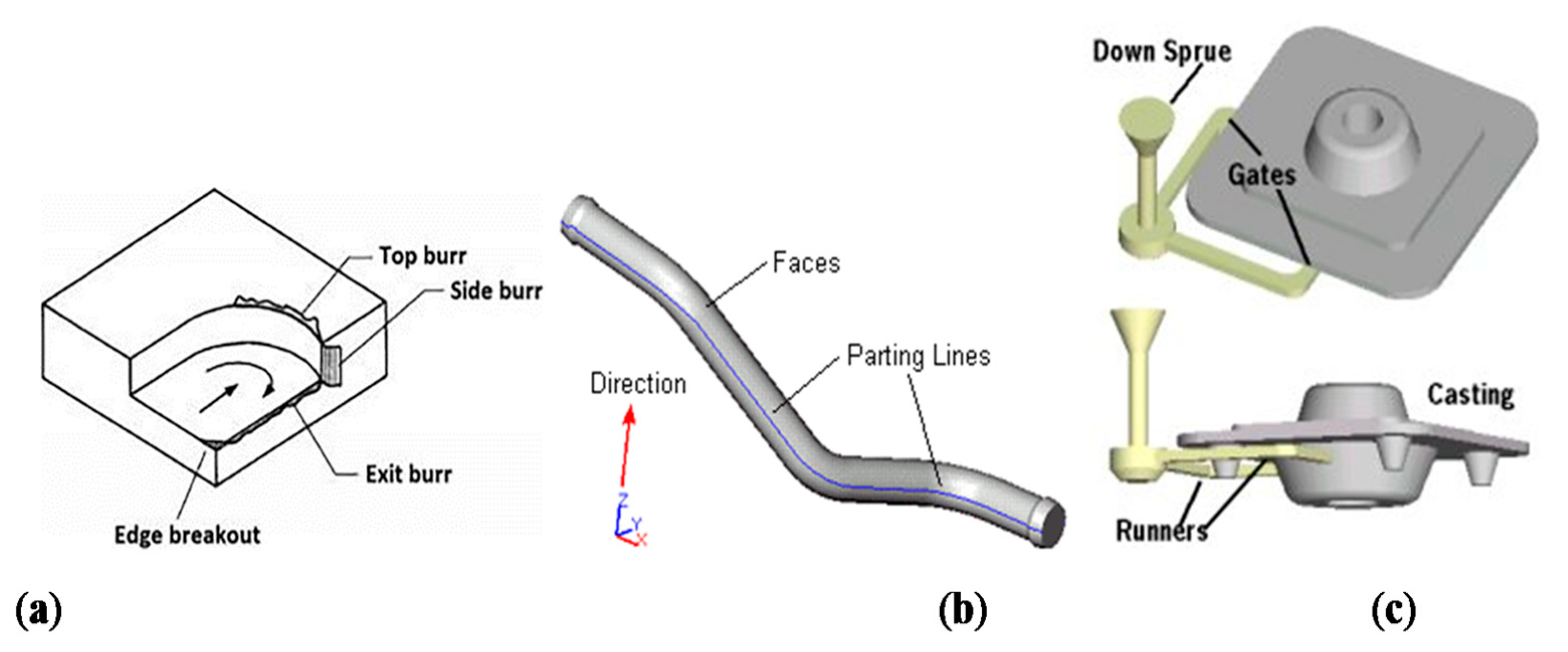
• The CAD model and target workpiece processing are analyzed to determine the deburring region. In workpieces that have undergone cutting, the deburring regions tend to be the processed edges. In those that have undergone casting, the deburring regions tend to include the gates, risers, and parting lines (Figure 2).
• The cross-sectional images of the deburring regions of the target workpieces along the cutting direction (e.g., the direction of the processed edge or parting lines) are obtained. To remove burrs on gates or risers, bow-shaped loops are used to plan surface-seeking trajectories. The contours are divided into n segments according to the cross-sectional contour curve characteristics, and the mathematical models for the different curves are determined accordingly. Because the characteristics of distinct cross-sectional boundary contour curves vary, their mathematical models vary. These models may include polynomial boundary curve equations, circular boundary curve equations, elliptic boundary curve equations, parabolic boundary curve equations, and square–ellipse boundary curve equations.
• The curve fitting errors are calculated and analyzed to determine whether they meet specific values (e.g., a coefficient of determination > 0.99).
  • For polynomial boundary curve equations, error analyses and model assessments can be performed using the coefficient of determination. Assuming that a dataset includes n observed values (i.e., $y_1,\cdots ,y_n$) and that the corresponding model-predicted values are $f_1,\cdots ,f_n$, respectively, the residual is defined as $e_i=y_i-f_i$, and the mean observed value is defined as $\overline{y}=\frac{1}{n}{\displaystyle \sum }_{i=1}^n{y}_i$.
  • The sum of squares of the observed and mean values are calculated using $S{S}_{tot}={\displaystyle \sum }_{i=1}^n{\left(y_i-\overline{y}\right)}^2$.
  • The residual sum of squares of the predicted and observed values obtained using the curve fitting model is calculated using $S{S}_{res}={\displaystyle \sum }_{i=1}^n{\left(y_i-f_i\right)}^2={\displaystyle \sum }_{i=1}^n{e}_i{}^2$.
  • For polynomial boundary curve equations, the coefficient of determination is $R^2=1-\frac{S{S}_{res}}{S{S}_{tot}}$.
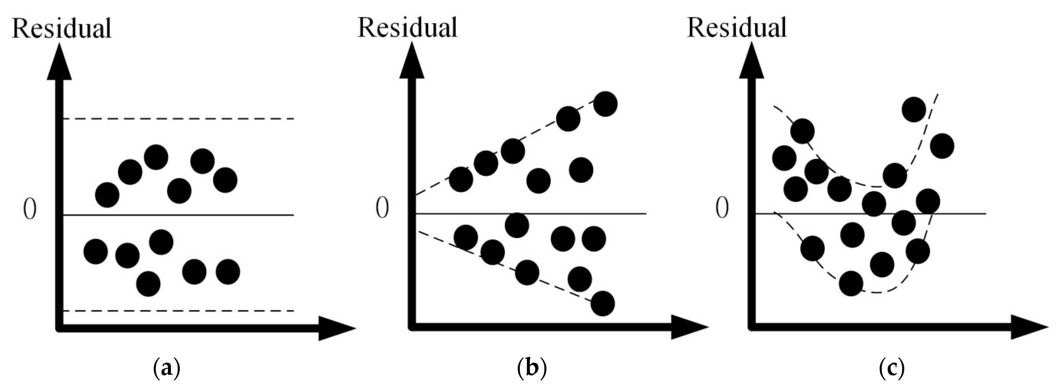
• Curve fitting residual plot analyses are performed to verify the accuracy of the residual distribution (Figure 3) according to the following criteria: (1) the residual value must be close to 0; (2) the residual points must be randomly and uniformly distributed between −1 and 1; (3) the residual point distribution must have no consistent pattern; and (4) the residuals must not contain any predictable information.
• The error analysis constraints, residual plot criteria, and minimum order equations comprise the curve-fitting model of the boundary equations.

2.2. Fit the Equations of Boundary Contour Curves (S130, S140) in Linear Contour Scanning

In metal and plastic processing, many processes (e.g., casting, forging, and injection molding) can be used to mold workpieces quickly. However, they also produce high engineering tolerances, resulting in large discrepancies between the actual workpiece dimensions and standard dimensions. When this happens, using the original contour curves obtained from the CAD model as the contours of the actual workpieces is impossible, and linear contour scanning sensors must be used to determine the boundary contours. This method can use the engineering tolerances obtained during processing to identify the actual workpiece contours, compensate for robotic arm dynamic errors online, and improve the precision of robotic arm control. The calculation procedure is as follows:

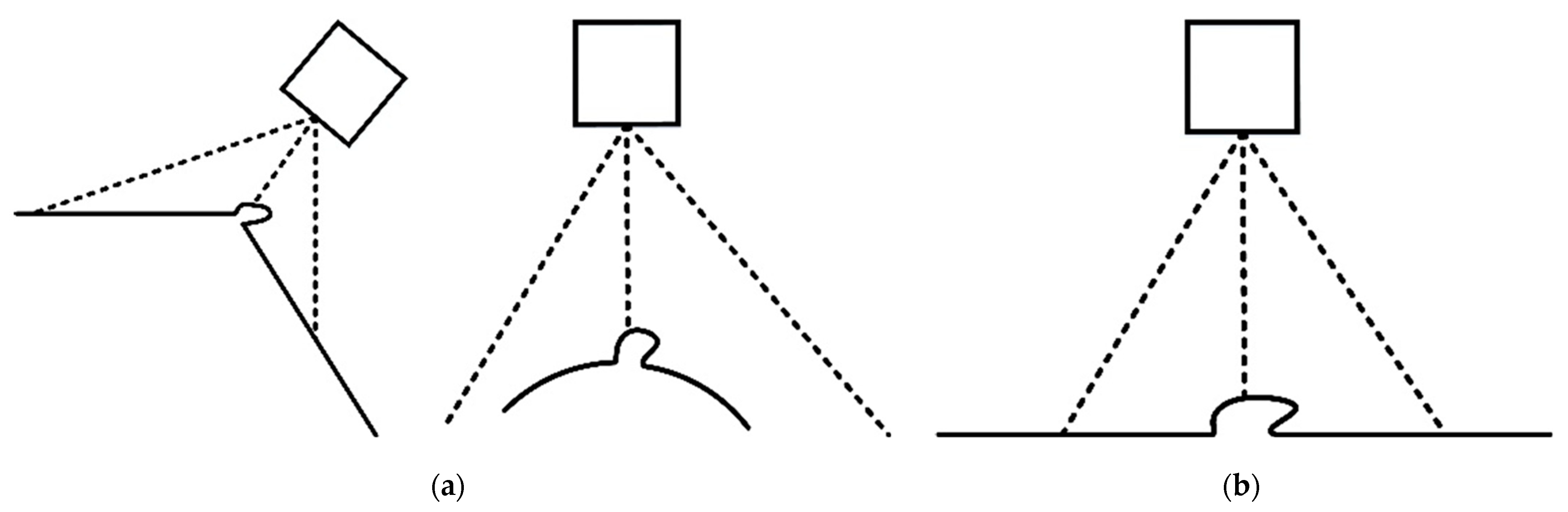
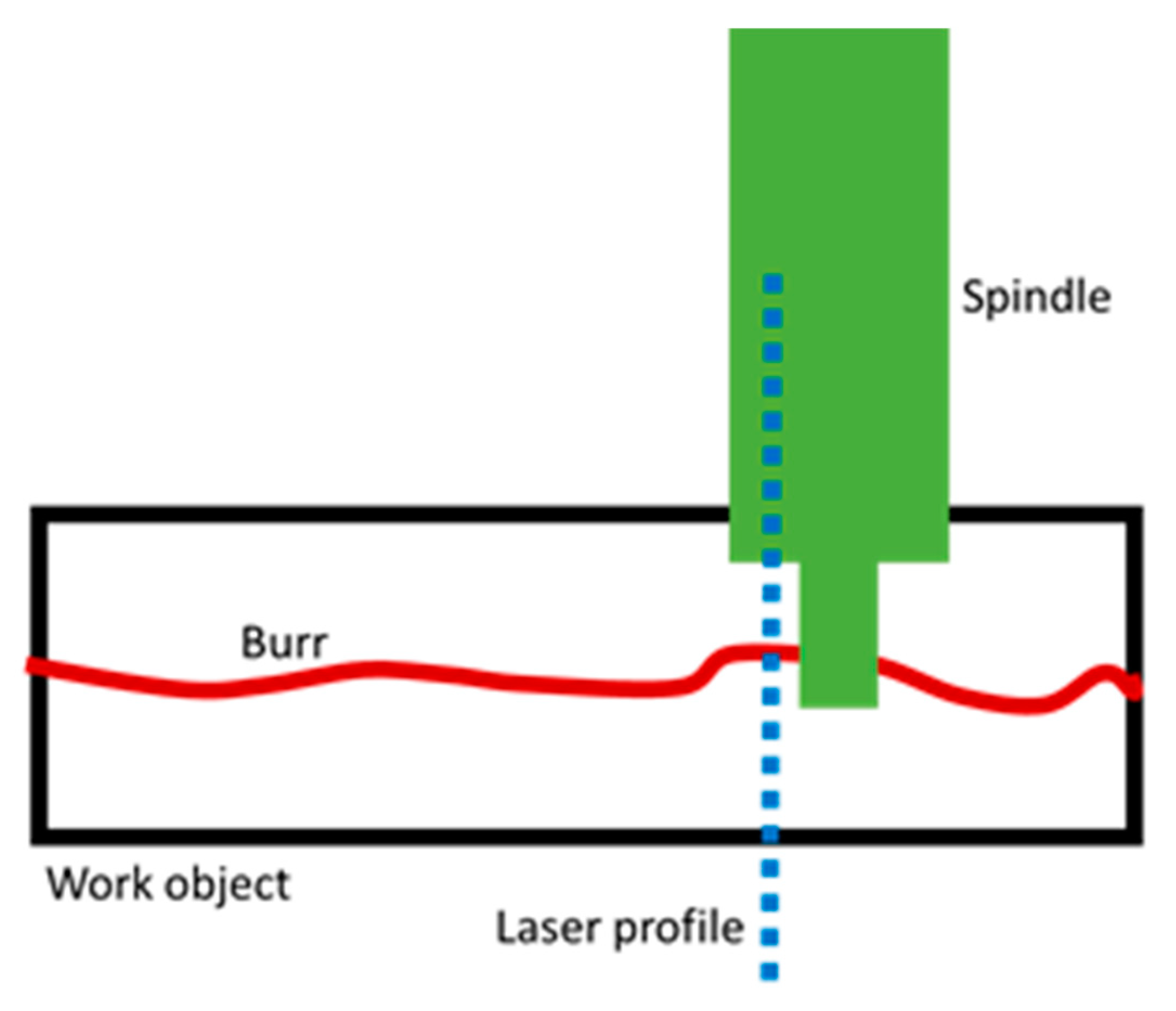
• After the mathematical models for the boundary contour curves of the target workpieces are determined, the workpiece contour cross-sectional information is obtained using linear contour scanning sensors. When the sensors move and scan the workpiece contours, they obtain as much information regarding the contours near burrs as possible by setting the burrs as the center of the scans (Figure 4).
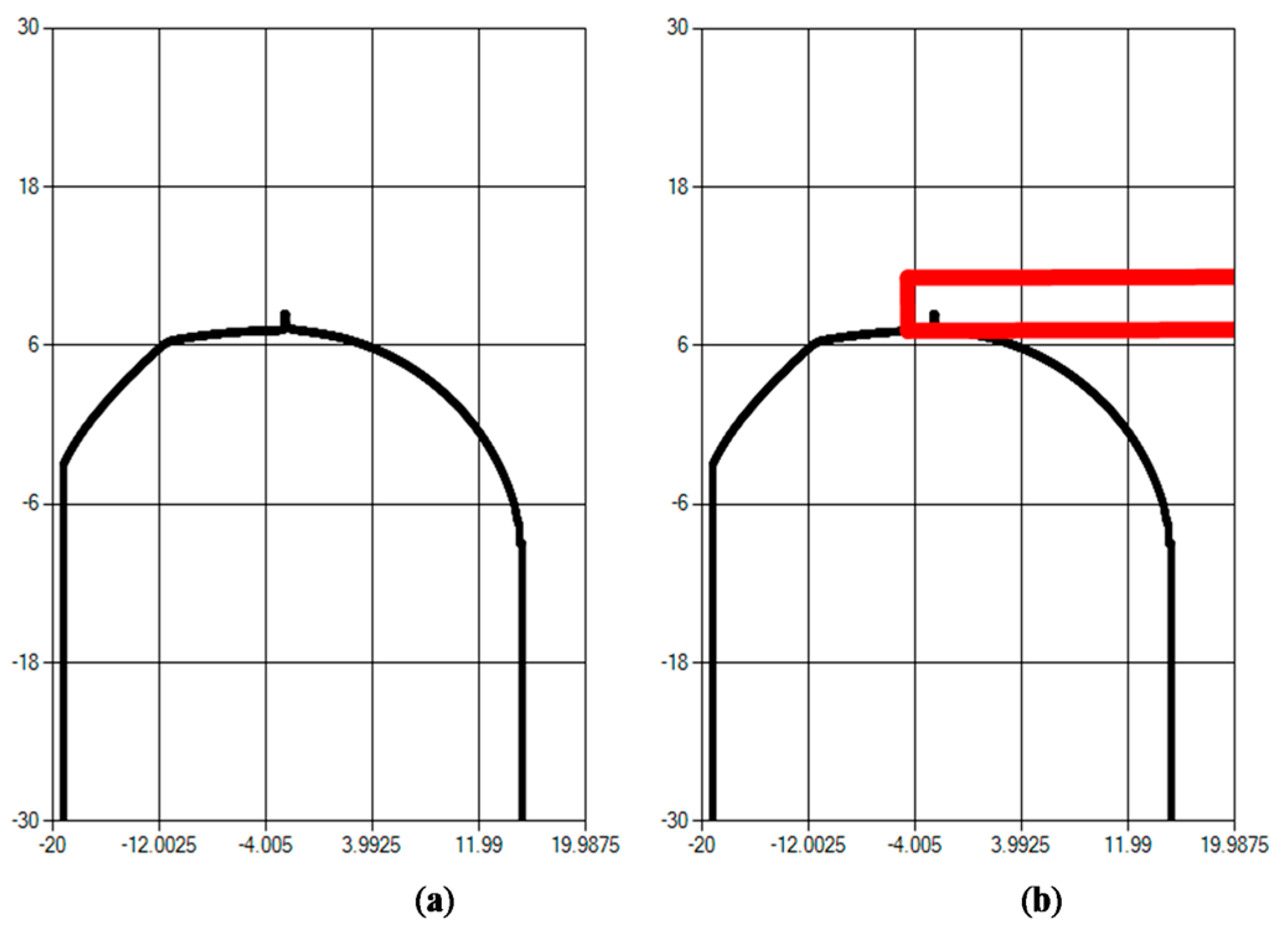
• The contour information obtained using the linear contour scanning sensors is processed, and the random sample consensus (RANSAC) method [22] is used to perform the fitting. This prevents burr information from influencing the curve fitting results.
  • Letting $i=0$, $t=0$, $m_{\mathrm{best}}=\mathrm{null}$, $f_{\mathrm{best}}=\mathrm{null}$, and $t_{\max }=\mathrm{null}$, the mathematical models for the boundary curves are selected (similar to Step 3).
  • A total of n samples are randomly selected, and the models are fit to obtain the curve equation $f_i$.
  • Letting $m_i=0$ and $n_i=0$, the data points are substituted into the curve equations to calculate the errors (${\mathsf{\delta }}_k$), where $m_i$ and $n_i$ are the number of interior points and exterior points, respectively.
  • ${\mathsf{\delta }}_k$ is compared with the allowable error ($\epsilon$): if ${\mathsf{\delta }}_k<\epsilon$, $m_i=m_i+1$; otherwise, $n_i=n_i+1$.
  • If $m_{\mathrm{best}}<m_i$, then $m_{\mathrm{best}}=m_i$ and $f_{\mathrm{best}}=f_i$.
  • When $t=t+1$, if $t_{\max }\ne \mathrm{null}$ and $t>t_{\max }$, the RANSAC procedure is performed with $t_{\max }$ as the number of iterations. If not, the number of iterations is updated to $t_{\max }=\frac{\log \left(1-P\right)}{\log \left(1-r^n\right)}$, where P is the expected probability of RANSAC obtaining the correct model, and r $\mathrm{is} \mathrm{the} \mathrm{ratio} \frac{m_i}{m_i+n_i}$, which is based on the numbers of interior and exterior points.
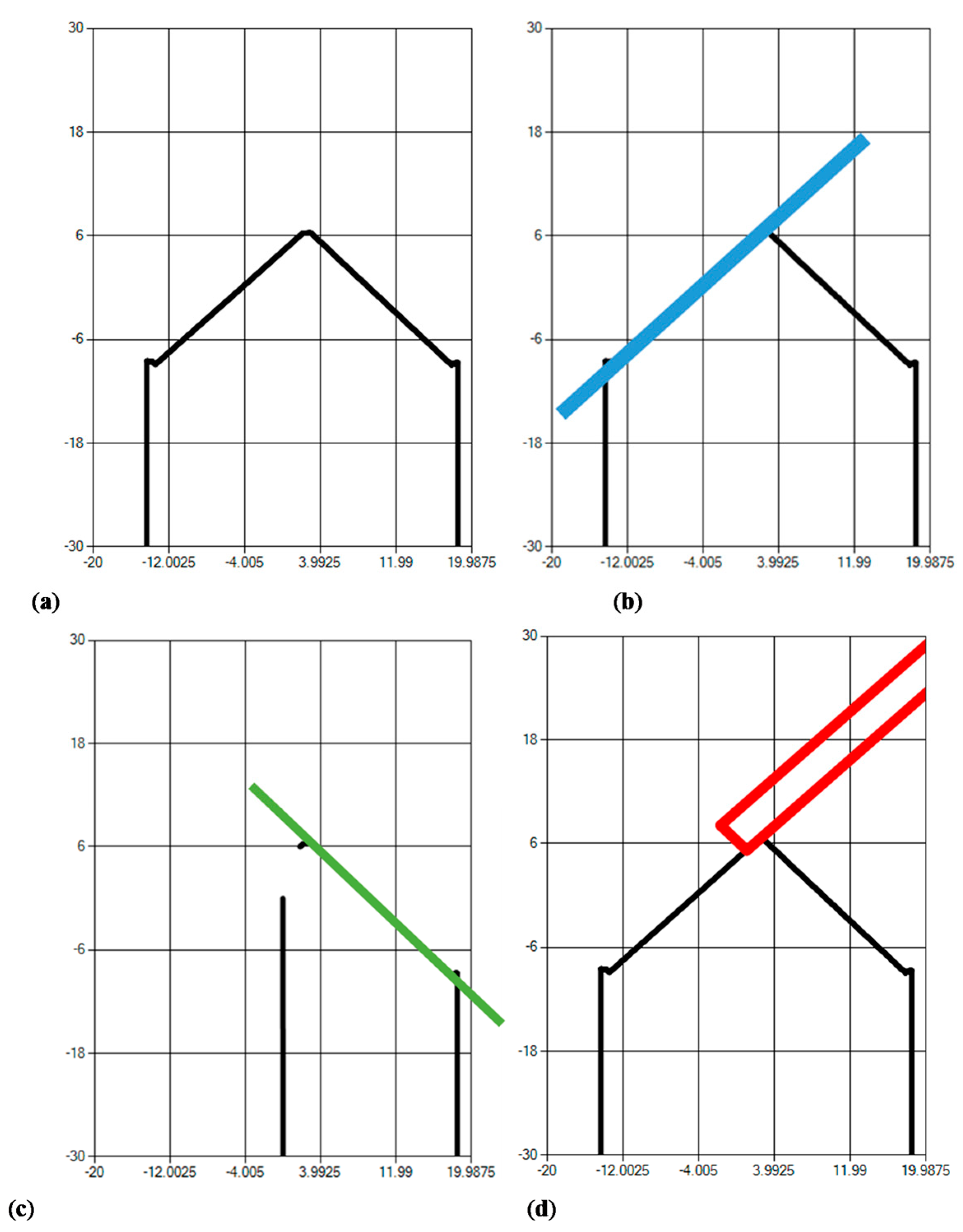
• Curve fitting is performed on the curve models obtained using the CAD cross-sectional contour characteristics. Using a fourth-order polynomial boundary curve equation as an example, the procedure is as follows:
  • The fourth-order polynomial model is expanded to $f\left(x\right)=a_0+a_{1}x+a_2{x}^2+a_3{x}^3+a_4{x}^4$.
  • If the contour curves are the curves of two different models, the contour points obtained from linear contour scanning are divided into head and tail sections for fitting; if the contour curves are the curves of a single model, the head and tail contour points obtained from linear contour scanning are substituted into the equations for fitting. The contour point dataset is $\left\{\left(x_1,y_1\right),\left(x_2,y_2\right),\left(x_3,y_3\right),\cdots ,\left(x_n,y_n\right)\right\}$
  • The error sum of squares of the contour data points for the fourth-order polynomial is calculated using $E\left(a_0,a_1,a_2,a_3,a_4\right)={\displaystyle \sum }_{i=1}^n{\left(y_i-\left(a_0+a_1{x}_i+a_2{x}_i{}^2+a_3{x}_i{}^3+a_4{x}_i{}^4\right)\right)}^2,$ where $a_0,a_1,a_2,a_3,$ and $a_4$ are unknown variables.
  • Curve fitting searches for a set of coefficients ($a_0,a_1,a_2,a_3,$ and $a_4$) that minimize errors; therefore, a first-order equation with a derivative of zero is used to determine the locations of the extrema, producing five linear equations. The simultaneous linear equations are solved to obtain the coefficients for the boundary contour curve equations (i.e., $a_0,a_1,a_2,a_3,$ and $a_4$).

    ▪

    Perform a partial derivation of E with respect to $a_0$ ($\frac{\partial }{\partial a_0}E\left(a_0,a_1,a_2,a_3,a_4\right)=0$) to solve for the position of the extreme value and obtain the first equation, which is expressed as follows: ${\displaystyle \sum }_{i=0}^n{a}_0+a_1{\displaystyle \sum }_{i=0}^n{x}_i+a_2{\displaystyle \sum }_{i=0}^n{x}_i{}^2+a_3{\displaystyle \sum }_{i=0}^n{x}_i{}^3+a_4{\displaystyle \sum }_{i=0}^n{x}_i{}^4={\displaystyle \sum }_{i=0}^n{y}_i$

    ▪

    Perform a partial derivation of E with respect to $a_1$ $(\frac{\partial }{\partial a_1}E\left(a_0,a_1,a_2,a_3,a_4\right)=0$) to solve for the position of the extreme value and obtain the second equation, which is expressed as follows: $a_0{\displaystyle \sum }_{i=0}^n{x}_i+a_1{\displaystyle \sum }_{i=0}^n{x}_i{}^2+a_2{\displaystyle \sum }_{i=0}^n{x}_i{}^3+a_3{\displaystyle \sum }_{i=0}^n{x}_i{}^4+a_4{\displaystyle \sum }_{i=0}^n{x}_i{}^5={\displaystyle \sum }_{i=0}^n{x}_i{y}_i$

    ▪

    Perform a partial derivation of E with respect to $a_2$ $(\frac{\partial }{\partial a_2}E\left(a_0,a_1,a_2,a_3,a_4\right)=0$) to solve for the position of the extreme value and obtain the third equation, which is expressed as follows: $a_0{\displaystyle \sum }_{i=0}^n{x}_i{}^2+a_1{\displaystyle \sum }_{i=0}^n{x}_i{}^3+a_2{\displaystyle \sum }_{i=0}^n{x}_i{}^4+a_3{\displaystyle \sum }_{i=0}^n{x}_i{}^5+a_4{\displaystyle \sum }_{i=0}^n{x}_i{}^6={\displaystyle \sum }_{i=0}^n{x}_i{}^2{y}_i$

    ▪

    Perform a partial derivation of E with respect to $a_3$ ($\frac{\partial }{\partial a_3}E\left(a_0,a_1,a_2,a_3,a_4\right)=0$) to solve for the position of the extreme value and obtain and the fourth equation, which is expressed as follows: $a_0{\displaystyle \sum }_{i=0}^n{x}_i{}^3+a_1{\displaystyle \sum }_{i=0}^n{x}_i{}^4+a_2{\displaystyle \sum }_{i=0}^n{x}_i{}^5+a_3{\displaystyle \sum }_{i=0}^n{x}_i{}^6+a_4{\displaystyle \sum }_{i=0}^n{x}_i{}^7={\displaystyle \sum }_{i=0}^n{x}_i{}^3{y}_i$

    ▪

    Perform a partial derivation of E with respect to $a_4$ ($\frac{\partial }{\partial a_4}E\left(a_0,a_1,a_2,a_3,a_4\right)=0$) to solve for the position of the extreme value and obtain the fifth equation, which is expressed as follows: $a_0{\displaystyle \sum }_{i=0}^n{x}_i{}^4+a_1{\displaystyle \sum }_{i=0}^n{x}_i{}^5+a_2{\displaystyle \sum }_{i=0}^n{x}_i{}^6+a_3{\displaystyle \sum }_{i=0}^n{x}_i{}^7+a_4{\displaystyle \sum }_{i=0}^n{x}_i{}^8={\displaystyle \sum }_{i=0}^n{x}_i{}^4{y}_i$

    ▪

    Solve the linear simultaneous equations, and obtain the coefficients of the contour boundary curve equations ($a_0,a_1,a_2,a_3, \mathrm{and} a_4$).

2.3. Detect Burrs and Generate Deburring Trajectories

The contour information obtained using the linear contour scanning sensors must be processed and undergo curve fitting to obtain the boundary contour equations and curves for the workpiece cross-sections. Thereafter, boundary contour equations are used to divide the space into two intervals to detect the burr distribution according to the generated deburring processing trajectories. The trajectory generation process is as follows:

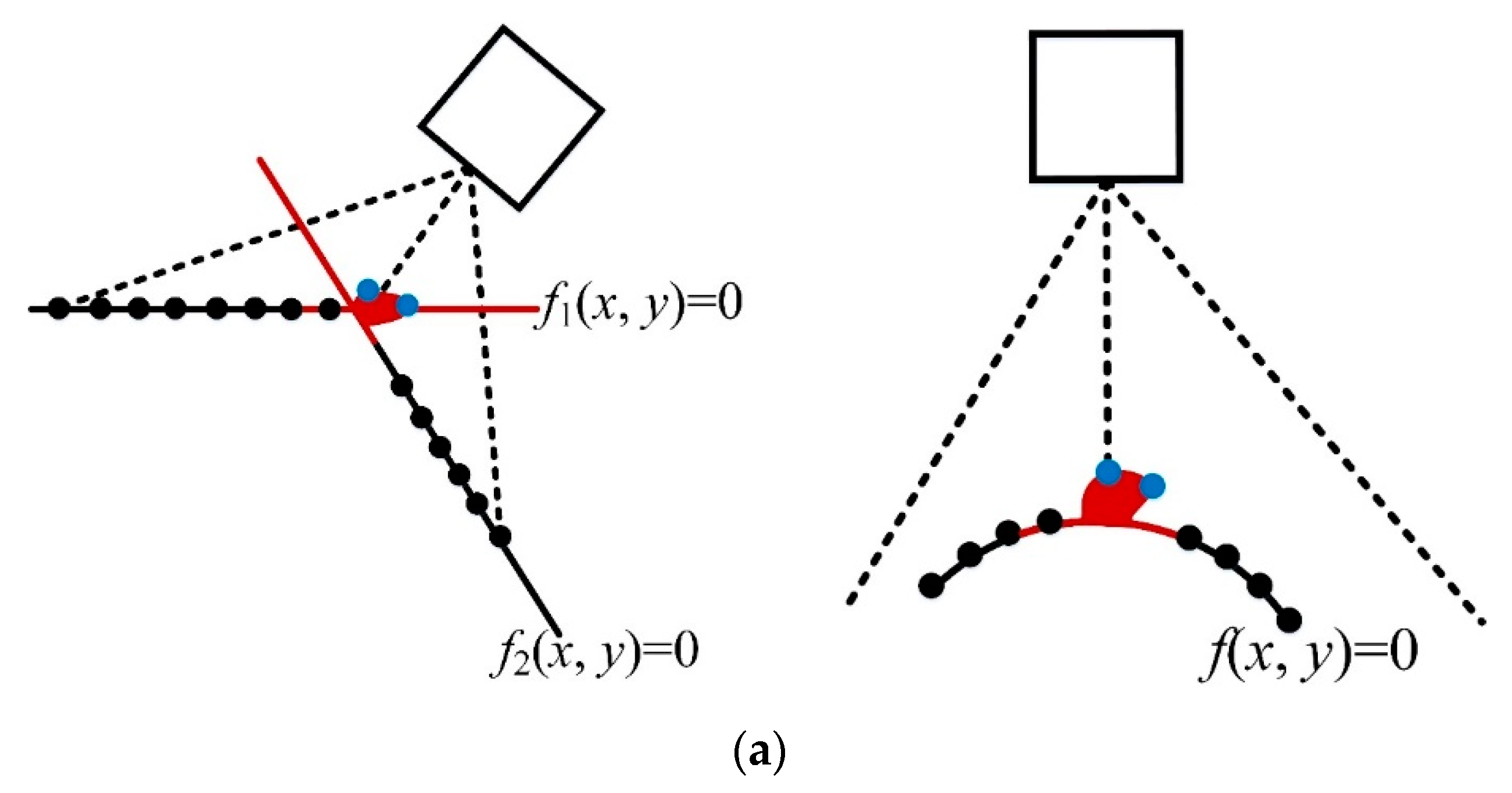
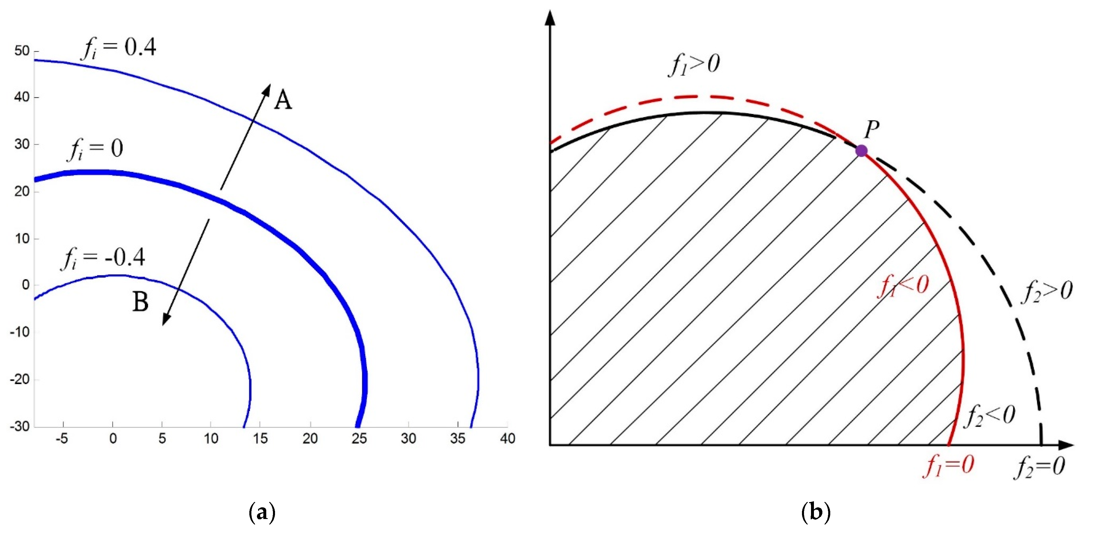
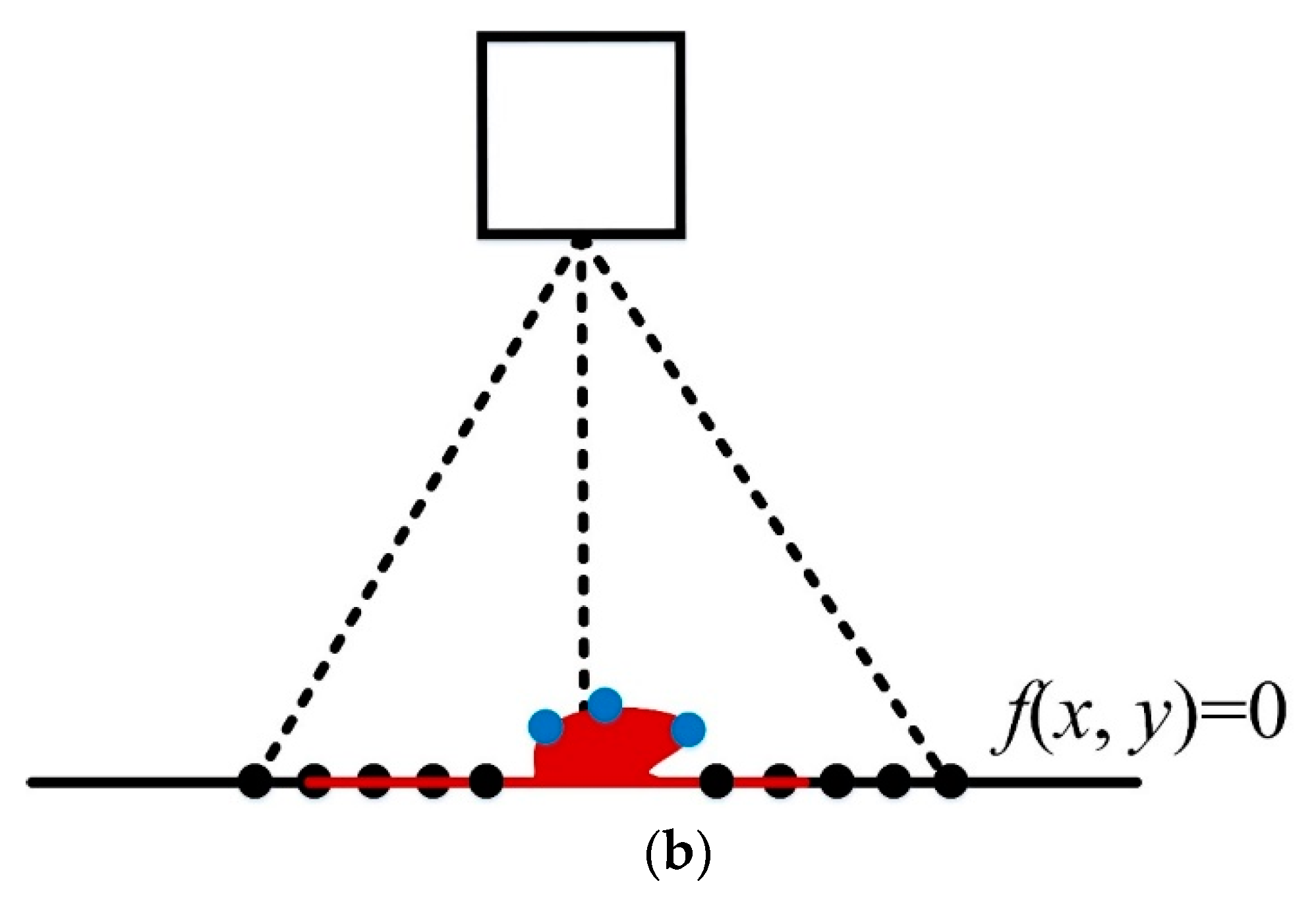
• The equation obtained through curve fitting is defined as the boundary contour curve equation $f_i\left(x,y\right)=0$, and the space is divided into two intervals (i.e., workpiece region A [the region on the same side as the sensor] and environmental region B [the region on the same side as the sensor]). Intervals A and B correspond to the positive and negative signs of equation function value $f_i$; therefore, to obtain the positive and negative signs of the functions corresponding to the equations in the two areas, the sensor coordinates are substituted to derive $f_i\left(x,y\right)=c$, which represents the positive and negative signs of the function values corresponding to the inadmissible interval. If the equation function value corresponding to the environmental area is <0, then $f_i=-f_i$, and all the equation function values corresponding to the workpiece intervals are ≤0 (Figure 5a). If the cross-sectional boundary contour curves are composed of different line segments, the intersection area where $f_i<0$ is the inner side of the workpiece cross-sectional contour (Figure 5b).
• The contour point information obtained from linear contour scanning is substituted into the equations. ε is the allowable boundary contour error, and its value is determined by sensor precision and the residual plot error values (Figure 6). If the value of any function $f_i\left(x,y\right)>\epsilon$, burrs are located at $\left(x,y\right)$.
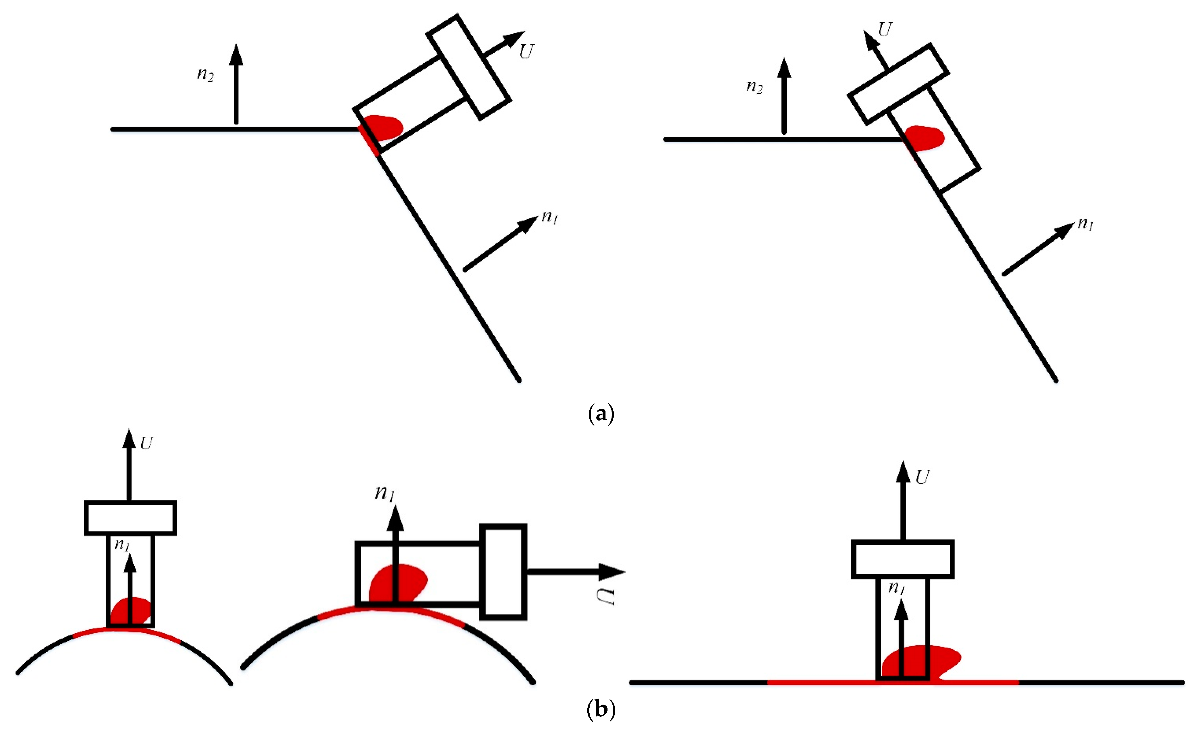
• Deburring trajectories are generated according to the contour data and burr detection results through the following procedure: (1) The bottom of the cutter is aligned with the contour curve, with the cutter’s U axis and curve normal vector facing in the same direction, to generate the deburring processing points and cutter direction. (2) The cutter axis is placed parallel to the direction of the contour, the center of the cutter is shifted in the direction of $n_1$ according to the cutter radius, and the direction of the contour is shifted by a specified amount (Figure 7).
• The robotic arm is moved forward to the deburring processing points to remove the burrs, and burr analyses and trajectory generation are performed for the next boundary contour. Once all the deburring regions have been scanned and processed, the deburring of the target workpiece is considered complete.

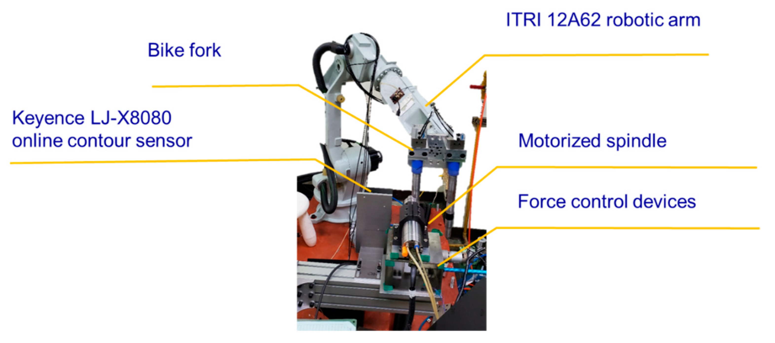
3. Verifying the Automatic Deburring System

To verify the feasibility of the method proposed in this study, the Industrial Technology Research Institute’s 12A62 robotic arm (which has a movement range of 1406 mm, a repeatability accuracy of 0.06 mm, and an absolute positioning precision of approximately 5 mm, according to the ISO9283 standard for laser trackers) was used to test the automatic deburring system. The method was applied to a bicycle fork processed through die casting. The dimensions of the robotic arm are presented in Figure 8. The system consisted of a Taiwan-made robotic arm controller, a Keyence LJ-X8080 online contour sensor (which had a measurement depth of 41 ± 20.5 mm, a width of 30–39 mm [depending on the depth], a repeatability accuracy of 0.5 μm, and a sampling frequency of 16 kHz), and a motorized spindle with ∅6 four-edge standard milling cutters (Figure 9).

To enable immediate deburring after scanning, the regions scanned by the contour scanning sensors were placed as close to the processing locations of the spindle milling cutters as possible. When the milling cutters moved to the burr locations after scanning, the laser contour scanning sensors were required to obtain the next cross-sectional contour information to determine the next processing trajectory point (Figure 10).

After the system was set up, the robotic arm controller and contour output controller were connected using network cables and the digital communication method. The robotic arm controller obtained contour information by using the API provided by the contour output controller. Once the contour information was obtained, adjustments were made using the hand–eye calibration method [23] and the spindle coordinate system correction method to determine the relative relationships among the contour sensors, spindle locations, and robotic arm coordinate system.

The deburring process started at the location where the contour scanning sensors could capture contour information. Once the contour information was obtained, the proposed method was used to analyze the burring region and generate processing trajectories. The burr locations were aligned with the spindle for deburring and to obtain the next cross-sectional contour for additional analyses. The proposed procedure enables continuous processing trajectory generation and complete deburring (Figure 11 and Figure 12).

Figure 12a shows the bicycle fork used for system verification. Figure 11 illustrates the cross-sectional data from Figure 12a that were obtained using laser contour scanning sensors. By applying the proposed method, the deburring trajectory could be generated for the subsequent deburring process. The result of the processing along the cross-sectional contour is displayed in Figure 12b.

The proposed method can be applied to deburr workpieces after molding as well as to deburr workpiece edges after cutting. Because the processed edges comprise two discontinuous line segments, the two segments must be fitted separately during curve fitting (Figure 13). All the contour information was first input into the linear equation to obtain the first line segment, and the interior point $m_i$ was removed from the contour points obtained by the sensors to generate a new contour point set. The second fitting was performed thereafter to obtain the mathematical equation for the second line segment. Finally, the two-line segment equations were used to obtain the focus locations, after which the processing trajectories were generated.

4. Conclusions

This study focused on the use of automatic deburring technology on multi-axis mechanisms for real-time, online deburring trajectory recognition. The proposed automatic deburring system may serve as a solution to certain robotic arm industry problems, especially those related to automated deburring. The contributions of this study are as follows:

• Regarding the automated equipment and systems integration technology required by the robotic industry, this study developed a model and automated technology for deburring using robotic arms, which may facilitate the integration between midstream and downstream supply chains, create complementary and clustering effects, and enhance the commercialized automated systems and relevant systems integration technology used by domestic firms.
• This study’s technological contributions will help the domestic robotics industry further improve and develop new applications for robotic arms and will facilitate the development of complete solutions to the industrial robotic arm and machine tool integration.
• The online deburring trajectory generation technology presented herein solves the problems encountered by domestic firms when using automated robotic arms (e.g., requiring a series of calibrations and compensations, generating trajectories only after using force control devices and offline programming software that can cost as much as NT$4.3 million, and facing costs and inefficiencies that may create an inability to satisfy industry demand).

The method proposed in this study captured workpiece cross-sectional contours online by using linear contour scanning sensors and adopted the RANSAC approach to identify burr locations and generate trajectories in real-time, thereby achieving automatic deburring processing. The method was tested using bicycle forks, and the results revealed that when the processing quality was maintained, work that originally took three to four people 8–12-h to complete was completed by one person in 30 min. In addition, the production cost was reduced by 70%. In the future, this method can be used by metal cutting and molding firms to minimize the time and costs required to integrate automatic deburring systems into their operations. The method can be integrated with smart mechanical system unit controllers in the future to solve problems related to project development and planning and can be used to build domestic controllers and smart processing systems to increase the market share and technological independence of domestically manufactured equipment.

References

1. International Federation of Robotics. World Robotics Report 2019; International Federation of Robotics: Frankfurt, Germany, 2019. [Google Scholar]
2. International Monetary Fund. World Economic Outlook; International Monetary Fund: Washington, DC, USA, 2019. [Google Scholar]
3. Wu, J.H.; Zhang, D.Q.; Jiang, C.; Han, X.; Li, Q. On reliability analysis method through rotational sparse grid nodes. Mech. Syst. Signal. Process 2021, 147, 107106. [Google Scholar] [CrossRef]
4. Zhao, Q.Q.; Guo, J.K.; Zhao, D.T.; Yu, D.W.; Hong, J. Time-dependent system kinematic reliability analysis for robotic manipulators. J. Mech. Des. 2021, 143, 041704. [Google Scholar] [CrossRef]
5. Wu, J.H.; Zhang, D.Q.; Liu, J.; Jia, X.Y.; Han, X. A computational framework of kinematic accuracy reliability analysis for industrial robots. Appl. Math. Model. 2020, 82, 189–216. [Google Scholar] [CrossRef]
6. Zhao, Q.Q.; Guo, J.K.; Hong, J. System kinematic reliability analysis for robotic manipulators under rectangular and spherical tolerant boundaries. J. Mech. Robot. 2021, 13, 011004. [Google Scholar] [CrossRef]
7. Gu, Y. Deburring Device including Visual Sensor and Force Sensor. U.S. Patent 9724801, 8 August 2017. [Google Scholar]
8. Kuss, A.; Drust, M.; Verl, A. Detection of workpiece shape deviations for tool path adaptation in robotic deburring systems, 49th CIRP. Procedia CIRP 2016, 57, 545–550. [Google Scholar] [CrossRef]
9. Leo, P.F.; Selvaraj, T. Vision assisted robotic deburring of edge burrs in cast parts. Procedia Eng. 2014, 97, 1906–1914. [Google Scholar]
10. Song, H.C.; Kim, B.S.; Song, J.B. Tool path generation based on matching between teaching points and CAD model for robotic deburring. In Proceedings of the 2012 IEEE/ASME International Conference on Advanced Intelligent Mechatronics, Kaohsiung, Taiwan, 11–14 July 2012; pp. 890–895. [Google Scholar]
11. Kosler, H.; Pavlovčič, U.; Jezeršek, M.; Možina, J. Adaptive robotic deburring of die-cast parts with position and orientation measurements using a 3D laser-triangulation sensor. J. Mechan. Eng. 2016, 62, 207–212. [Google Scholar] [CrossRef] [Green Version]
12. Lee, Z.C.; Bai, X.; Lin, C.S.; Wang, B.Y. A Kind of Robotic Deburring’s System and Burr Removing Method with Vision-Based Detection. CN106041948B, 13 June 2016. [Google Scholar]
13. Brogardh, T. System for Controlling the Position and Orientation of an Object in Dependence on Received Forces and Torques from a User. U.S. Patent 20090259412A1, 23 February 2006. [Google Scholar]
14. Hori, A.; Mori, K.; Fujita, T.; Sato, G.; Imagi, A.; Negishi, H. Processing Control Device, Machine Tool, and Processing Control Method. TWI667095B, 27 April 2017. [Google Scholar]
15. Zhang, K.; Chen, Y.X.; Zheng, J. A Kind of Automatic Identifying Method of Weld Joint Tracking Deviation and Cross-seam Type. CN108672988A, 19 October 2018. [Google Scholar]
16. Lovoi, P.A. Adaptive Tracking Vision and Guidance System. U.S. Patent 4907169A, 30 September 1987. [Google Scholar]
17. Neumann, K.E. Deburring Method. U.S. Patent 6155757A, 11 July 1996. [Google Scholar]
18. Gu, Y.; Satou, T. Deburring Apparatus. U.S. Patent 10478935B2, 8 December 2016. [Google Scholar]
19. Diaz Posada, J.R.; Kumar, S.; Kuss, A.; Schneider, U.; Drust, M.; Dietz, T.; Verl, A. Automatic programming and control for robotic deburring. In Proceedings of the ISR 2016: 47th International Symposium on Robotics, Munich, Germany, 5 September 2016. [Google Scholar]
20. Khalaj, O.; Jamshidi, M.; Saebnoori, E.; Masek, B.; Stadler, C.; Svoboda, J. Hybrid machine learning techniques and computational mechanics: Estimating the dynamic behavior of oxide precipitation hardened steel. IEEE Access 2021, 9, 156930–156946. [Google Scholar] [CrossRef]
21. Jamshidi, M.; Lalbakhsh, A.; Alibeigi, N.; Soheyli, M.; Oryani, B.; Rabbani, N. Socialization of industrial robots: An innovative solution to improve productivity. In Proceedings of the 2018 IEEE 9th Annual Information Technology, Electronics and Mobile Communication Conference (IEMCON), Vancouver, BC, Canada, 17 January 2019. [Google Scholar] [CrossRef]
22. Fischler, M.A.; Bolles, R.C. Random sample consensus: A paradigm for model fitting with applications to image analysis and automated cartography. Comm. ACM 1981, 24, 381–395. [Google Scholar] [CrossRef]
23. Li, J.; Chen, M.; Jin, X.; Chen, Y.; Dai, Z.; Ou, Z.; Tang, Q. Calibration of a multiple axes 3-D laser scanning system consisting of robot, portable laser scanner and turntable. Optik 2011, 122, 324–329. [Google Scholar] [CrossRef]
Figure 1. 3D online deburring trajectory generation process.
Applsci 12 04852 g001
Figure 2. Deburring regions: (a) processed edges, (b) parting lines, and (c) gates/risers.
Applsci 12 04852 g002
Figure 3. Residual plot analyses: (a,b) nonconstant residuals, and (c) unsuitable model.
Applsci 12 04852 g003
Figure 4. Burr detection system: contour scans of burrs on (a) processed edge and (b) parting lines/risers.
Applsci 12 04852 g004
Figure 5. External contour region recognition method. (a) Workpiece region and environmental region. (b) Workpiece cross−sectional contour.
Applsci 12 04852 g005
Figure 6. Automatic burr detection. (a) contour fitting of processed edge. (b) contour fitting of parting lines/risers.
Applsci 12 04852 g006aApplsci 12 04852 g006b
Figure 7. Deburring trajectory generation. (a) workpiece edges. (b) parting lines/risers.
Applsci 12 04852 g007
Figure 8. Industrial Technology Research Institute 12A62 robotic arm dimensions.
Applsci 12 04852 g008
Figure 9. Verifying the automatic deburring system.
Applsci 12 04852 g009
Figure 10. Relative relationship between contour scanning and spindle location.
Applsci 12 04852 g010
Figure 11. Cross−sectional contour information of bicycle fork (red box is the schematic of deburring tool): (a) contour information and (b) cutter trajectory.
Applsci 12 04852 g011
Figure 12. Bicycle fork (a) before and (b) after processing.
Applsci 12 04852 g012
Figure 13. Cross−sectional contour information of the workpiece cutting edges (the blue and green lines shows the contour fitting result, and the red box is the schematic of deburring tool): (a) contour information, (b) fitting of first line segment, (c) fitting of second line segment, and (d) cutter trajectory.
Applsci 12 04852 g013
Publisher’s Note: MDPI stays neutral with regard to jurisdictional claims in published maps and institutional affiliations.