The Investigation of a New End Wall Contouring Method for Axial Compressors

Abstract

To further control corner separation in high-load axial compressors, this study proposes a new end wall contouring method. It defines multiple standard “surface units” with particular flow control effects and then applies a linear combination, finally forming the geometry of the end wall surface. Based on design experiences, three different end wall contouring cases are generated and calculated on a high-load compressor cascade in the first step. The results show that the new method achieves a clear and intuitive influence on the end wall geometry, with a proper number of design variables, and can effectively combine variables with the development of secondary flow. In the second step, the new method was applied to an axial compressor, with an improvement in the design variables. Although the end wall contouring only improved the efficiency of the compressor stage on the right part of its operating map, the experimental results of the flow field show that the corner separation and end wall loss are suppressed at multiple inflow conditions. The results thus verified the practical effect of the newly developed end wall contouring method.

1. Introduction

Compressors of the turbine engine have been designed with higher loads in recent years. As a result, the high pressure gradient across the blade channel increases the three-dimensional effect of the end wall region. The resultant corner separation becomes a problem for the efficiency and stability of compressors. Therefore, the high-load compressor commonly requires flow control techniques to improve its performance.

As a passive flow control technique in turbomachinery, end wall contouring was first proposed in turbines and then applied in axial compressors in past decades [1]. The basic principle of end wall contouring is to alter the local static pressure field by generating small concave and convex on the end wall surface. The variation of the pressure field then affects the secondary flow motion, finally helping to relieve the corner separation. Compared to the well-known three-dimensional sweep and lean, end wall contouring has little effect on the stacking law of the blade and barely alters the blade loading. In recent years, numerous numerical and experimental studies have confirmed its significant effect in suppressing corner separation and improving the performance of compressors [2,3,4,5,6].

The end wall contouring design method broadly comprises two categories in published studies. One is the empirical method. The design process uses the analytical formula or manual adjustment to create the geometry of the entire end wall, thereby controlling the overall end wall secondary flow. According to the Bernoulli equation, a convex surface forms a convergent channel locally and depressurize the flow, and a concave surface has the opposite effect. Thus, a downslope from the PS to the SS (called DPS for short) will reduce the cross-passage pressure gradient and suppress the end wall secondary flow. Hu’s research [7] generated the DPS with a sine function to suppress the secondary flow, finally reducing the corner separation and increasing the peak efficiency by 0.45%. The DPS is also found in a much more recent study of a compressor cascade by Cao [8], where the end wall contouring similarly reduced 18% of the total pressure loss. An afterward study by Meng et al. [2] combined the end wall contouring with the SS corner profiling, proving that even using a straight-shaped DPS would suppress the end wall second flow and benefit the separation control. Note that the DPS is not the only contouring rule for loss control. The exception is in Harvey’s research [9], where the end wall contouring is manually constructed with an upslope from PS to the SS (called UPS for short), thus accelerating the end wall secondary flow to pre-mix with the accumulated low-energy fluid. Finally, the spanwise distribution of the loss coefficient was reduced by up to 7% relative to the original case. Therefore, it is hard to say whether decelerating or accelerating the end wall secondary flow would be more effective in separation control.

The other end wall contouring method, i.e., the optimization method, shows more diversity than the empirical method. The parametric end wall surface is traditionally constructed using a lofted surface over dozens of uniformly distributed free control points, thus enabling highly flexible variation to work out the best end wall contouring in the design space. According to the optimization results, some research found weakening of the end wall secondary flow to be most effective in controlling corner separation [10,11,12,13,14,15]. However, the results are different from the DPS in the empirical method. The end wall might have a downslope, but it is more likely a localized surface near the SS [10] or from the center of the blade channel [11] rather than a full-range structure. Some even find that the optimum end wall generates a streamwise groove, thus inducing a contour vortex to the passage vortex and deflecting the end wall secondary flow before it reaches the SS corner [12,13,14,15]. The most frequently reported effective flow control is the acceleration of cross and climbing flow in the SS corner [3,16,17,18,19]. The optimization results show their diversity even with a common feature. In Harvey’s study [16], the acceleration of the end wall secondary flow is caused by a localized fillet-like upslope surface to the SS corner. Varpe’s research [17] shows a similar feature but a different position and area. Moreover, in the studies of Zhang [11], Reising [18], Lepot [19], and Ma [3], the upslope surfaces in the SS corner are all connected with concave surfaces in the peripheral regions and thus able to enhance the end wall secondary flow further.

Table 1. Effect of different flow control techniques on turbomachineries.

Flow Control Techniques	Application	Researchers	Improvement of Efficiency
fillet in the SS corner	compressor rotor 67	Ji [21]	0.3%~0.5% (different rotating speed)
three-dimensional blading	a compressor rotor	Mahmood [22]	0.7% (peak efficiency)
three-dimensional blading	compressor stage 35	Cheng [23]	0.53% (peak efficiency)
end wall contouring	a compressor stage	Sun [24]	0.2%~0.3% (best improvement)
end wall contouring	Trent 500 HP turbine	Brennan [25]	0.4% (peak efficiency)
end wall contouring	a compressor rotor	Hu [7]	0.45% (peak efficiency)

compares the general effect of the flow control technique on the compressors or turbines in some typical studies. There are two studies of end wall contouring included, showing that the improvement of efficiency reaches 0.3~0.5%, which is comparable to those of the three-dimensional blading. It is worth noting that the above summary only describes the general features and effects of the end wall surface. More details, including the location, intensity, and area of the effect of end wall contouring, are not mentioned, but they may change from one case to another. According to some more recent research, the diversity of the optimum results should be associated with the variation of incidence of inflow [4], the solidity of the blade passage [5], or even the thickness and skewness of the inflow boundary layer [6,20]. Therefore, the results actually indicate that the parametric surface of end wall contouring should, at the very least, affect the end wall secondary flow from more than one position to make itself more effective. This is what the traditional empirical method lacks. In comparison, the optimization method seems more reliable, but there are still problems during application. Except for its time-consuming simulation during the design iterations, the flow control rules of a particular optimal end wall contouring are commonly not widely applicable. Thus, the design rules of the end wall contouring are difficult to establish. With the above problems, this study developed a new end wall contouring method for compressors, which shows improvement in the following aspects:

• The number of parameters is limited to an appropriate level, making the method easy to use. The parameters have a clear and intuitive influence on the end wall geometry and the intent of flow control.
• The design space is large enough to accommodate suitable aerodynamic end wall shapes for a wide range of compressor cases.
• The new method can take into account the control of multiple local secondary flows while facilitating the integration of previous design experience.

The following paragraph will introduce the new end wall contouring method in Section 2, followed by a numerical investigation of a linear cascade in Section 3. An experiment on a compressor stator was carried out to verify the new method, and the results are presented in Section 4. Finally, Section 5 concludes the paper.

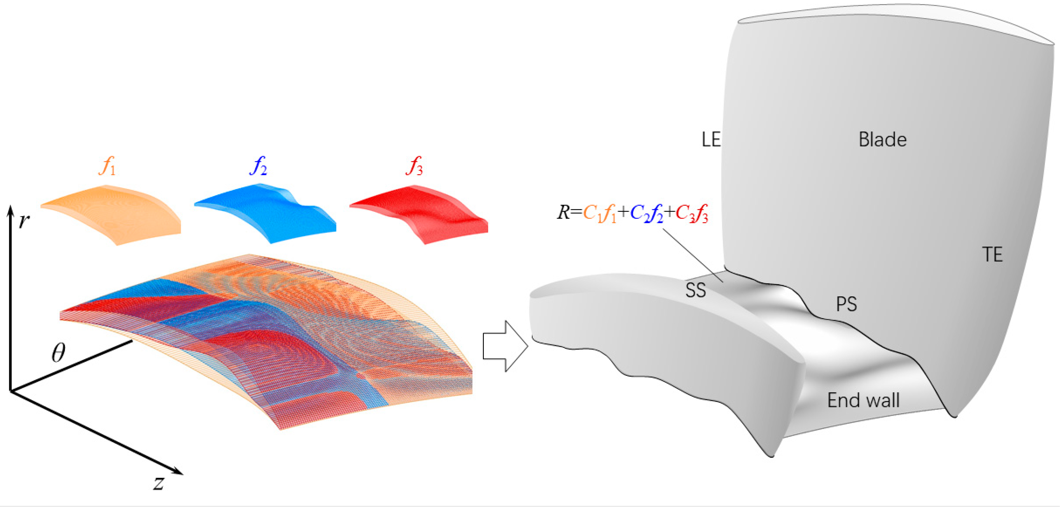
2. New End Wall Contouring Method

To control the second flow in multiple local areas, the main idea of the new end wall contouring method is to generate multiple “units” with particular effects for the secondary flow. Then, we apply a weighted superposition to these units, as shown in Figure 1, to obtain a comprehensive flow control effect. The parametric equation for the end wall surface can be written as

$$R(z,\theta )={\displaystyle \sum _{i=1}^n{C}_i{f}_i(z,\theta )}$$

(1)

Each f_i(z, θ) term of Equation (1) is a smooth and continuous function defined on the end wall z-θ plane, meaning the spanwise coordinate (r) of an individual end wall contouring unit. Herein, they are named unit functions for brevity in the following statement. We defined C_i as the corresponding weight factor. The overall shape of end wall contouring will be dependent on each unit function and the value of their weight factors. Considering the previous research in the Introduction, we propose two types of end wall contouring units.

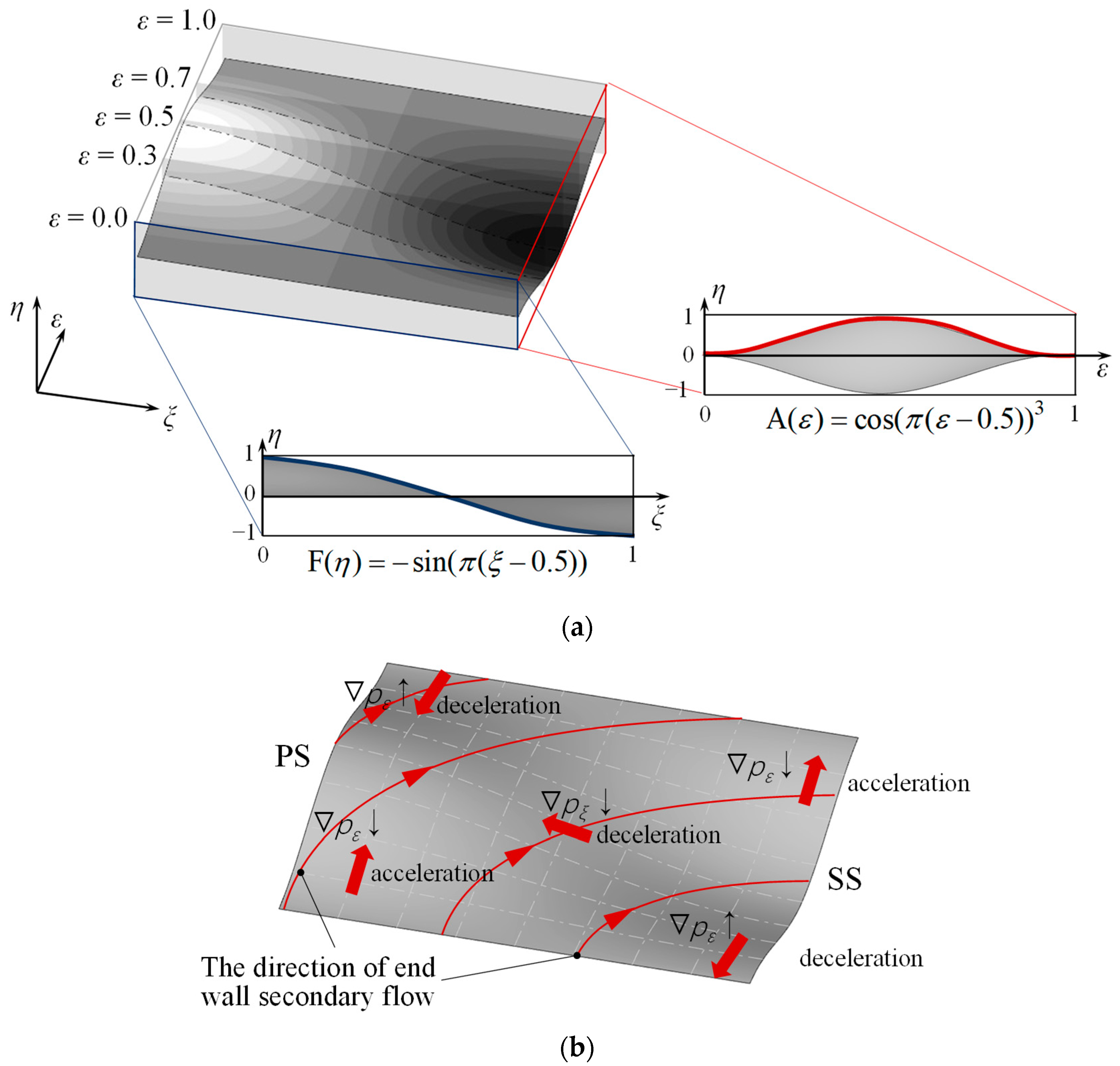
2.1. The Definition of the End Wall Contouring Units

(1)

The full-area unit

The first type of end wall contouring unit is designed to accelerate or decelerate the cross-passage secondary flow over the end wall region. It is termed “full-area unit” for brevity. The definition is sketched in Figure 2. For the convenience of presentation, Figure 2a maps the z-θ end wall surface of the blade channel to a dimensionless 1 × 1 standard space and sets η, ξ, and ε to represent the spanwise, circumferential, and streamwise directions of the compressor channel. ε = 0 and ε = 1 represent the leading edge (LE) and trailing edge (TE) lines; ξ = 0 and ξ = 1 represent the PS and SS. Then, the control equations of the full-area unit can be expressed as

$$\mathrm{f}(\epsilon ,\xi )=\mathrm{A}(\epsilon )\mathrm{F}(\xi )=-\cos {(\pi (\epsilon -0.5))}^3\sin (\pi (\xi -0.5))$$

(2)

Note the streamwise function, i.e., A(ε) = cos(π(ε − 0.5))³ acts as the amplitude of the transverse function F(ξ) = −sin(π(ξ − 0.5)), and the maximum value of A(ε) locates at ε = 0.5. To further smooth the surface, we selected five axial sections (transparent sections labeled from S1 to S5 in Figure 2) at the streamwise position of ε = 0, 0.3, 0.5, 0.7, and 1 in the full-area unit to construct the lofting surface. Considering that there are only five sections, the interpolation of the surface uses the cubic spline to ensure it accurately gets through all the sections, finally forming the geometry for the full-area unit.

Consider that when the full-area unit is mapped to the actual end wall of the axial flow compressor, the shape of the surface causes the pressure side of the blade channel to sink and the suction side to rise, with the maximum slope at the 0.5 axial chord length (c_a) position. Figure 2b thus illustrates the possible variation of end wall flow according to the Bernoulli effect. In the circumferential direction, the full-area unit generates an upslope surface from the SS to the PS, just as in previous research [7,8]. So, the transverse pressure gradient (∇p_ξ) will decrease, and the cross-passage secondary flow will decelerate in the entire area. There are some side effects. On the suction side of the end wall, the variation of the streamwise pressure gradient (∇p_ε) will stay positive from the LE to the mid-chord and then negative till the TE. Therefore, the streamwise component of end wall flow will decelerate in the front half and then accelerate in the rear half. On the pressure side of the end wall, all side effects are contrary to the suction side. It should also be noted that when applied to an actual compressor, all the above flow control, including its impact on the cross-passage secondary flow and the side effects, may turn in the opposite direction when the weight factor is less than zero.

(2)

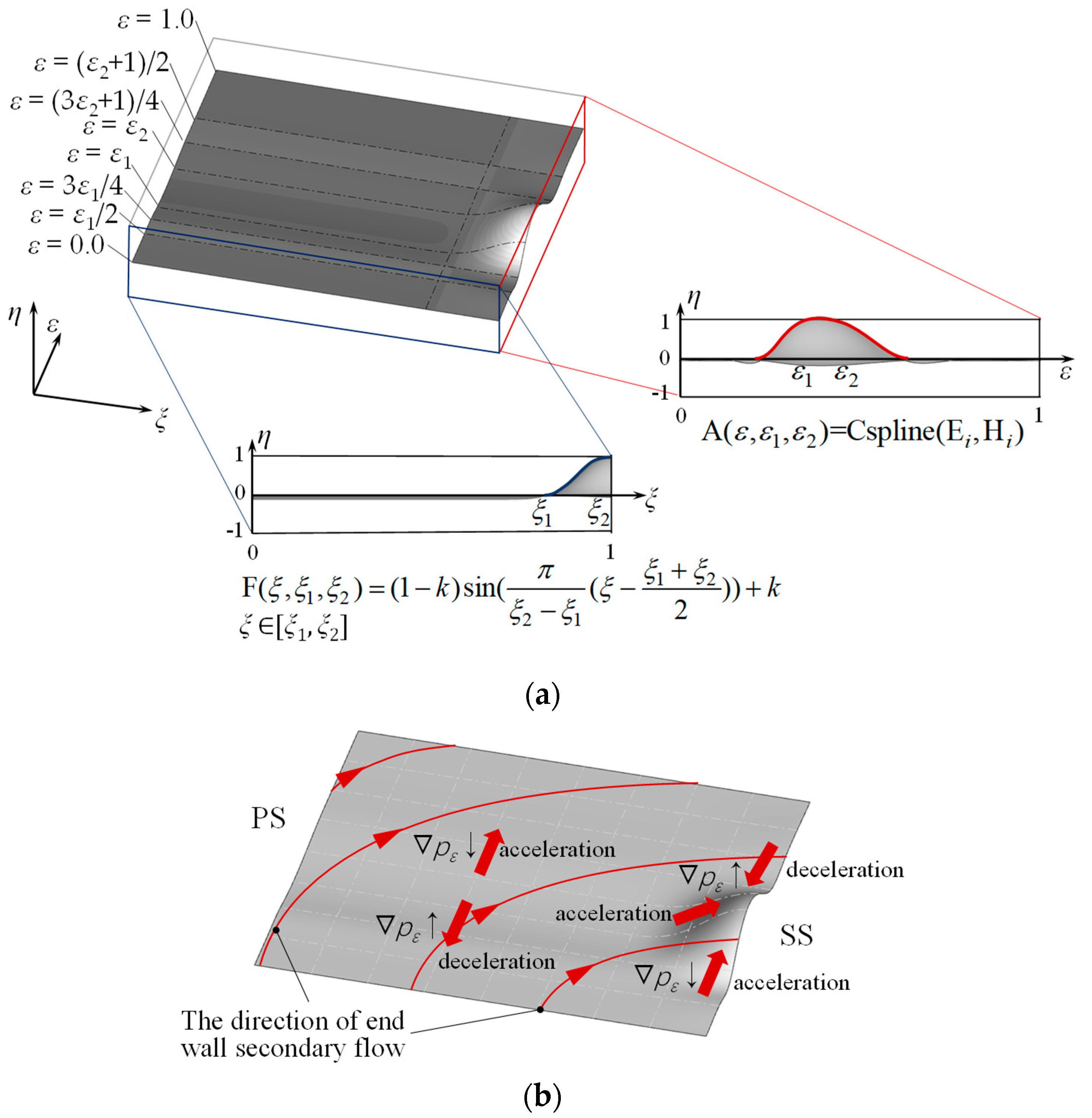
The localized unit

The second type of end wall contouring unit is defined to facilitate the secondary flow control in one or more particular local areas in the blade channel. It is termed the “localized unit” for brevity. The definition of this end wall contouring unit is shown in Figure 3a. Different from the full-area unit, the streamwise starting and ending positions ε₁, ε₂, and circumferential starting and ending positions ξ₁, ξ₂ in the localized unit are all free parameters. Varying these parameters will change the shape of the localized unit.

The parametric equation of the localized unit is

$$\mathrm{f}(\epsilon ,\xi )=(\mathrm{F}(\xi ,{\xi }_1,{\xi }_2)+k)\mathrm{A}(\epsilon ,{\epsilon }_1,{\epsilon }_2)$$

(3)

where

$$\mathrm{A}(\epsilon ,{\epsilon }_1,{\epsilon }_2)=\mathrm{Cspline}({{\rm E}}_i,H_i)$$

(4)

and

$$\mathrm{F}(\xi ,{\xi }_1,{\xi }_2)=\{\begin{array}{l}2k-1, \xi <{\xi }_1\\ (1-k)\sin (\frac{\pi }{{\xi }_2-{\xi }_1}(\xi -\frac{{\xi }_1+{\xi }_2}{2}))+k, {\xi }_1<\xi <{\xi }_2\\ 1, \xi >{\xi }_2\end{array}$$

(5)

The function of A(ε, ε₁, ε₂) of Equation (4) represents a cubic spline interpolation over eight control points and defines the amplitude distribution in the streamwise direction. The eight points are {Ε_i, H_i} = {(0, 0), (ε₁/2, 0), (3ε₁/4, 0), (ε₁, 1), (ε₂, 1), ((3ε₂ + 1)/4, 0), ((ε₂ + 1)/2, 0), (1, 0)}. The factor k is the zeroing factor. It is defined as

$$k=k|{\displaystyle \underset{{\xi }_1}{\overset{{\xi }_2}{\int }}\mathrm{F}(\xi ,{\xi }_1,{\xi }_2)=0}$$

(6)

Thus, k is able to make F(ξ) integrate to 0 on the transverse region of ξ ∈ [0, 1], thus ensuring that the cross-sectional area of the blade channel does not change.

Figure 3b shows the possible variation of the pressure field and the end wall flow when applying a localized unit in the end wall contouring. If C_i > 0, the end wall surface would warp up and create an upslope from ξ₁ to ξ₂. Thus, the transverse pressure gradient within {ξ ∈ [ξ₁, ξ₂] ∩ ε ∈ [ε₁, ε₂]} will increase, thus accelerating the cross-passage secondary flow locally. The side effects are similar to the full-area unit. On the suction side of the profiling region, the variation of ∇p_ε will accelerate the streamwise end wall flow in the upstream region and decelerate it in the downstream area. On the pressure side, the side effects become the opposite. As in the full-area unit, all the flow control may turn to the opposite direction when C_i < 0.

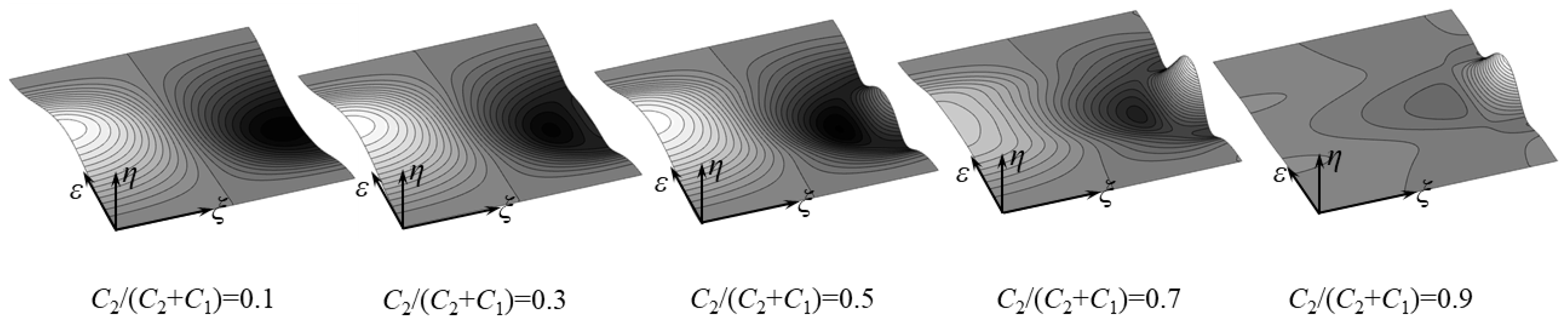
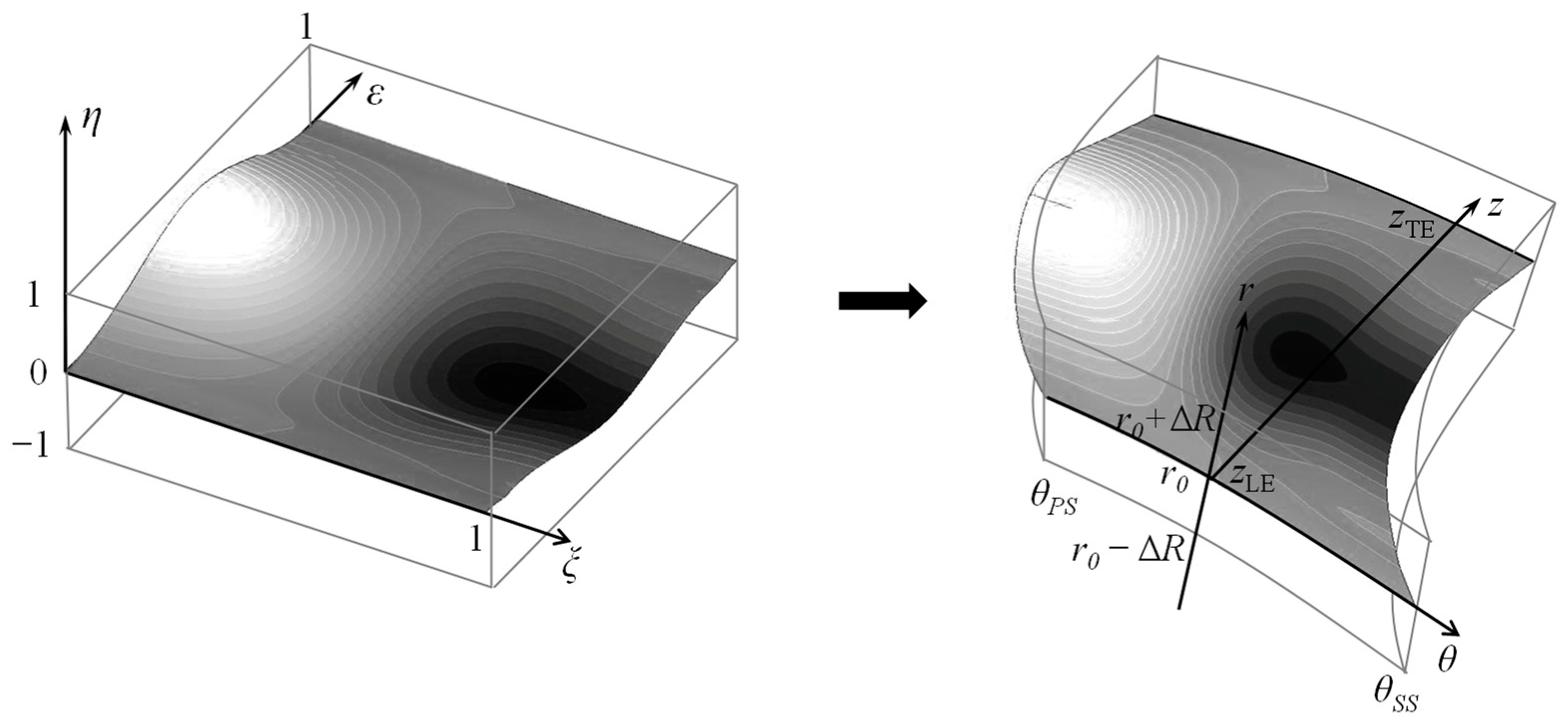
2.2. Generating End Wall Contouring in the Standard Space

The above end wall contouring units are combined according to Equation (1) to obtain geometry within the standard space. Note that each of the above units would affect end wall secondary flow in a particular region. Thus, the physical meaning of combining them as Equation (1) is to superimpose their effects, finally obtaining an end wall contouring with a comprehensive control effect on the end wall secondary flow. Supposing an end wall contouring includes a total of n units (labeled as f₁ to f_n), i.e.,

$$H=C_1{\mathrm{f}}_1+C_2{\mathrm{f}}_2+C_3{\mathrm{f}}_3\dots +C_n{\mathrm{f}}_n$$

(7)

The weight factor C_i would represent how much the ith unit affects the final control force on the end wall secondary flow.

Figure 4 illustrates an end wall surface consisting of a full-area unit and a localized unit as an example. The former is designed to suppress the cross trend of secondary flow over the end wall range, while the latter is intended to promote the cross trend of secondary flow in the SS corner region. As can be seen from the figure: the changes induced by adjusting the C₁ and C₂ are significant. When C₂/(C₁ + C₂) changes from 0.1 to 0.9, the overall slope of the surface from SS to PS gradually weakens, and the local shape along the SS corner becomes more and more prominent. Although the linear combination of the above two end wall contouring units does not mean their flow control would have a linear combination, it is known from the final end wall surface that the effect of the localized unit on the end wall flow near the SS corner gradually increases with the value of C₂/C₁.

2.3. Generating End Wall Contouring for the Actual Compressor

After obtaining the end wall contouring in the standard space of {(ε, ξ, η)| ε ∈ [0, 1], ξ ∈ [0, 1], η ∈ [−1, 1]}, the shape of the end wall contouring can be mapped directly to the three-dimensional end wall region of the axial compressor according to their spatial correspondence.

As shown in Figure 5, the coordinate system of the compressor end wall region is (r, θ, z). r₀ represents the radius of the baseline end wall surface; z_LE and z_TE represent the LE and TE axial coordinates; θ_PS and θ_SS represent the circumferential coordinates of the PS and the SS. Here, we correspond the end wall’s LE and TE to ε = 0 and ε = 1 and the SS and PS that form the blade channel to ξ = 0 and ξ = 1, and we limit the waviness of the actual end wall contouring within ±ΔR. Then, the end wall contouring in the standard space can be mapped to the actual axial compressor through

$$\{\begin{array}{l}r=\eta \Delta R(z)+r_0(z)\\ z=\epsilon (z_{\mathrm{TE}}-z_{\mathrm{LE}})+z_{\mathrm{LE}}\\ \theta =\xi ({\theta }_{\mathrm{SS}}(z)-{\theta }_{\mathrm{PS}}(z))+{\theta }_{\mathrm{PS}}(z)\end{array}$$

(8)

The above section discusses the definition and implementation process of this new end wall contouring method. Note that the new method can theoretically create arbitrary shapes by combining an infinite number of end wall contouring units. However, some preliminary studies indicate that combining one full-area unit and two localized units will usually be sufficient to control the corner separation. So, the new method generally requires less than 12 parameters for all the design processes.

3. Application in a High-Load Compressor Cascade

To evaluate the performance of the new end wall contouring method, it was first applied on a compressor cascade to see how it controls the corner separation.

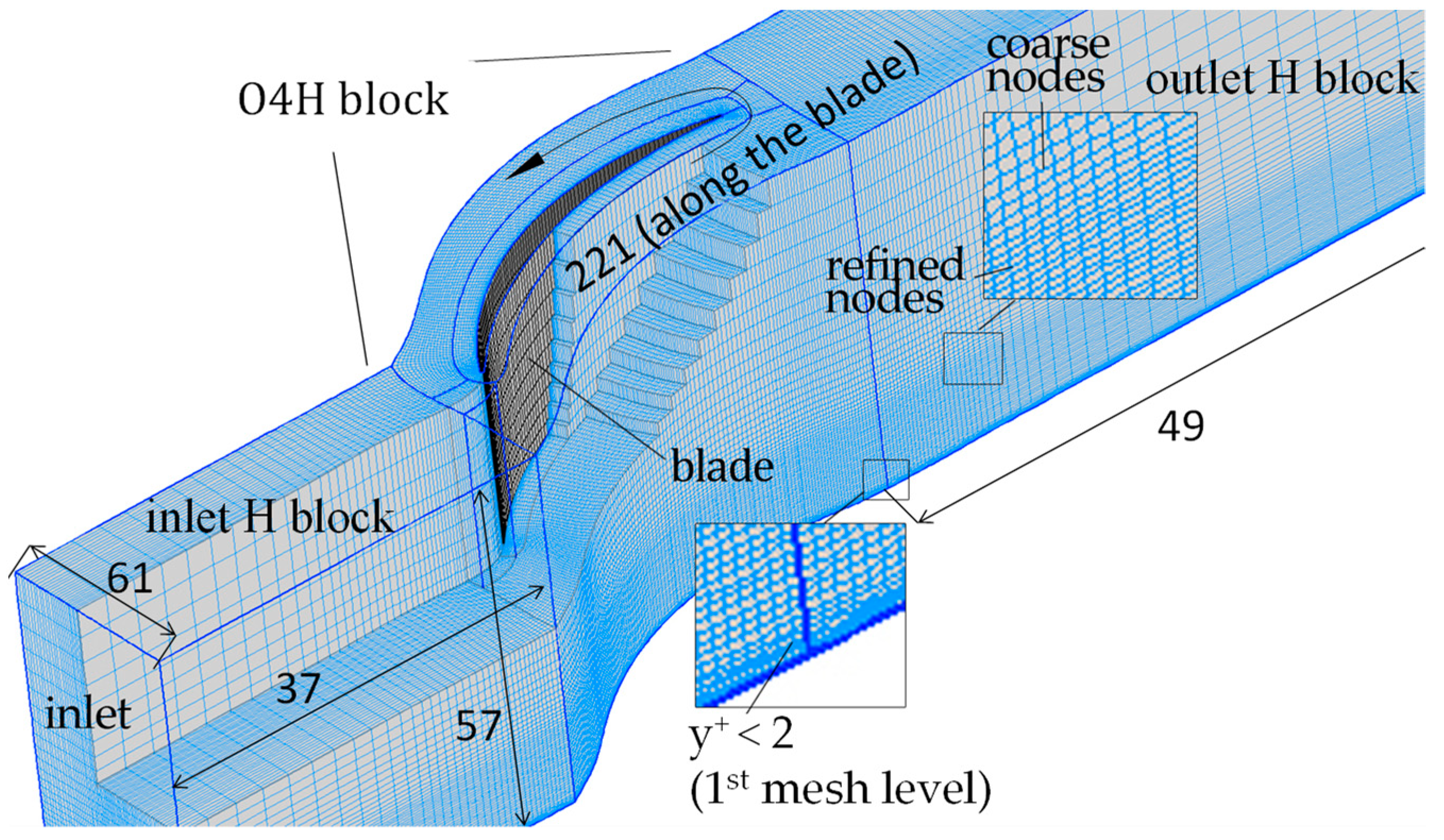
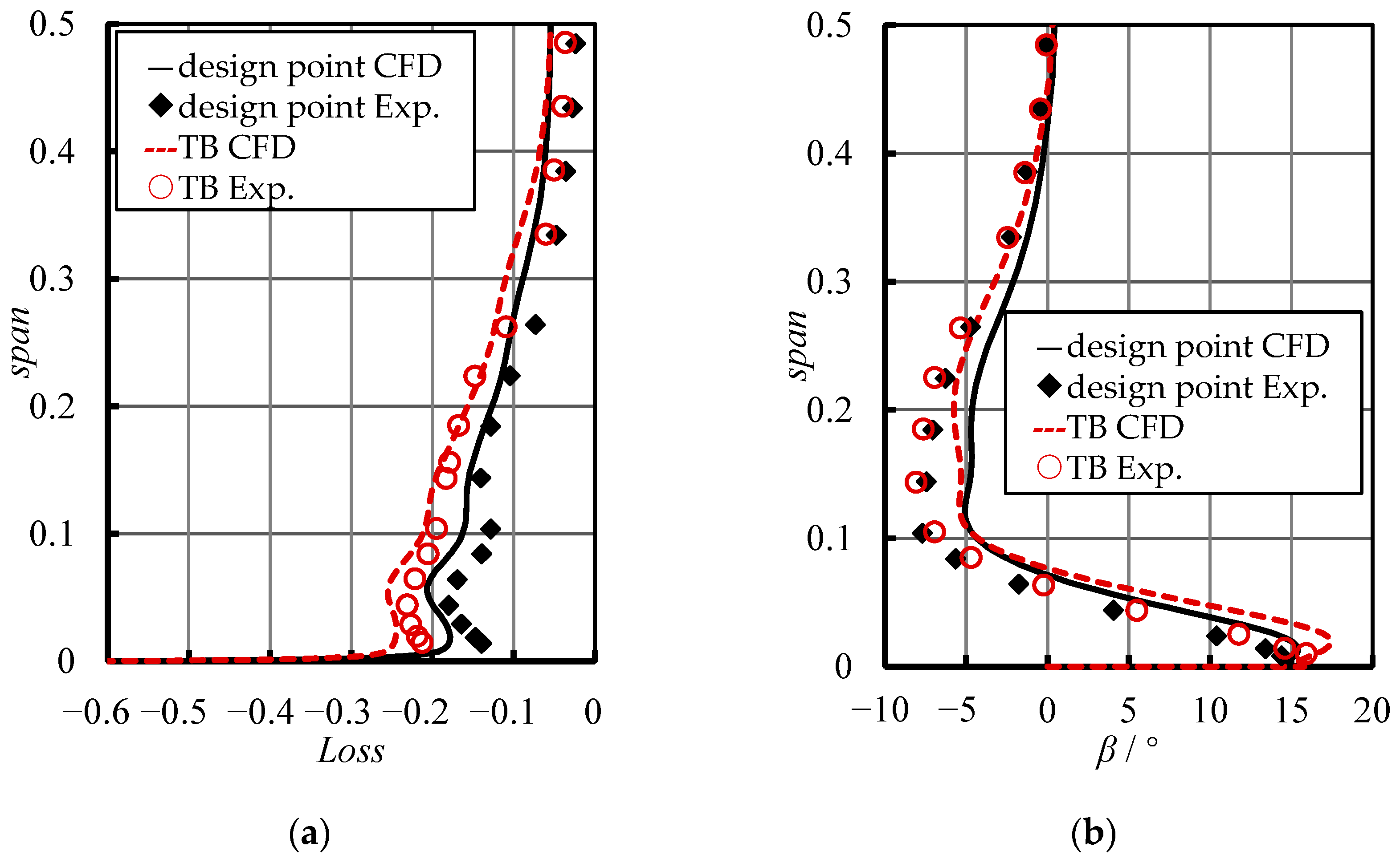
3.1. The Baseline Cascade and CFD Method

The research object is a high-load linear compressor cascade with a designed flow turning angle of 52°. The aspect ratio of the cascade is 2.0, and the solidity exceeds 2.1. There are detailed experimental studies that have been carried out on this cascade [26,27], showing that severe corner separation arises in this cascade even under the design incidence (i = −1°), and it will develop to corner stall when i exceeds 7°. Thus, the working point with i = +7° is named the near-stall (NS) point for brevity.

The computational domain of the cascade only includes a half-span region of the cascade. Figure 6 provides an overview of the computational mesh. The inlet and outlet passages both use long extended “H” blocks. The blade-to-blade flow surface employs refined nodes in the center with the “O4H” topology to achieve higher orthogonality. The number of nodes in some critical sections are also presented. The computational domain extended to 1.2 times the axial chord (C_a) upstream of the LE, where the inlet velocity is taken during the experiment, and to 2.0 C_a downstream of the TE for the uniformity of the outflow parameter. The mesh in the boundary layer region upon the blade surface and the end wall is further refined for accuracy in calculating the corner separation. The growth rate of mesh from the solid wall to the flow field is less than 1.1, and the y⁺ is less than two at the first level upon the solid wall. The boundary condition is given according to the experimental results. The inlet boundary defines the static temperature and the inflow velocity. The thickness of the inlet boundary layer is about 12.5%span. The outlet boundary defines a uniform static pressure.

The flow field of the cascade is regarded as compressible and full-turbulent. The Re for the current cascade is 1.4 × 10⁵.

Table 2. CFD settings for the inflow condition of the cascade.

Inlet Conditions	Values
static temperature	288.15 K
velocity of mainflow	26.5 m/s
thickness of inlet boundary layer	12.5%span
turbulent intensity	0.3%

provides details of the inflow condition. It is calculated with Numeca Fine/Turbo by solving the compressible steady Reynolds-averaged Navier–Stokes (RANS) equations with the k-ω turbulence model. The spatial discretization scheme uses the second-order central scheme. The convergence criterion was set to a value of 1 × 10⁻⁶ for the RMS residual values. Local time stepping techniques were applied to speed-up convergence.

All the above CFD settings are the same as previous numerical studies on this cascade [4], in which the CFD results were validated using the experimental outflow parameter and the oil-flow test on the SS and end wall surface. A grid convergence study was also applied, showing that a total of 0.75 million grid nodes is sufficient. Here, we offer only the validation of outflow loss coefficient (Loss) and flow angle (β) under the design working condition (i = −1°), as in Figure 7. The horizontal axis shows the loss coefficient, defined as

$$Loss=\frac{P^{*}-P^{*}{}_{\mathrm{in}}}{P^{*}{}_{\mathrm{in}}-P_{\mathrm{in}}}$$

(9)

where P*_in and P_in represent the inlet total pressure and static pressure in the mid-span position. The vertical axis means spanwise position normalized using the height of the blade. The result labeled “TB” means the working condition with a thicker inlet boundary layer and intensified corner separation. The comparison between the CFD and experimental results shows that the numerical method achieves good accuracy in calculating secondary flow and loss increase when intensified corner separation occurs.

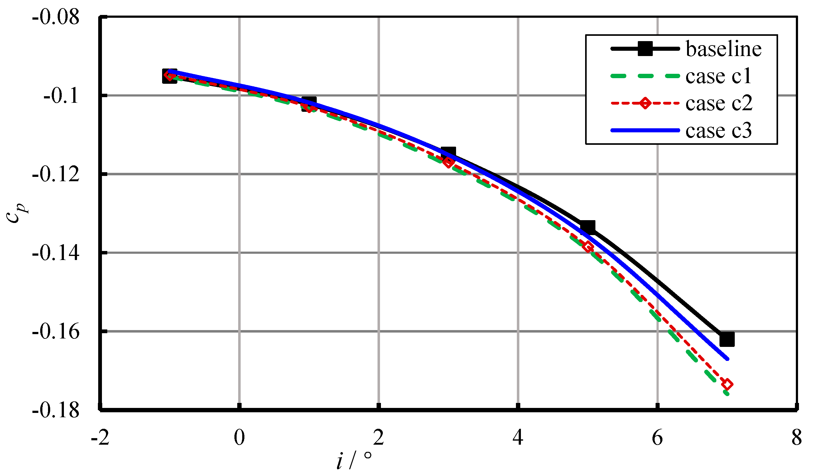
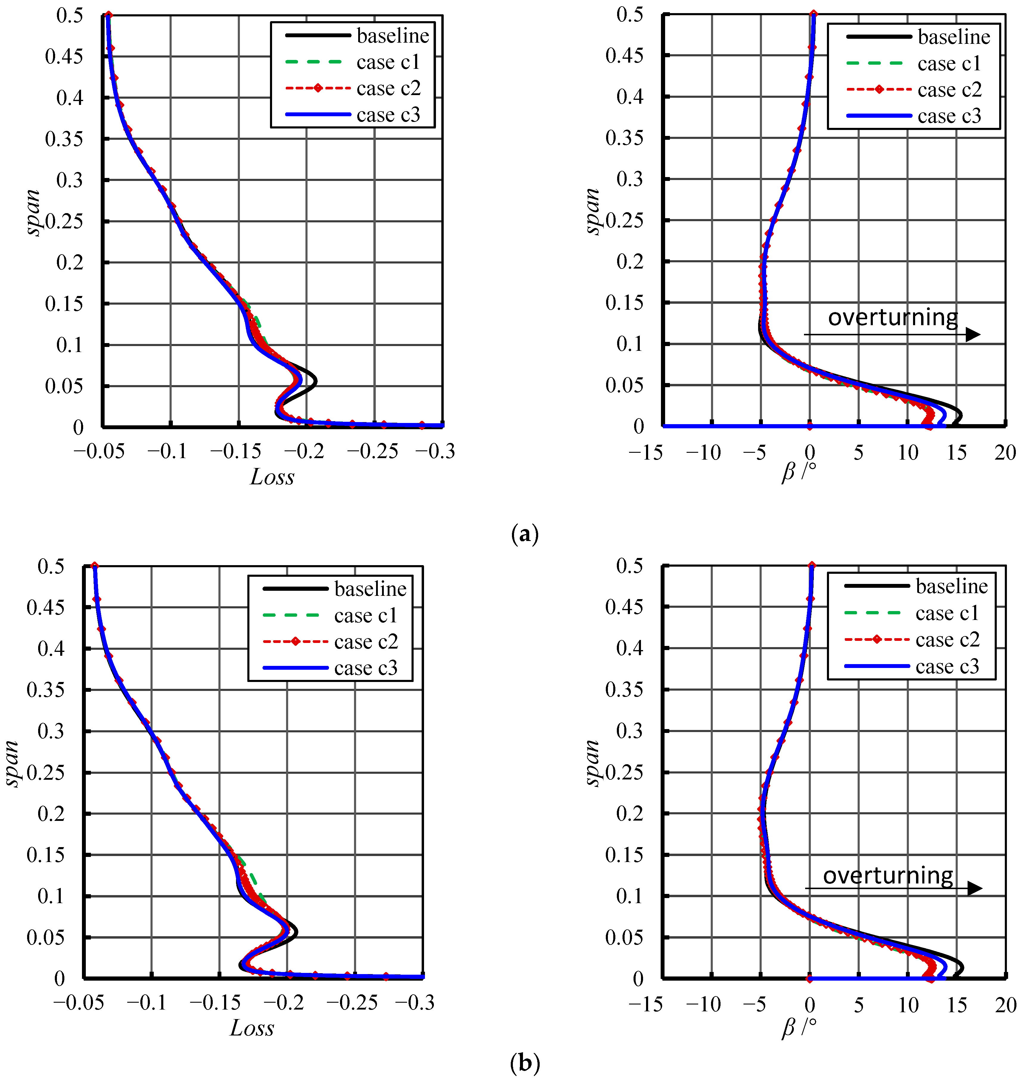
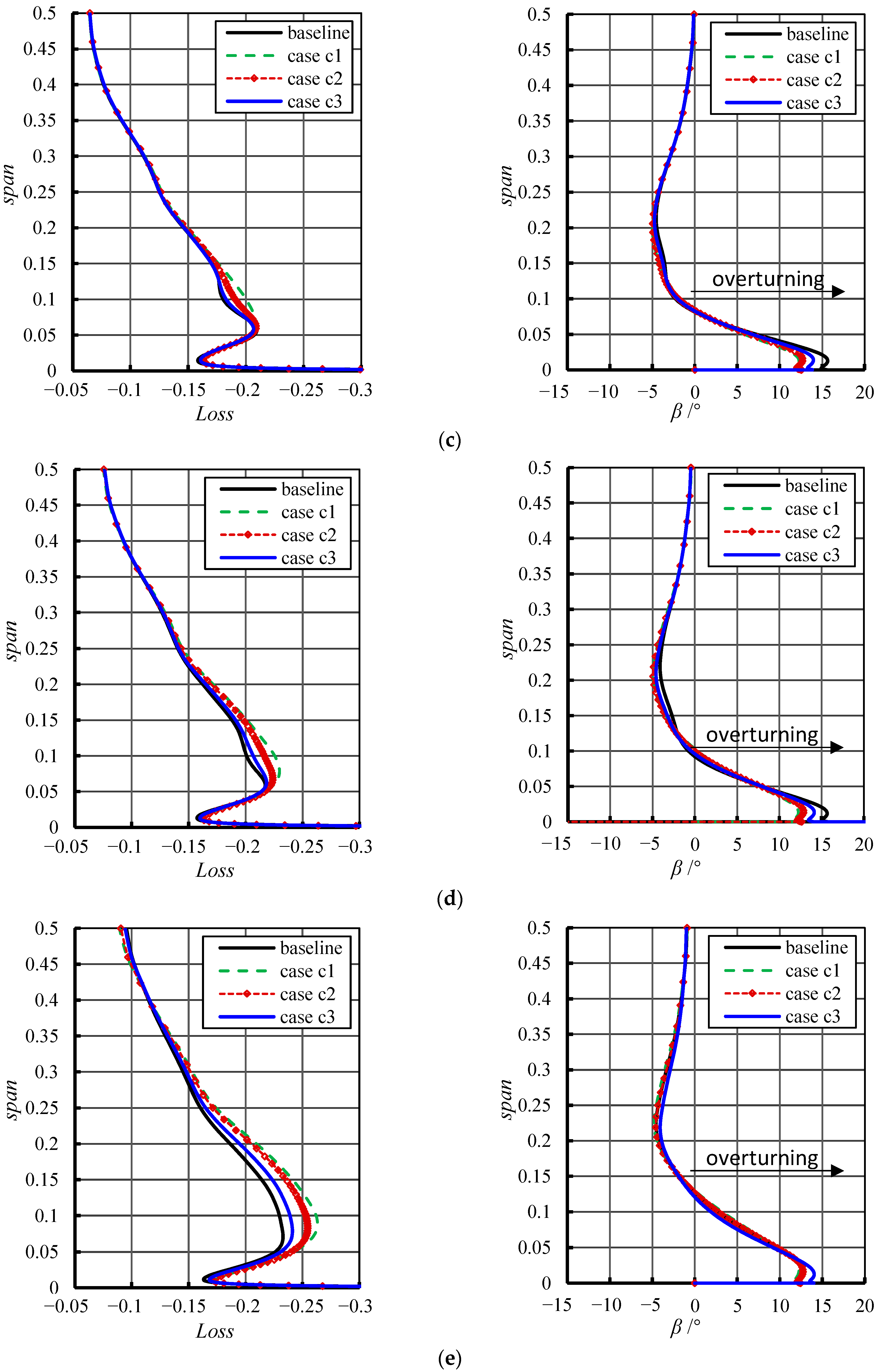
3.2. Results and Discussion

To apply the new method to the cascade, a software named PEWs was developed based on the newly proposed method and was used in this study. This software has a graphical interface for the design variables and enables up to 10 independent units for the end wall contouring. Three different groups of end wall contouring were designed using PEWs.

Table 3. The design parameter of the end wall contouring cases.

Cases	Parameters of the Full-Area Units		Parameters of the Localized Units
	Number	w	Number	ε1	ε2	ξ1	ξ2	w
c1	1	1	0	\	\	\	\	\
c2	1	0.5	1	0.4	0.9	0.9	0.1	0.5
c3	1	0.33	1	0.4	0.9	0.9	0.1	0.67

shows their main parameters. Figure 8 provides an overview of their geometry. The contours show the ratio between the end wall contouring height and the blade height ($\overline{H}$).

The first case simply uses a full-area unit. The geometry of end wall contouring forms an upslope from the SS to the PS. The aim is to reduce the transverse pressure gradient of the end wall region and decelerate the cross-passage secondary flow over the end wall range. This case is named c1. The geometry of case c1 is similar to the previously mentioned DPS in Ref. [7]. Thus, it represents the end wall contouring generated using a conventional empirical method.

The second and third cases both adopt a full-area unit and a localized unit to form the end wall contouring, named c2 and c3, respectively, to show their difference. Their design ideas come from previous research [4], which suggests that the end wall contouring should suppress the secondary flow over the end wall surface while accelerating the secondary flow near the SS corner. The difference between the two cases lies in the weight factors. The localized unit of case c3 has a greater weight than case c2, meaning that the latter tends to enhance the secondary flow locally in the SS corner more than the former.

Figure 9 gives the variation of the overall total pressure loss (c_p) with incidence (i) for the three end wall contouring cases. The working condition with i = −1° is the design point. Compared to case c1, case c2 and case c3 improve the performance of the cascade at the design point. Case c2 improves very little, and case c3 reduces the overall loss by about 0.13%; case c1, on the contrary, slightly increases the loss at the design point. As the incidence increases, the benefit of end wall contouring is gradually lost, but the ranking of the three cases is almost unchanged. When i exceeds +3°, all three end wall contouring cases, including case c3, result in a higher loss than the baseline cascade.

Corresponding to the overall performance, Figure 10 provides the spanwise distribution of total pressure loss and flow angle at 0.4C_a downstream of the TE. At the design point (Figure 10a), all three cases reduce Loss at 0.05span, indicating that the three cases have a comparable effect in suppressing the accumulation of low energy fluid at 0.05span. The difference is mainly between 0.08span and 0.15span, where case c1 and case c2 show larger Loss than the baseline case, and Loss in case c3 is roughly the same as the baseline case. The plots of β show stronger overturning for the baseline case than the end wall contouring cases, indicating that all three end wall contouring cases weaken the end wall secondary flow. Note the phenomenon here: case c3, which reduces the spanwise Loss most, does not correspondingly minimize the overturning, while case c1, which increases the spanwise Loss, shows the best control of the overturning in the end wall region.

As incidence gradually increases, the benefits of end wall contouring at 0.05span decrease, but the increment of Loss from the 0.08span to 0.15span of the end wall contouring cases becomes more significant than the baseline cascade. When the incidence is larger than 3°, the end wall contouring no longer significantly affects the distribution of Loss at 0.05span, and the phenomenon continues till the NS point (i = 7°); between 0.08span and 0.15span, the increase of Loss due to the end wall contouring grows significantly with the incidence. During the incidence increase, all end wall contouring cases show no significant increase of β.

The above results show that the influence of end wall contouring on the cascade mainly works in two areas:

Within 0.05span, the relief of the low-energy region due to the end wall contouring is the key to reducing the overall loss. The difference between cases c1, c2, and c3 is not significant, and this benefit gradually disappears with the increase of the incidence.

Between 0.08span and 0.15span, the different value of total pressure loss results in the difference among cases c1, c2, and c3. With the increase of the incidence, Loss of the end wall contouring cases gradually grows to be much higher than the baseline case, leading to a significant drop in their overall performance at large incidence.

In particular, Figure 11 shows the design point and the near stall point, giving the three-dimensional flow field of the baseline cascade and the end wall contouring cases near the end wall region.

At the design point (Figure 11a,c,e,g), the transparent grey area in the figures is the iso-surface of V_z = 0.1V_max, which indicates the development of separation in the corner region. The contours show the normalized turbulent viscosity (μ_t/μ) within the TE plane, representing the local shear loss caused by separation. The colored curves in the figure are the three-dimensional streamlines in the end wall region, and the color indicates its velocity magnitude. The iso-curve of the static pressure coefficient ($\overline{p}$) is plotted on the end wall and blade surface. $\overline{p}$ is defined as

$$\overline{p}=\frac{p-p_{\mathrm{in}}}{(p{t}_{\mathrm{in}}-p_{\mathrm{in}})}$$

(10)

Figure 11c shows that case c1 significantly weakens the cross-passage secondary flow. The significant changes are mainly reflected in three areas:

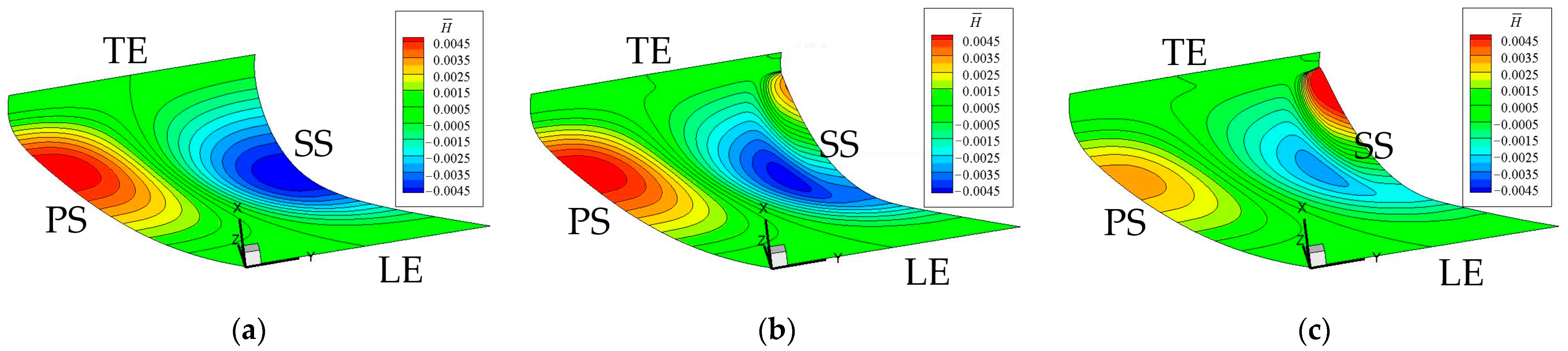
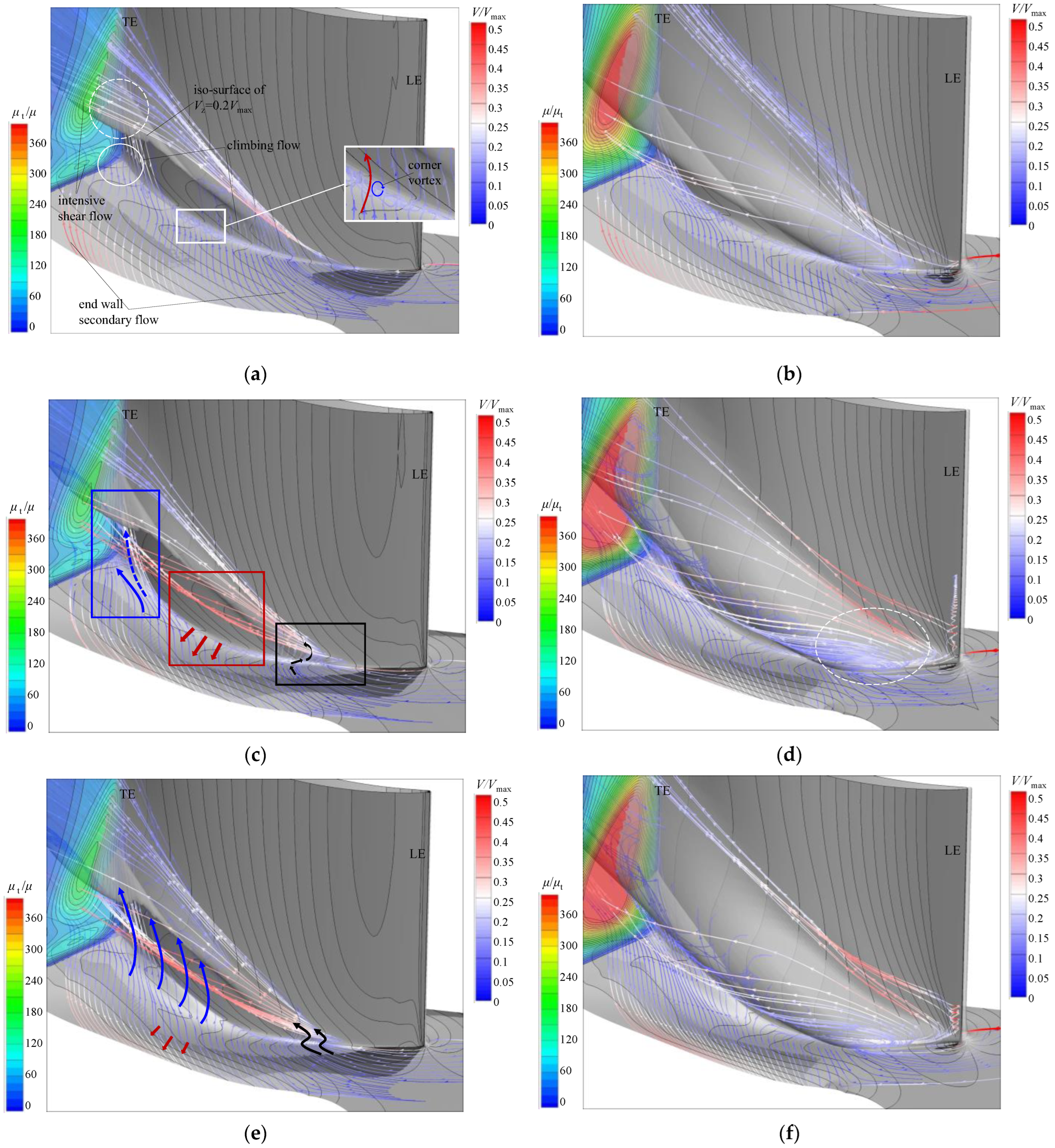
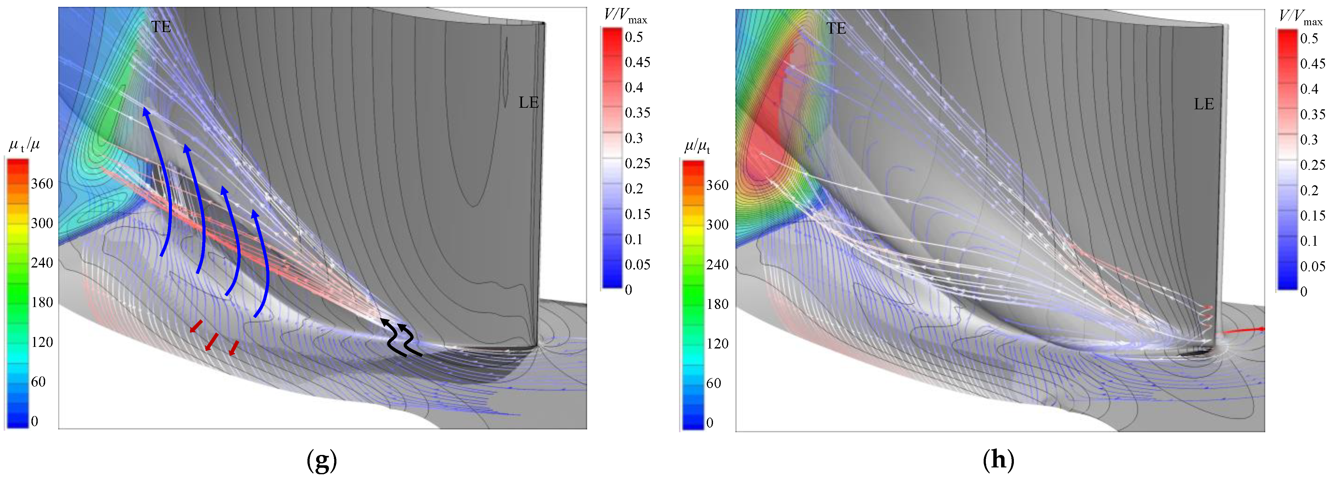
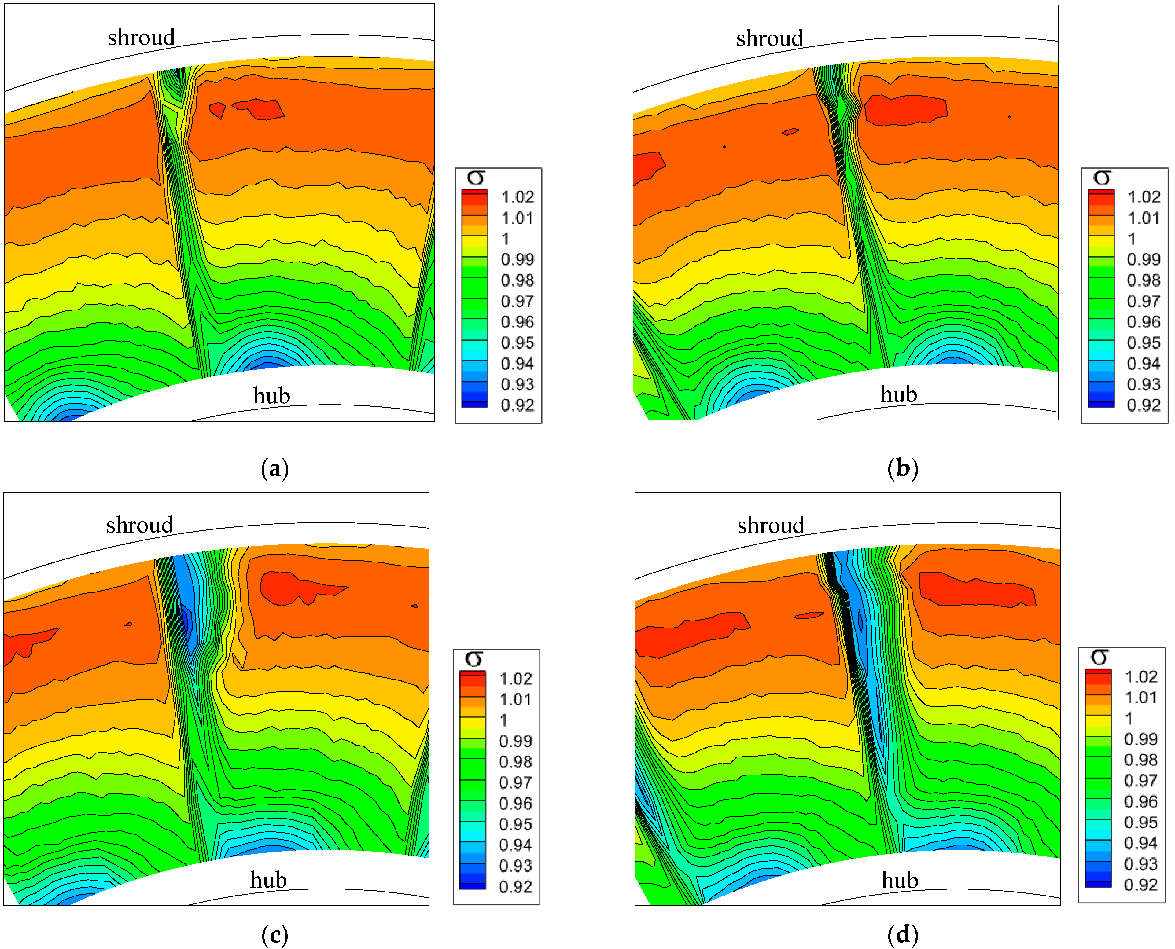
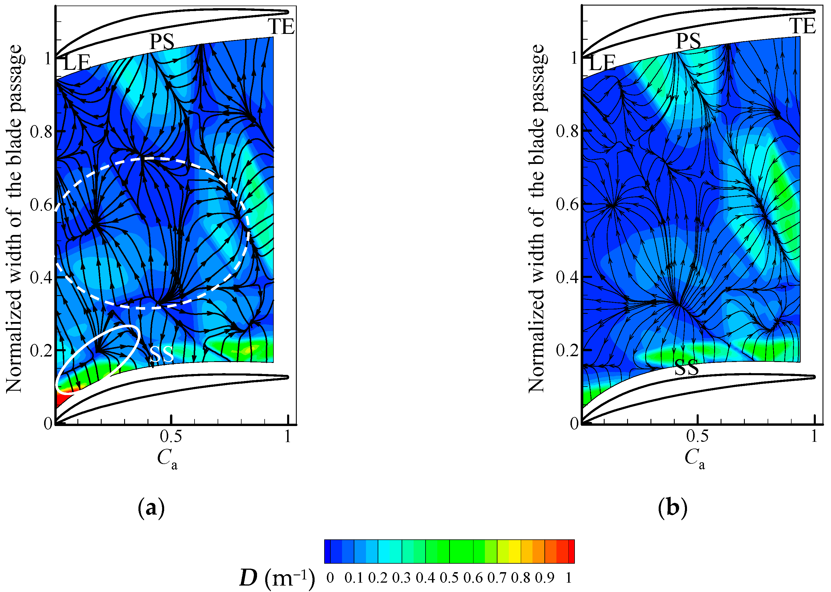
• First, the corner region near 0.2C_a to 0.4C_a from the LE (in the rightmost black box in Figure 11c), which, according to the streamlines, shows that this is precisely where the corner separation starts. The iso-curves of $\overline{p}$ show that the sinking end wall near the SS corner increases the pressure gradient significantly. Thus, the reverse flow is intensified, and more low-energy fluids accumulate in the corner region. This ultimately increases the local shear loss and exacerbates corner separation.
• Second, from the mid-chord to the rear region of the SS corner (located in the red box in the middle), the secondary climbing flow weakens, and the same is true for the cross trend of the end wall flow in the outer region (as shown by the red arrows). This is caused by the sinking surface of the end wall on the suction side. The weakened cross trend of end wall secondary flow will inhibit the accumulation of the low-energy fluid and thus help to reduce loss.
• Third, near the TE of the SS (in the blue box on the left), the end wall iso-curves of $\overline{p}$ show a high-density region, indicating that the streamwise pressure gradient is significantly reduced compared to the baseline case. This should be induced by the local streamwise upslope in the SS corner. This effect enhances the flow momentum of both the end wall flow (shown by the solid blue arrow) and its climbing motion after colliding with the SS (indicated by the dashed blue arrow). The acceleration of the climbing flow mixes with the low-energy fluid on the SS and increases its streamwise momentum. According to the contour of μ_t/μ at the TE plane, this “pre-mixing” effect reduces the shear effect between the separation flow and the main flow and thus brings benefits.

The correlation between the low-energy flow near the TE and upstream streamline is worth noting. According to the streamlines in the baseline cascade, the low-energy flow of the lower span at the TE plane (labeled with a solid white circle in Figure 11a) is associated with the secondary flow in the rear part of the corner region. In contrast, the low-energy flow of the higher span (labeled with a dashed white circle in Figure 11a) comes from the climbing flow along with the SS at the onset of separation in the upstream corner region. Because case c1 exacerbates the corner separation in the upstream SS corner, this indicates that the reduction of the Loss within 0.05span in Figure 10 comes from the second and third effects mentioned above, while the increase of Loss between 0.08span and 0.15span is mainly due to the first effect.

Compared to case c1, both case c2 and case c3 have less sinking end wall near the SS due to the localized unit. In the SS corner region from 0.2C_a to 0.4C_a, the iso-curves of $\overline{p}$ suggest that the inverse pressure gradient is lower than that of case c1, which makes the local inverse flow induced by case c2 and c3 less severe than that of case c1 (as shown by the black arrows in Figure 11e,g). As a result, the low-energy separation flow at the high span region near TE is also significantly reduced. Another region affected by the localized unit is the corner region from the 0.5C_a to the TE. The rise of the end wall near the corner region makes the climbing flow near the TE accelerate significantly and sweep downstream (as shown by the blue arrows in Figure 11e,g). This is consistent with the research in [4]. On the one hand, the energized secondary flow eliminates the low-energy flow in the corner vortex. More importantly, it enhances the “pre-mixing” effect of the secondary flow with the low-energy flow in the corner region mentioned in case c1. Therefore, it is more advantageous than case c1 here, and it can be seen from the TE plane’s μ_t/μ contour that the local shear loss is more minor than case c1. The weight factor of the localized unit in case c3 is larger than that of case c2, so the control of pressure gradient in the upstream SS corner and the enhancement of secondary flow pre-mixing near the trailing edge are more significant than that of case c2. The loss reduction in case c3 is, therefore, more significant.

The influence of end wall contouring at the near-stall point (i = 7°) is discussed similarly to the design point but more concisely. The flow field is shown in Figure 11b,d,f,h. Compared to the flow field in the design point, the differences between case c1 and the baseline case at the near-stall point are similar to those concluded at the design point. It also appears that the pressure gradient in the SS corner area from 0.2C_a to 0.4C_a increases significantly, the secondary climbing flow from the SS corner between 0.5C_a and TE weakens, and the streamwise pressure gradient near the TE of SS reduces. However, the main difference is that the corner separation at the LE of the cascade is much more severe than the design point (labeled using a dashed white circle in Figure 11d). The local pressure gradient increase due to the sinking end wall intensifies the reverse flow trend, making the corner separation stronger after its generation. This effect amplifies the negative impact of the end wall contouring on the flow field of the cascade between 0.2C_a and 0.4C_a, finally leading to an overall loss increase. Thus the contour of μ_t/μ shows that the low-energy separation flow causes much higher shear losses than the baseline cascade when it develops to the TE.

The advantages of cases c3 and c2 over case c1 are still significant. Under the influence of the localized unit, case c3 and case c2 show more mitigated upstream corner reverse flow and more intense downstream pre-mixing effect of the separation flow than case c1. Therefore, the control of separation loss in cases c2 and c3 is better than case c1. case c3 leads to the slightest increase in loss among all end wall contouring cases due to its larger weight factor of the localized unit than case c2.

In summary, although the corner separation is still not effectively suppressed at the near-stall point, the new end wall contouring method shows its potential for flow control, especially when combined with the previous experience. As already mentioned at the beginning of Section 3, case c1 represents the DPS designed by the traditional empirical method. In comparison, the cases using two end wall contouring units perform better under more than one incidence. What’s more, the intended flow control of the full-area and localized units, including the effect of their weight factors, agrees very well with their effects during the application. All these indicate that the new end wall contouring method is superior to the traditional empirical method.

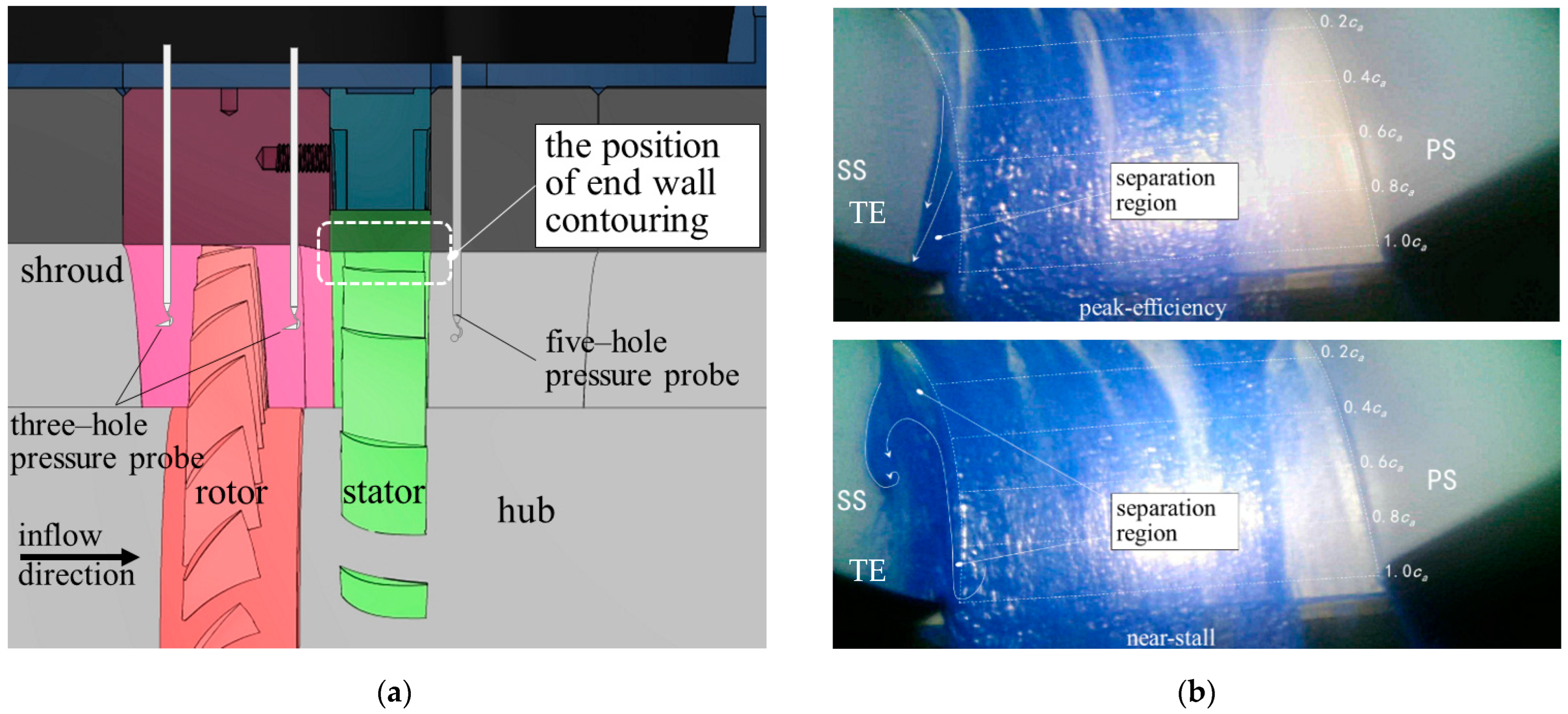
4. Experiment on the Axial Compressor Test Rig

The following will check the performance of the new end wall contouring method in an axial compressor through an experiment.

4.1. The Baseline Compressor Stage and the Design of End Wall Contouring

The compressor of the test rig is a single-stage high-speed axial flow compressor from Northwestern Polytechnic University, as sketched in Figure 12a. The testing stations for the total pressure of the compressor flow field are also illustrated. The diameter of the rotor is 298 mm, with a design speed of 15,200 rpm. Experimental and numerical research on this stage confirmed that when the rotor speeds up to 70% of the design speed, the rotation will reach a relatively steady state for the stator testing, and there will be a considerable corner separation in the casing end wall region of its stator, as shown in the oil-flow photos in Figure 12b. The experiment thus designs end wall contouring on the casing of the stator to improve the performance of the compressor operating at 70% speed.

According to the numerical results in the cascade, constructing a concave surface in the front SS corner would raise the pressure gradient and negatively affect the initiation of corner separation, especially when the incidence increases. Therefore, the new design shows an improvement and adopts three units, with the parameters shown in

Table 4. The design parameter of the end wall contouring for the stator.

Parameters of the Full-Area Units		Parameters of the Localized Units
Number	w	Number	ε1	ε2	ξ1	ξ2	w
0	0	3	0.2; 0.5; 0.1	0.7; 0.8; 0.3	0.5; 0.85; 0.7	1; 1; 1	−0.25; 0.5; 0.25

. The first unit is to suppress the end wall second flow. Here, we use a localized unit with a large profiling area instead of a full-area unit to prevent aggravating the reverse flow in the front SS corner. Its design parameter is listed in the first place of each blank, i.e., ε₁ = 0.2, ε₂ = 0.7, ξ₁ = 0.5, ξ₂ = 1, and w₁ = −0.25. The second localized unit aims to accelerate the secondary climbing flow in the rear part of the SS corner, so the pitch-wise range of the second localized unit is limited to 15% of the circumferential width of the passage (defined with w) beyond the SS in the rear half of the SS. The third localized unit aims to reduce the potential negative effect in the front SS corner area. The range of this unit thus spreads within 30% w from the SS, forming a mild upslope surface to reduce the sinking end wall due to the first localized unit. Figure 13 shows the geometry of the end wall contouring and the photo of the experimental part.

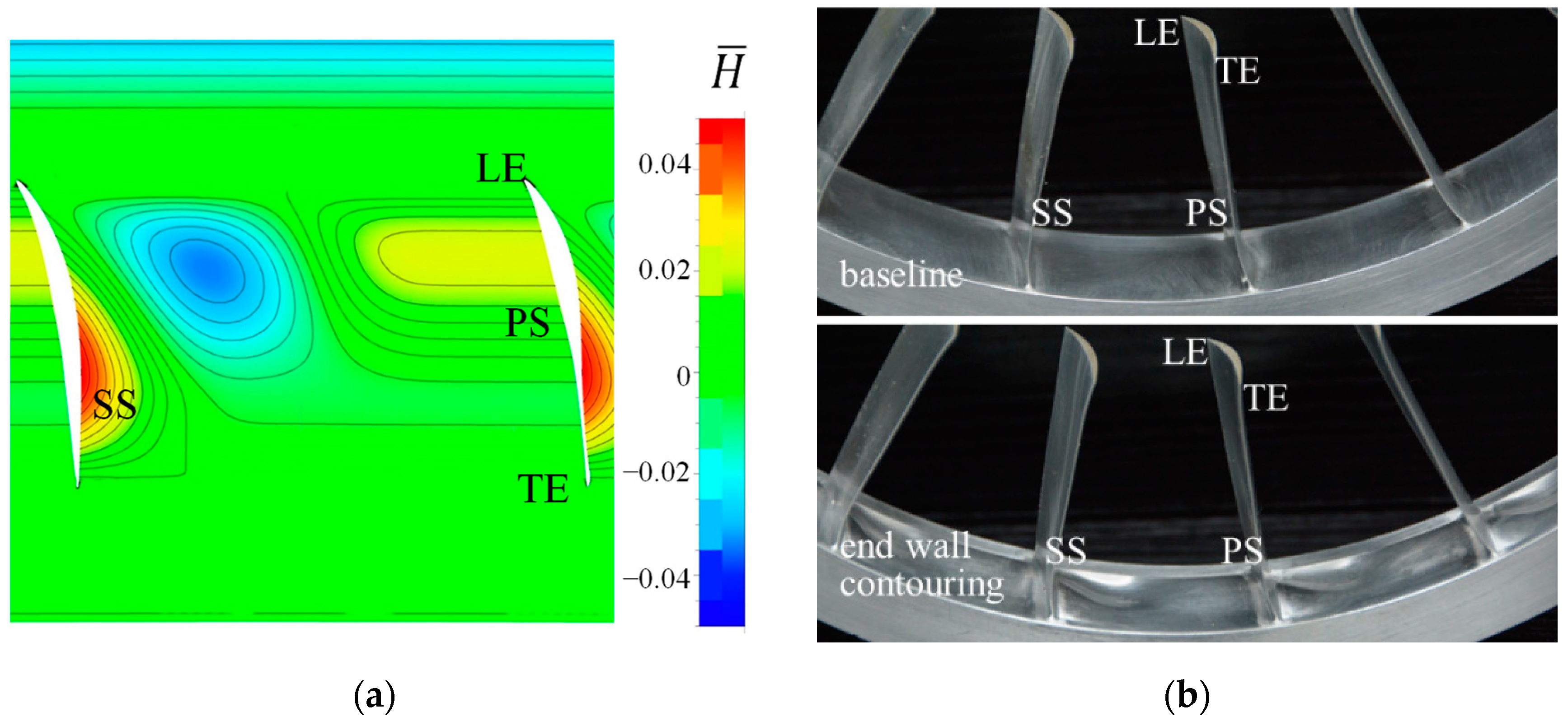
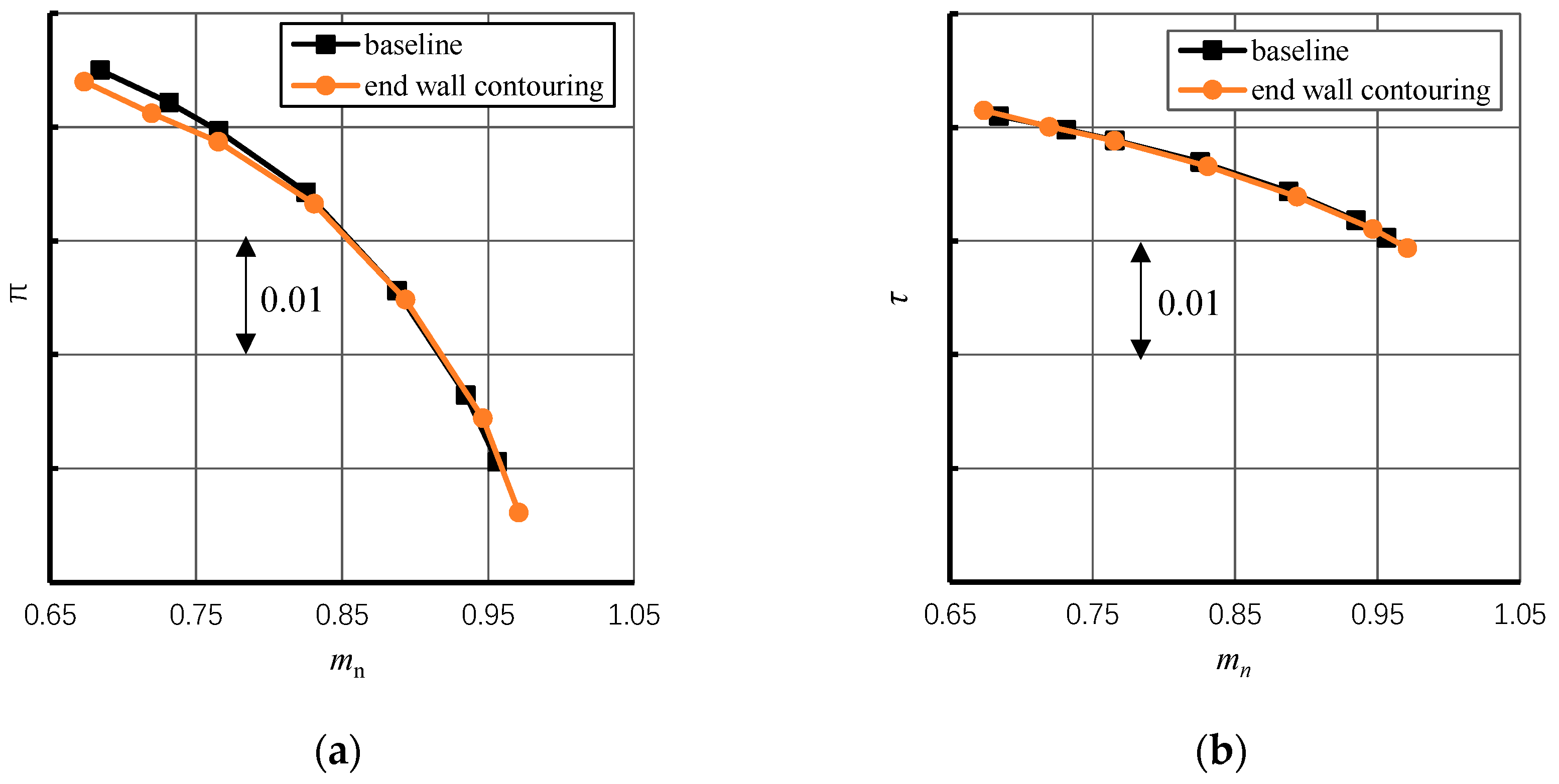
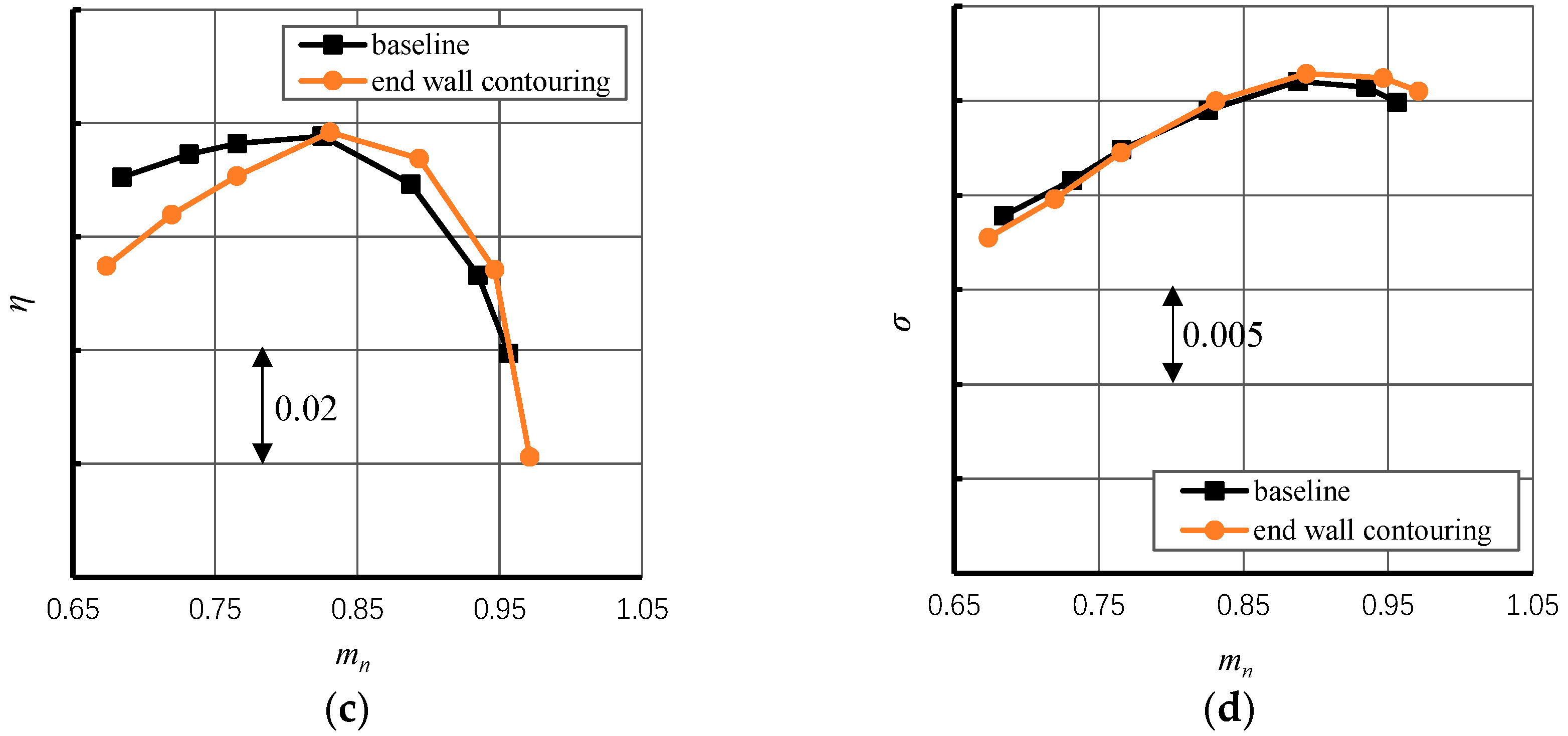
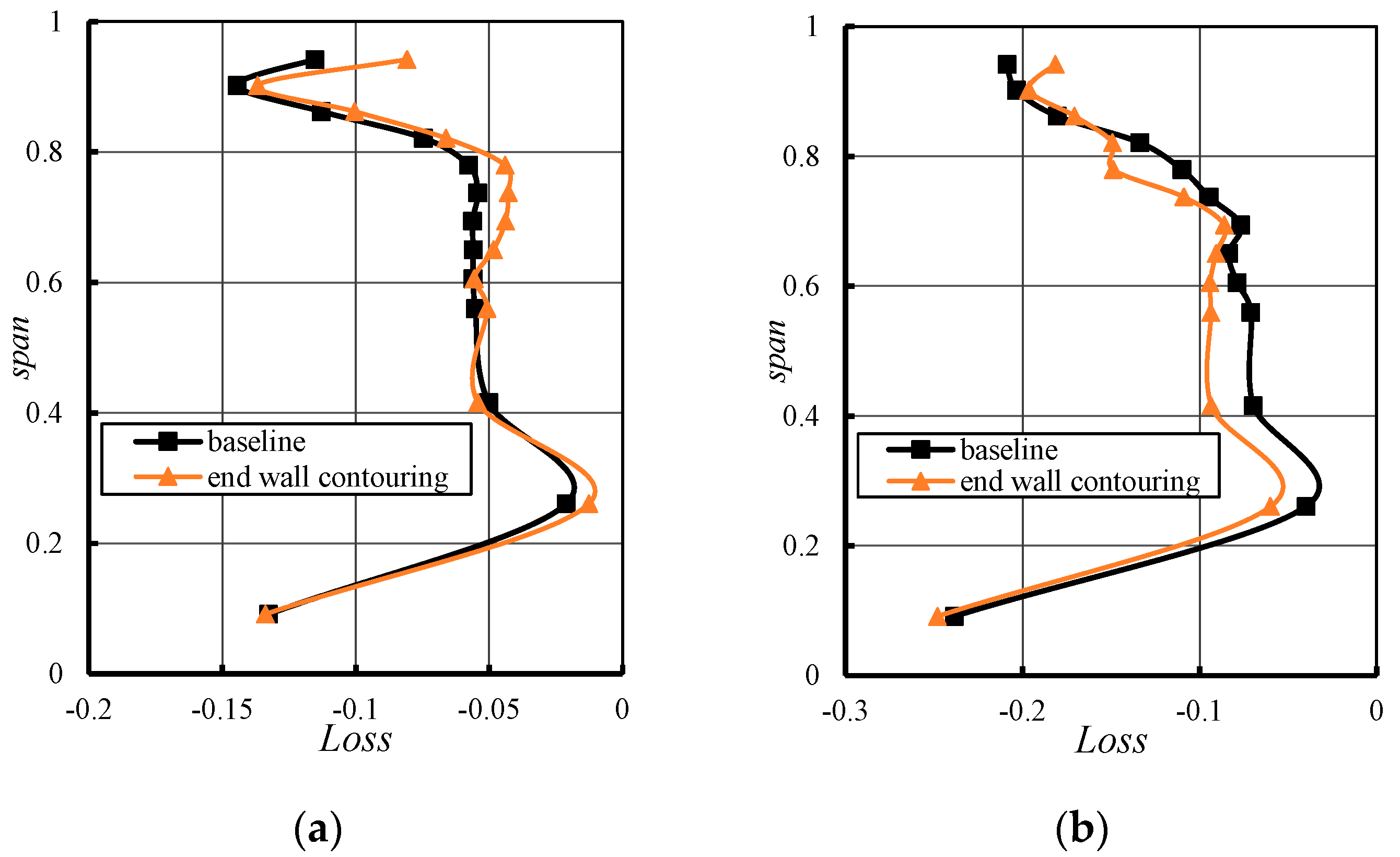
4.2. Results and Discussion

Figure 14 compares the overall performance of the stage before and after end wall profiling. The experimental results confirmed the positive effect of end wall contouring on the flow field when $\overline{m}$ > 0.83. The full-stage efficiency improved by 0.45% at the working point of minimum stator loss (the normalized mass flow rate $\overline{m}$ equals 0.89). Note that the total temperature ratio in Figure 14b is generally the same before and after the end wall contouring, while the variation of the total pressure recovery coefficient (σ) of the stator in Figure 14d is very similar to the efficiency. The variation of σ shows that the total pressure loss in the stator is reduced by 10.44% of its original value. Thus, the change of efficiency should be mainly associated with the stator loss rather than the rotor work. The stall margin does not change much. It is noted that end-wall shaping does not improve the total pressure ratio and efficiency when $\overline{m}$ < 0.83. Thus, the specific effect of end wall contouring on the stator casing flow field will be discussed in the next step.

Figure 15 selects two specific working points and compares the stators’ circumferential averaged total pressure loss before and after end wall contouring. One is the working point with the minimum stator loss ($\overline{m}$ = 0.89). Herein, it is termed the best-matching point for brevity, abbreviated as “BM.” Another is a working point during the throttling process ($\overline{m}$ = 0.77), closer to the near-stall point but still relatively stable for the experiment. It is termed the left-map working point in the following passage, abbreviated as “LM.” At the LM point, the variation of σ indicates the overall total pressure loss increases by 1.95% of its original value.

At the BM point, the end wall contouring shows a noticeable effect on reducing end wall loss. According to the experimental data in Figure 15a, the total pressure loss coefficient decreases by about 0.01 from 0.7span to the blade tip and nearly remains the same in other regions. The reduction of the total pressure loss reaches 0.035 above 0.9span and 0.01–0.013 from 0.8span to 0.9span. The two-dimensional distribution of σ in the outlet plane of the stator is given in Figure 16a,b. This reveals that the low value of σ significantly reduces and moves farther away from the end wall than the baseline stator. This is apparently consistent with the mechanism in the cascade and previous research [4,9].

At the LM point, the effect of end wall contouring on the loss coefficient extends significantly from the blade top to the full-span region. Figure 15b shows that the loss coefficient reduces by 0.01–0.03 above 0.85span, increases by 0.01–0.03 from 0.7span to 0.85span, and increases up to 0.023 from 0.6span to the hub. The variation of loss coefficiency from 0.7span to the blade tip region should be affected by the end wall contouring. Although part of this region increases the loss coefficient, this still shows more benefit than case c3 in the cascade: the loss coefficient close to the end wall reduces (Figure 15b), and the core region of low σ at 0.75span is slightly relieved (Figure 16d). However, the range from 0.6span to the hub is beyond the end wall contouring’s direct influence. In Figure 16d, the corresponding region shows a heavier wake in the end wall contouring case, indicating a greater blade profile loss than the baseline stator. Thus, the increase of loss below 0.6span should be associated with the spanwise variation of the throughflow under the same mass flow rate. It should be the end wall contouring that relieves the blockage due to corner separation on the top side of the blade passage, thereby reducing the mass flow rate of the lower span range. As a result, the lower part of the passage is more throttled than ever, thus generating a higher loss in return.

The above study generally verifies the effect of end wall contouring on the control of corner separation and its contribution to the compressor’s performance. However, it is still uncertain whether the control of secondary flow that leads to these improvements is consistent with the design intent shown by the variables in Table 4. This is further verified below with the testing result from the end wall pressure taps.

It is known that near the end wall region, the boundary layer motion should obey the N-S equation, i.e.,

$$\frac{\partial \mathit{V}}{\partial t}+\mathit{V}\nabla \mathit{V}=-\frac{1}{\rho }\nabla p+\tau$$

(11)

Suppose the end wall contouring surface has a relatively slight waviness to the scale of the chord length, and the flow is constant; in this case, the N-S equation on the end wall surface before and after the end wall contouring can be subtracted to obtain

$${\mathit{V}}_{\mathrm{EWC}}\nabla {\mathit{V}}_{\mathrm{EWC}}-{\mathit{V}}_{\mathrm{baseline}}\nabla {\mathit{V}}_{\mathrm{baseline}}=-\frac{1}{\rho }\nabla (P_{\mathrm{EWC}}-P_{\mathrm{baseline}})+{\mathit{\tau }}_{\mathrm{EWC}}-{\mathit{\tau }}_{\mathrm{baseline}}$$

(12)

where the subscripts “EWC” and “baseline” represent the aerodynamic parameters before and after using the end wall contouring, and their subtraction result thus represents the variation of the parameters at the corresponding position on the S1 flow surface. The left side is the variation of the acceleration due to the end wall contouring, which directly changes the secondary flow on the end wall surface. Thus, the variation of pressure gradient on the right side of Equation (12) should be the primary cause for the left-side items, and thus the end wall secondary flow and corner separation. Taking into account the convenience of the testing, here we define a new variable from the static pressure taken by the end wall pressure taps according to

$$\mathit{D}=-(\nabla {(\frac{p}{p_{t0}})}_{\mathrm{EWC}}-\nabla {(\frac{p}{p_{t0}})}_{\mathrm{baseline}})$$

(13)

where p_t0 represents the inlet total pressure of the rotor. The variable D represents a quantitative measure of the driving force of the end wall contouring on the end wall secondary flow. The magnitude of D is plotted in Figure 17, and the arrow illustrates its direction.

The contour of the BM point shows clear correspondence with the previously mentioned design intent. From LE to the 0.3C_a, a high value of D pointing to the SS (marked with a white dashed circle) agrees with the intent of the third localized unit. A wide range of D pointing to the PS (marked with a solid white circle) spreads from the outer SS corner to the middle of the channel. This is associated with the second localized unit. Downstream of 0.4C_a, the direction of D near the SS corner points to SS from 0.4C_a to 0.7C_a and then points to the PS direction downstream of 0.7C_a. The distribution of D here is partially associated with the flow control intent of the first localized unit, except for the region after 0.7C_a. This is likely related to the downslope surface at the end wall, i.e., the side effect of the localized unit mentioned in Section 2.

Compared to the BM point, the magnitude of D spreading along the SS corner area generally decreases at the LM point. The changes of D with the working condition are not significant. The primary difference lies in the front SS corner, where the direction of D changes to the PS direction. It is possibly related to the reverse flow caused by the separation at the LE corner region, but it can be seen from the figure that the D is not opposed to the streamwise direction. Thus, this shows that end wall contouring somewhat avoids the aggravation of reverse flow caused by the first localized unit. It may likely explain why the end wall contouring, in this case, improves the flow field in the end wall area even at the LM working point.

4.3. Summary of the Effects of the End Wall Contouring

According to the overall performance, the end wall contouring only benefits the right-side operating map of the compressor stage. At the BM point of the compressor, the end wall contouring increases the peak value of σ in the stator, thus making a 10.44% relative reduction of stator loss, which finally increases the overall efficiency by 0.45%. At the LM point, the decrease of σ shows the stator loss increases relatively by 1.95%. Thus, the overall efficiency of the stage decreases by 1.5%.

However, although the efficiency does not increase in all the working conditions, the flow field shows that applying the new end wall contouring method can always improve the corner separation. The tested end wall static pressure shows that the end wall contouring suppresses the end wall secondary flow in the full range but accelerates the cross and climbing flow in the SS corner. The corner separation is thus reduced, and the total pressure loss coefficient in the end wall region reduces locally by 0.01–0.03 for both the operating points.

For the reduction of efficiency at the LM point, the experimental data show it is likely a side effect of suppressing the corner separation. Because the relief of corner separation reduces the local blockage, the throughflow increases in the end wall region and decreases in the main flow. As a result, the main flow region is more “throttled”, thus negatively affecting the control of loss. It should be noted that this side effect does not have to increase loss. Just as reported in Hu’s research [7], if the main flow is robust, suppressing the corner separation will not increase the loss in the main flow region. Otherwise, it could induce a detrimental effect, as in Reising’s research [18], where severe corner separation occurs in the opposite end wall and threatens the stall margin. Considering that even applying an end wall suction of the boundary layer has been reported to increase the loss of main flow [28], the side effect mentioned above should be regarded as a common limitation for all the end wall flow control techniques. The blade row’s sensitivity to throttling determines whether or not the loss will increase and how much it will increase. So, for the LM point of the current study, the efficiency reduction reflects that the effect of the end wall contouring was limited by the characteristics of the current compressor stator. The problem may be solved by improving the blade profile.

Above all, the numerical and experimental results indicate that when applying the newly developed end wall contouring method, the intended control of secondary flow in the design space agrees with its actual effect and effectively suppresses the corner separation under multiple inflow conditions. Thus, the results prove its effectiveness. If looking at the empirical end wall contouring method in previously reported studies, the traditional empirical method typically constructs the full area of the end wall surface uniformly through a single analytical formula [2,7,8] or by manual adjustment [9]. In comparison, the newly developed method enables the parametric end wall to control secondary flow in more than one local region under multi-operating conditions. Thus, the control of secondary flow will be more adaptable to different compressors and produce a much closer result to the optimization design, with a relatively small number of design variables. Moreover, in the current new empirical method, the design variables show not only an intuitive effect on the geometry but also a clear relation with the movement of the secondary flow. The new method is thus more convenient for concluding the design experience and shows a possibility to be applied in an optimization process.

5. Conclusions

This study proposes a new end wall contouring method based on the secondary flow control mechanism established in previous research, then verified its effectiveness numerically in a cascade and experimentally in an axial compressor stage. The following conclusions were obtained:

• The idea of the new end wall contouring method is to define multiple standard surface “units” with particular effects on the end wall secondary flow. Then, we apply a weighted superposition to the units to obtain a comprehensive flow control effect. Compared with the traditional empirical method in the previous research, the design space of the new method enables the parametric end wall to control secondary flow intuitively in more than one local region with a proper amount of design variables, thus showing more advantages.
• The numerical and experimental research indicates two primary mechanisms of applying the end wall contouring to control the corner separation, i.e., the local acceleration of secondary flow at the SS corner and the full-range deceleration of the secondary flow in the rear passage. The former will accelerate the corresponding secondary climbing flow on the SS, thus mixing with the low-energy separation flow and reducing the separation loss. The latter will suppress the accumulation of low-energy fluid of the boundary layer at the SS corner, thus relieving the local reverse flow. However, the above flow control may also be accompanied by the negative effect of the inverse pressure gradient at the front SS corner, which may seriously deteriorate the corner separation when it is under high incidence.
• When applied to the stator casing end wall of an axial compressor, although the efficiency only increases on the right part of the operating map, the experiment results show that the intended control of secondary flow agrees with its actual effect and suppresses the corner separation under multiple operating conditions. Its effectiveness is thus verified. The reduction of efficiency at the small mass-flow-rate working points reflects a limitation of the new method and is probably associated with the characteristics of the current compressor stator.

The number of design variables in the newly developed end wall contouring method is relatively small, and all of them show a clear and intuitive effect on the secondary flow. The next step of the research should consider the optimization process. Three-dimensional blading should also be included to overcome any shortages when suppressing the corner separation.

References

- Rose, M.G. Non-Axisymmetric Endwall Profiling in the HP NGV’s of an Axial Flow Gas Turbine. In Proceedings of the ASME Turbo Expo, The Hague, The Netherlands, 13–16 June 1994. 94-GT-249. [Google Scholar]
- Meng, T.; Yang, G.; Zhou, L.; Ji, L. Full blended blade and endwall design of a compressor cascade. Chin. J. Aeronaut. 2021, 34, 79–93. [Google Scholar] [CrossRef]
- Ma, Y.; Teng, J.; Zhu, M.; Qiang, X. Non-axisymmetric Endwall Contouring in a Linear Compressor Cascade. In Proceedings of the ASME Turbo Expo 2020, London, UK, 21–25 September 2020. GT2020-14366. [Google Scholar]
- Li, X.; Chu, W.; Wu, Y.; Zhang, H.; Spence, S. Effective end wall profiling rules for a highly loaded compressor cascade. Proc. Inst. Mech. Eng. A J. Power Energy 2016, 230, 535–553. [Google Scholar] [CrossRef] [Green Version]
- Liu, X.; Jin, D.; Gui, X.; Liu, X.; Guo, H. Effect of Solidity on Non-Axisymmetric Endwall Contouring Performance in Compressor Linear Cascades. In Proceedings of the ASME Turbo Expo, Oslo, Norway, 11–15 June 2018. GT2018-76247. [Google Scholar]
- Ma, Y.; Teng, J.; Zhu, M.; Qiang, X. Influence of the inlet boundary layer on non-axisymmetric endwall contouring effects in a linear compressor cascade. Proc. Inst. Mech. Eng. C J. Mech. Eng. Sci. 2022. [Google Scholar] [CrossRef]
- Hu, S.; Lu, X.; Zhang, H.; Zhu, J.; Xu, Q. Numerical Investigation of a High-subsonic Axial-flow Compressor Rotor with Non-axisymmetric Hub Endwall. J. Therm. Sci. 2010, 19, 14–20. [Google Scholar] [CrossRef]
- Cao, Z.; Gao, X.; Liu, B. Control mechanisms of endwall profiling and its comparison with bowed blading on flow field and performance of a highly-loaded compressor cascade. Aerosp. Sci. Technol. 2019, 95, 105472. [Google Scholar] [CrossRef]
- Harvey, N.W. Some Effects of Non-Axisymmetric End wall Profiling on Axial Flow Compressor Aerodynamics. Part I: Linear Cascade Investigation. In Proceedings of the ASME Turbo Expo, Berlin, Germany, 9–13 June 2008. GT2008-50990. [Google Scholar]
- Reising, S.; Schiffer, H. Non-axisymmetric end wall profiling in transonic compressors. Part II: Design study of a transonic compressor rotor using nonaxisymmetric end walls optimization strategies and performance. In Proceedings of the ASME Turbo Expo, Orlando, FL, USA, 8–12 June 2009. GT2009-59134. [Google Scholar]
- Zhang, X.; Lu, X.; Zhu, J. Performance Improvements of a Subsonic Axial-Flow Compressor by Means of a Non-Axisymmetric Stator Hub End-Wall. J. Therm. Sci. 2013, 22, 539–546. [Google Scholar] [CrossRef]
- Dorfner, C.; Hergt, A.; Nicke, E.; Moenig, R. Advanced Nonaxisymmetric End wall Contouring for Axial Compressors by Generating an Aerodynamic Separator- Part I: Principal Cascade Design and Compressor Application. J. Turbomach. 2011, 133, 021026. [Google Scholar] [CrossRef]
- Hergt, A.; Dorfner, C.; Steinert, W.; Nicke, E.; Schreiber, H. Advanced Nonaxisymmetric End wall Contouring for Axial Compressors by Generating an Aerodynamic Separator- Part II: Experimental and Numerical Cascade Investigation. J. Turbomach. 2011, 133, 021027. [Google Scholar] [CrossRef]
- Reutter, O.; Hemmert-Pottmann, S.; Hergt, A.; Nicke, E. Endwall contouring and fillet design for reducing losses and homogenizing the outflow of a compressor cascade. In Proceedings of the ASME Turbo Expo, Düsseldorf, Germany, 16–20 June 2017. GT2014-25277. [Google Scholar]
- Huang, S.; Yang, C.; Li, Z.; Han, G.; Zhao, S.; Lu, X. Effect of Non-Axisymmetric End Wall on a Highly Loaded Compressor Cascade in Multi-Conditions. J. Therm. Sci. 2021, 30, 1363–1375. [Google Scholar] [CrossRef]
- Harvey, N.W.; Offord, T.P. Some Effects of Non-Axisymmetric End wall Profiling on Axial Flow Compressor Aerodynamics. Part II: Multi-Stage HPC CFD Study. In Proceedings of the ASME Turbo Expo, Berlin, Germany, 9–13 June 2008. GT2008-50991. [Google Scholar]
- Varpe, M.K.; Pradeep, A.M. Benefits of nonaxisymmetric endwall contouring in a compressor cascade with a tip clearance. J. Fluids Eng. 2015, 137, 051101. [Google Scholar] [CrossRef]
- Reising, S.; Schiffer, H. Non-axisymmetric end wall profiling in transonic compressors. Part I: Improving the static pressure recovery at off-design conditions by sequential hub and shroud end wall profiling. In Proceedings of the ASME Turbo Expo, Orlando, FL, USA, 8–12 June 2009. GT2009-59133. [Google Scholar]
- Lepot, I.; Mengistu, T.; Hiernaux, S. Highly Loaded LPC Blade and Non Axisymmetric Hub Profiling Optimization for Enhanced Efficiency and Stability. In Proceedings of the ASME Turbo Expo, Vancouver, BC, Canada, 6–10 June 2011. GT2011-46261. [Google Scholar]
- Li, X.; Chu, W.; Wu, Y. Numerical investigation of inlet boundary layer skew in axial-flow compressor cascade and the corresponding non-axisymmetric end wall profiling. Proc. Inst. Mech. Eng. A J. Power Energy 2014, 228, 638–656. [Google Scholar] [CrossRef]
- Ji, L.; Tian, Y.; Li, W.; Yi, W.; Wen, Q. Numerical Studies on Improving Performance of Rotor-67 by Blended Blade and Endwall Technique. In Proceedings of the ASME Turbo Expo, Copenhagen, Denmark, 11–15 June 2012. GT2012-68535. [Google Scholar]
- Mahmood, S.; Turner, M.; Siddappaji, K. Flow Characteristics of an Optimized Axial Compressor Rotor Using Smooth Design Parameters. In Proceedings of the ASME Turbo Expo, Seoul, Korea, 13–17 June 2016. GT2016-57028. [Google Scholar]
- Cheng, J.; Chen, J.; Xiang, H. A Surface Parametric Control and Global Optimization Method for Axial Flow Compressor Blades. Chin. J. Aeronaut. 2019, 32, 1618–1634. [Google Scholar] [CrossRef]
- Sun, S.; Chen, S.; Liu, W.; Gong, Y.; Wang, S. Effect of Axisymmetric Endwall Contouring on the High-load Low-reaction Transonic Compressor Rotor with a Substantial Meridian Contraction. Aerosp. Sci. Technol. 2018, 81, 78–87. [Google Scholar] [CrossRef]
- Brennan, G.; Harvey, N.W.; Rose, M.G.; Fomison, N.; Taylor, M.D. Improving the Efficiency of the Trent 500-HP Turbine Using Nonaxisymmetric End Walls—Part I: Turbine Design. ASME J. Turbomach. 2003, 125, 497–504. [Google Scholar] [CrossRef]
- Zhang, Y.; Mahallati, A.; Benner, M. Experimental and numerical investigation of corner stall in a highly-loaded compres-sor cascade. In Proceedings of the ASME Turbo Expo, Düsseldorf, Germany, 16–20 June 2014. GT2014-27204. [Google Scholar]
- Akcayoz, E.; Vo, H.D.; Mahallati, A. Controlling Corner Stall Separation with Plasma Actuators in a Compressor Cascade. In Proceedings of the ASME Turbo Expo, Montreal, QC, Canada, 15–19 June 2015. GT2015-43404. [Google Scholar]
- Lu, H.; Wang, X.; Guo, S.; Huang, Y.; Zheng, Y.; Zhang, H.; Zhong, J. The Numerical Investigation of Asymmetric Boundary Layer Suction in High-load Compressor Cascades. J. Eng. Thermophys. 2018, 39, 977–984. [Google Scholar]