Article

Large-Scale Truss Topology and Sizing Optimization by an Improved Genetic Algorithm with Multipoint Approximation

School of Astronautics, Beihang University, Beijing 100191, China
*
Author to whom correspondence should be addressed.
Appl. Sci. 2022, 12(1), 407; https://doi.org/10.3390/app12010407
Submission received: 24 November 2021 / Revised: 16 December 2021 / Accepted: 23 December 2021 / Published: 31 December 2021

Abstract

:
Truss size and topology optimization problems have recently been solved mainly by many different metaheuristic methods, and these methods usually require a large number of structural analyses due to their mechanism of population evolution. A branched multipoint approximation technique has been introduced to decrease the number of structural analyses by establishing approximate functions instead of the structural analyses in Genetic Algorithm (GA) when GA addresses continuous size variables and discrete topology variables. For large-scale trusses with a large number of design variables, an enormous change in topology variables in the GA causes a loss of approximation accuracy and then makes optimization convergence difficult. In this paper, a technique named the label–clip–splice method is proposed to improve the above hybrid method in regard to the above problem. It reduces the current search domain of GA gradually by clipping and splicing the labeled variables from chromosomes and optimizes the mixed-variables model efficiently with an approximation technique for large-scale trusses. Structural analysis of the proposed method is extremely reduced compared with these single metaheuristic methods. Numerical examples are presented to verify the efficacy and advantages of the proposed technique.

1. Introduction

Planar trusses are one of the most commonly used structural forms [1,2]. One of the classical problems in their design and optimization is finding the optimal topology configuration as well as the optimal size. Two main techniques are generally used to address this problem: continuum topology optimization and the discrete ground structure method. The first strategy, achieved through many methods such as the solid isotropic material with penalization (SIMP) method [3], the level-set method [4,5] and evolutionary structural optimization (ESO)/bi-directional ESO (BESO) method [6,7,8], aims to obtain the optimal material distribution in a continuous space given in advance. Postprocessing work is always needed after obtaining the optimal material distribution, and it is sometimes difficult to obtain a clear outline shape. Although some newly developed element-based algorithms that have solved the boundary issue [9,10], for large-scale trusses, a large amount of postprocessing work is usually unacceptable. For the second strategy, the discrete model is closer to the actual structure and does not require any postprocessing work for the terminal truss structure [11]. Based on this, a large number of design variables, large search space, and a large number of design constraints are the major preventive factors in determining optimal design in a reasonable time for large-scale trusses. These are also prominent differences from small ones.
Therefore, the use of optimization algorithms to solve such difficult problems is inevitable. Traditional structure optimization methods are essentially based on mathematical programming [12] and optimality criteria [13,14] approaches. However, they rely on cumbersome gradient-based formulations and have shortcomings in handling real-world instances with discrete design variables. Thus, metaheuristic algorithms based on population evolution are mainly used for truss optimization. They are based on a single or on multiple populations, such as the genetic algorithm (GA) [15], cuckoo search algorithm (CS) [16], salp swarm algorithm (SSA) [17], adaptive dimensional search (ADS) [18], and shuffled frog-leaping algorithm (SFLA) [19]. For large-scale trusses, Tomasz [20] investigated a new method based on the ground structure approach with selective subsets of active bars in finding the optimal topology of large-scale Michell trusses. Sadik [21] proposed an enhanced hybrid harmony search (HS) algorithm for weight minimization of large-scale truss structures. Saeid [22] extended a recently developed design-driven heuristic method, namely, guided stochastic search (GSS), to truss optimization problems with thousands of design variables. Kaveh [23] studied the cascade optimization method in the design optimization of truss towers with large numbers of design variables.
The above evolutionary methods have a large number of individuals, which all need structural analyses. This would cost considerable calculation space and time, especially for large-scale trusses with a large number of design variables. Dong and Huang [24] solved this problem by combining a branched multipoint approximation (BMA) with a genetic algorithm. The objective and constraint functions of structure optimization are approximated by several structural analysis results on real design points. Thus, the large number of individuals in GA can obtain approximate fitness results directly from explicit approximate functions instead of structural analyses. This extremely decreases the burden from a large amount of structural analyses [25] and provides an outstanding advantage over metaheuristic methods without BMA. This effective method has been applied successfully in many circumstances [26].
The above efficient method has been applied to sizing and topology optimization for large-scale trusses. Size variables are continuous, and topology variables are discrete, i.e., 0/1, to represent the absence/presence of bar members. However, it faces an obstacle when addressing large-scale problems with mixed variables. Based on the binary encoding of topology variables for individuals, the search domain of GA will expand exponentially as the topology variables increase. For a large-scale truss, this search domain is very large. Meanwhile, the 0/1 topology variables in GA change considerably with respect to the last optimal result in the last iteration of the first-level approximation problem. This will cause the accuracy of the approximation for individuals in GA to significantly decrease. As a result, the search will lose the right direction in a huge domain, which makes it formidable to find the optimum for large-scale truss optimization.
Therefore, in this work, we present a label–clip–splice technique (LCS) for GA to overcome the obstacle in large-scale truss sizing and topology optimization. First, label variables are “deleted” by continuous generation for the current best individual. Then, chromosomes are clipped by the labeled variables inherited between generations before conducting operators, and all the current individuals are further spliced before checking the validity of the topology configuration and calculating their finesses. This technique reasonably reduces the search domain of GA that increases exponentially to ensure the approximate effect of BMA, while it achieves good global optimization on the mixed-variables problem for large-scale trusses with extremely few structural analyses.
The paper is organized as follows: Section 2 presents the problem formulation for large-scale truss sizing and topology optimization. Section 3 elaborates on the optimization scheme with the improved method, and numerical examples are given in Section 4 to verify the proposed method.

2. Problem Formulation

2.1. Optimization Model of a Large-Scale Truss

Based on the ground structure method, the simultaneous size and topology optimization problem for a large-scale truss is formulated in Equation (1):
F i n d X = x 1 , x 2 , , x n T      α = α 1 , α 2 , , α n T M i n W X , α = i = 1 n α i W i x i S . t .    g j X , α 0           j = 1 v      α i x i L + 1 α i x i b x i      x i α i x i U + 1 α i x i b      α i = 0 o r α i = 1        i = 1 n
In this formulation, two kinds of variables are defined but coupled together. X = x 1 , x 2 , , x n T is the continuous size variable vector, where x i represents the cross-sectional areas of bar members in the i-th group. α is the discrete topology variable vector, where each α i , in the i-th group, takes the value 0/1 to represent the absence/presence of bar members in this group. If α i = 0 , members in the i-th group are removed, and the related size variables x i are set to a very small value x i b (i.e., 10 6 x i 0 ); if α i = 1 , members in the i-th group are retained, and x i are optimized between the upper bound x i U and the lower bound x i L . If some bar or node is removed, the constraint associated with it will also be removed. W X , α means the total weight of the truss structure. g j X , α denotes the j-th normalized constraint related to structural responses, for example, nodal displacement, modal frequency, or buckling factor, and v is the total number of constraints. Additionally, two or more symmetrical bars in symmetrical response situations are usually chained to reduce the number of topology variables of the large-scale truss structure. They share the same single topology variable, while the respective size variables remain unchanged.

2.2. Further Explanations for the Model

To explain the optimization model, a seven-bar truss is taken as an example. As shown in Figure 1, the left corners of the truss are pinned in the X–Y plane. Above all, a certain number of bars need to be designed by nodes, which is called the ground structure. Then, they are numbered as shown in the finite element model in Figure 1. For example, the topology variable vector could be α = {α1, α2, α3, α4, α5, α6, α7}T, which relates to the seven discrete bars in sequence for this truss. Each α1 represents the deletion or retention of the i bar in the truss; therefore, their values and relationship with each other need to meet the structural rationality. The section size of each bar Ai is an independent size variable, and the seven continuous size variable vectors X = {x1, x2, x3, x4, x5, x6, x7}T are listed in Table 1. In symmetrical response situations, bars numbered 1 and 4 or 2 and 3 will usually be chained to the same variables. Then, the number of size variables and topology variables is reduced to 5.

3. Optimization Scheme

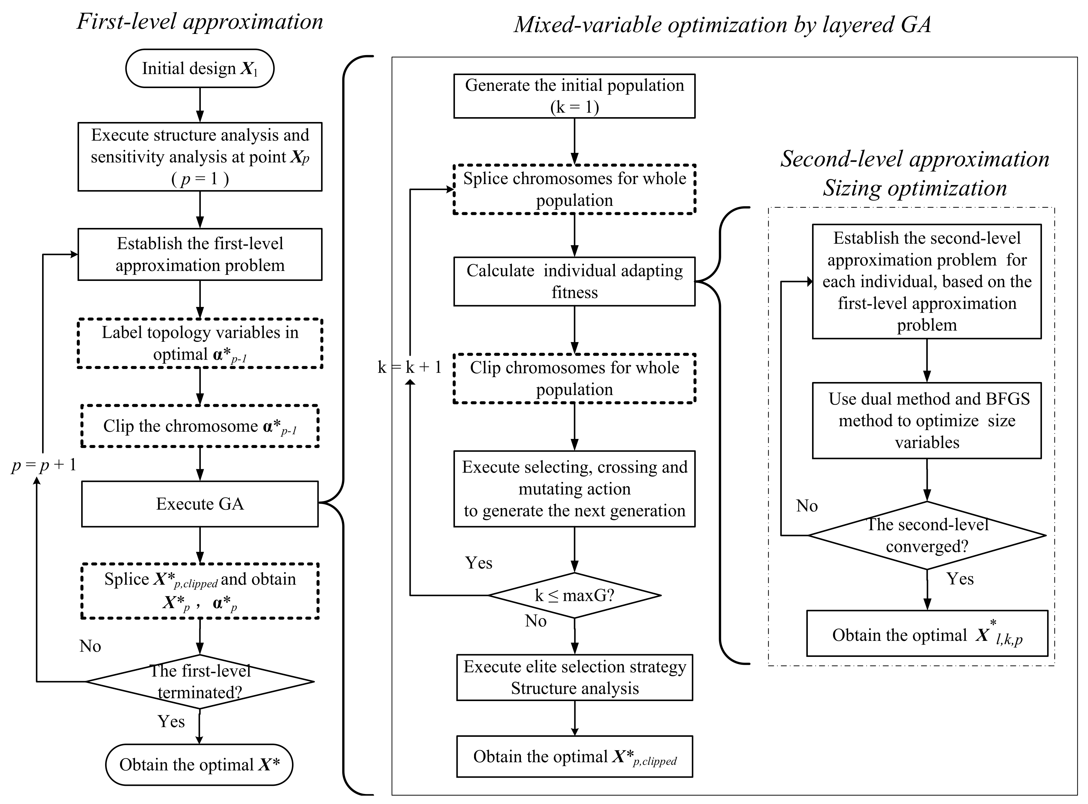
3.1. Flowchart for the Optimization Scheme

The flowchart of a hierarchical optimization scheme for large-scale truss sizing and topology optimization is shown in Figure 2. Before optimizing the mixed variables by GA, a first-level approximation problem is established by the BMA method. As the state of the model, the current optimal variable contains a size vector X p * and topology vector α p * coded in the GA chromosome. The current optimal α p * chromosome is then labeled and clipped. To solve for different types of design variables, GA is nested with an internal optimization, as shown in the dotted box. In an external GA, topology variable vectors are binary-coded to form individuals, and a certain number of individuals make up a population. The initial population is generated based on the current best individual clipped, while all the individuals are only spliced at the validity check and in the fitness calculation. Based on the given value of the topology variable vector, truss cross-sectional sizes for each member in the k-th population are determined through internal optimization. To determine the optimal size of this topology design, the Taylor expansion approximation is conducted based on the first-level approximate functions, and then the dual method and BFGS method are used to solve it. On the basis of the optimal results of internal optimization, the fitness value of each individual can be obtained. After the end of the GA iteration, the current optimal design variable X p * , α p * is obtained through elite selection based on structural analysis. It updates the first-level approximation problem as a new point is added, and the whole algorithm goes to the next p + 1 iteration. Structural analyses and sensitivity analyses are implemented in the general finite element analysis software MSC.PATRAN/NASTRAN, while the two-level approximation and the GA and size optimization are implemented by the FORTRAN program. The Patran Command Language (PCL) is utilized for software calculation and programming optimization to realize the automation of a series of complex processes.

3.2. The First-Level Approximation Problems by BMA

The branched multipoint approximation (BMA) method has proven to be one of the most effective approximation techniques for complicated structure optimization problems [26] and is applied to approximate functions of the primal problem in Equation (1). The function g j X , α is approximated as g j p X , α in Equations (2)–(6). In the p-th stage, g j p X , α is the j-th approximate constraint function at the p-th stage.
g j ( p ) X , α = t = p ( H 1 ) H g j X t , α t + i = 1 n g ˜ j , i , t X , α h t X , α
g ˜ j , i , t X , α = 1 r o , t g j X t , α t x i x i t 1 r o , t x i r o , t x i t r o , t ,   i f   α i = 1 1 r m , t g j X t , α t x i 1 e r m , t x i x i t ,   i f   α i = 0
h t X , α   = h ¯ t X , α i = 1 H h ¯ l X , α t = 1 , , H
h ¯ l X , α = s = 1 , s l H X X s T X X s
min z = 1 H g j X z , α z g j X t , α t g ˜ j , i , t X t , α t 2 s . t .    5 r o , t 5 ,    5 r m , t 5 ,    t = 1 , , H 1
where x t is the t-th known point (from structural analyses), H is the number of counted points in the approximate function, and H = min p , H max . When the number of known points is larger than H max (in this work, H max = 5 ), only the last H max points are included in the function. X ¯ is the convex domain that limits the bounds of x ; h t X , α is a weighting function, which is defined in Equations (4) and (5). r o , t and r m , t are the adaptive parameters controlling the nonlinearity of g j p X , α , which are determined by solving the least-squares parameter estimation in Equation (6). Here, g j X z , α z is the j-th constraint value of the t-th known point. For every value of t, a parameter r t ( r o , t or r m , t ) will be obtained from Equation (6). To avoid large fluctuations in the approximation formula, the value range of r t ( r o , t or r m , t ) should be limited to within (−5, 5). If t equals 1, then r o , t = 1 and r m , t = 3.5 . It can be seen that the construction of the approximate function only requires the partial derivatives of the continuous variables, and discrete variables only act the role of branching, deciding α1 to equate to which value, i.e., 0 or 1. The form of the BMA function is similar to the Hermite interpolation function, and in the known points, the value of the approximate function and their derivatives are consistent with the values in the primal function. This approximate function has been proven to be efficient without singularity even if the continuous variables are close to zero. The approximation accuracy of BMA functions was discussed in [27,28].
To solve the problem in Equation (1), which is always implicit and nonlinear, a first-level approximation problem is first constructed to transform it into an explicit problem. Based on the above BMA method, the first-level approximation problem in the p-th stage is:
{ F i n d      X p = { x 1 ( p ) , x 2 ( p ) , , x n ( p ) } T               α = { α 1 ( p ) , α 2 ( p ) , , α n ( p ) } T M i n      W ( p ) ( X p , α p ) = i = 1 n α i ( p ) W i ( x i ( p ) ) S . t .        g j ( p ) ( X p , α p ) 0                                    j = 1 J 1              α i ( p ) x i ( p ) L + ( 1 α i ( p ) ) x i b x i ( p )              x i ( p ) α i ( p ) x i ( p ) U + ( 1 α i ( p ) ) x i b              α i ( p ) = 0      o r      α i ( p ) = 1                         i = 1 n
x i p U = min x i U , x ˜ i p U
x i p L = max x i L , x ˜ i p L
where g j p X , α is the approximate constraint function and W p X , α is the objective function at the p-th stage. J 1 is the number of active constraints related to the primal problem in Equation (1). x i p U and x i p L are the upper and lower bounds of x i at the p-th stage; x ˜ i ( m ) U x ˜ i p U and x ˜ i p L are the moving limits of x i at the p-th stage.
In the p-th stage of optimization, the optimal result, as a new point, in the p-1-th stage is added to update the approximate functions. The data of the initial first point is deleted; thus, the number of counted points in the approximate function remains constant in the iteration of the first-level approximation problem. Since the first-level approximation problem involves both continuous and discrete variables, it can never be solved directly by using general mathematical programming methods. If GA is directly used and the continuous and discrete variables are encoded simultaneously, the scale of the design variables and the computational costs will become tremendous. Thus, a layered optimization strategy is introduced: discrete variables are optimized by GA in the external layer, and continuous variables are optimized in the internal layer by using the dual method, which can significantly reduce the gene code length in GA while improving the optimization efficiency and accuracy.

3.3. The Label–Clip–Slice Strategy and GA to Address Mixed Variables

The BMA is a method of local approximation and has an effective range for design variables. The farther the point is from the known point constructing the approximation, the worse the approximation is at this point. In addition, the search domain of GA expands exponentially as the topology variables increase based on binary encoding. Thus, for a large-scale truss, the variation of 0/1 topology variables in GA with respect to the last optimal result in the last iteration of the first-level approximation problem becomes extremely large. In other words, the point to approximate in BMA would be far away from the known points that construct the approximation. This will cause the accuracy of the approximation to greatly decrease. The search will then become almost random and will lose the right search direction, which is fatal for optimization in a huge search domain. Therefore, the label–clip–splice strategy (LCS) is proposed to reduce this size contrast. It contains three parts: label the topology variables, clip the chromosomes and splice the chromosomes and is nested on the optimization scheme.

3.3.1. Labeling of the Topology Variables

As shown in Figure 3, for the optimal individual in the last iteration of the first-level approximation problem, we save and inspect its code, which is the topology variable of the optimal structure. When the bits of code are “0” for continuous k generations, their bit orders are labeled as R b i t . Here, k is a control parameter in this strategy and needs an appropriate value. If k is too large, GA labels few variables after many iterations. Moreover, it is very likely to not label any variable for dozens of iterations due to the large search domain and GA operators. If k is too small, many variables will be quickly labeled within a few iterations, and the number will increase with more iterations. The GA will quickly converge to a local optimum, which is far from the global optimum. Hence, the value of k for a specific problem needs to be appropriate but not fixed, similar to other parameters in GA. Its appropriate value pertains to the characteristics of the specific problem to address.

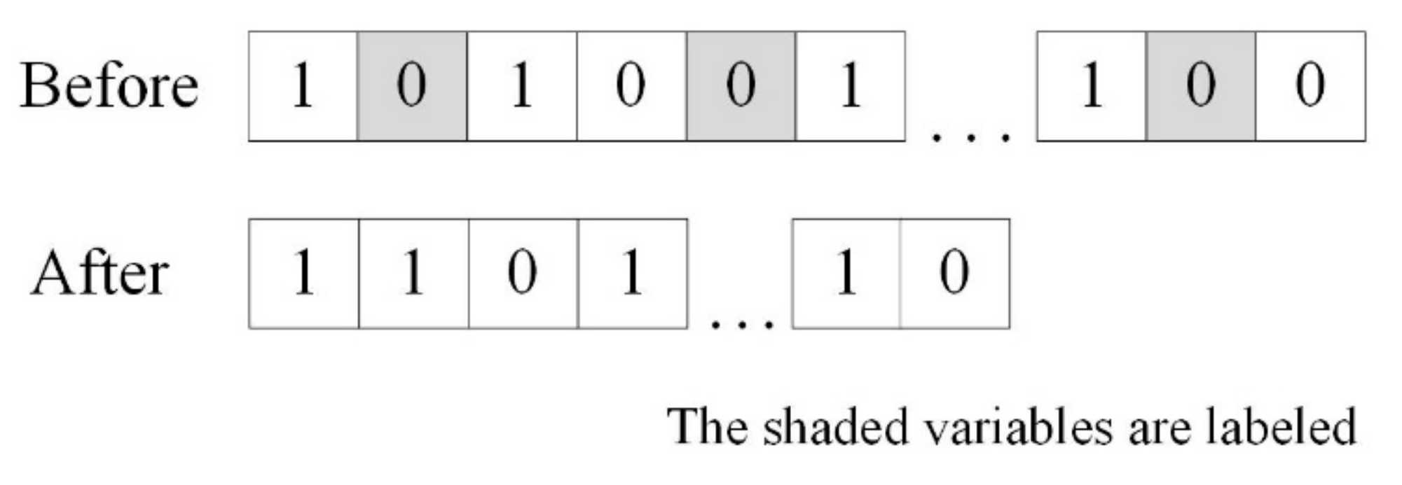
3.3.2. Clipping of the Chromosome of the Last Best Individual

In the next iteration, the optimal individual of the last iteration that has been labeled is first clipped before executing GA optimization. As shown in Figure 3, the shaded variables that have been labeled are clipped, and a new individual with a shorter chromosome is reassembled by the remaining topology variables in sequence. The following steps, including “generate the new population”, “crossover”, and “mutation”, are all carried out in individuals with this shorter chromosome length. In other words, the labeled topology variables are not involved in these processes and remain at “0”.

3.3.3. Generating of the Initial Population

Based on the vector α p 1 , c l i p p e d * , which has been clipped from the vector α p 1 * obtained in the last iteration, the GA generates a random initial population, in which the vector α l , k , p = α l , k , p , 1 , , α l , k , p , n T k = 1 represents the l-th individual in the k-th generation at the p-th iteration of the first-level approximation problem. The initial population consists of three parts:
(a)
The optimized individual α p 1 , c l i p p e d * that is obtained in previous iterations;
(b)
Individuals that randomly mutated from the optimized topology vector α p 1 , c l i p p e d * ;
(c)
Individuals that are calculated according to the optimized size vector X p 1 , c l i p p e d * .

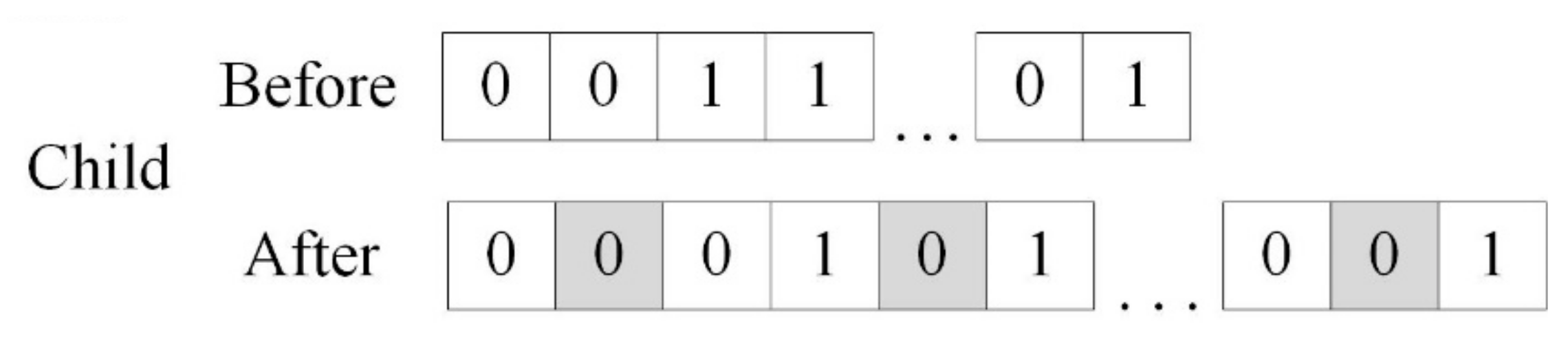
3.3.4. Splicing of the Individuals in the Current Population

In the iterative process, the variables labeled R b i t are spliced to their original positions for the above population before checking the validity of the structure configuration and calculating the individuals’ fitness. In the two stages, the topology variables will not be operated on but the size variables will be. The shaded bits are the label variables, and they are spliced to each individual, as shown in Figure 4. This is because the validity check needs the individual’s physical meaning, which consists of all the initial variables. In addition, the labeled variables have almost no effect on the fitness calculation of GA.

3.3.5. Fitness Calculation and Sizing Optimization

Before calculating the fitness of each individual, the validity of the topology configuration is checked. Invalid individuals are set to a small fitness value and will not be considered by the GA. Considering the mixed variables, the individual fitness is calculated with a penalty function method based on the formulations defined in Equations (10)–(14).
f i t n e s s ( X l , k , p * , α l , k , p ) = f max p W p X l , k , p * , α l , k , p + p e n a l X l , k , p * , α l , k , p
f max p = max l = 1 , 2 , , N s W p X l , k , p * , α l , k , p + p e n a l X l , k , p * , α l , k , p
p e n a l X l , k , p * , α l , k , p = W ¯ j = 1 J 1 g ¯ j j = 1 J 1 g ¯ j 2 v j X l , k , p * , α l , k , p
v j X l , k , p * , α l , k , p = max 0 , g j p X l , k , p * , α l , k , p
W ¯ = 1 N s l = 1 N s W p X l , k , p * , α l , k , p   g ¯ j = 1 N s l = 1 N s g j p X l , k , p * , α l , k , p v ¯ j = 1 N s l = 1 N s v j X l , k , p * , α l , k , p
The above formulas describe the f i t n e s s X l , k , p * , α l , k , p calculation of the l-th individual in k generation of GA for the p-th stage of the first-level approximation problem. X l , k , p * is the optimum size variable vector; α l , k , p is the topology variables of the l-th individual; f max p is the maximum fitness value among all individuals; and W p X l , k , p is the objective value. J 1 is the number of active constraints; N s is the number of valid individuals in the present population; W ¯ is the average weight of these individuals; g j p X l , k , p * , α l , k , p is the approximate constraint functions calculated with the formulations defined in Equations (2)–(6); g ¯ j is the average of g j p X l , k , p * , α l , k , p ; v j X l , k , p * , α l , k , p is the violation level of the j-th constraint for the l-th individual; and v ¯ j denotes the average of v j X l , k , p * , α l , k , p . The optimum size variable vector X l , k , p * is obtained by solving a second-level approximation problem. In the m-th step, the second-level approximation problem is given by Equation (15):
{ f i n d     X ˜ = { x ˜ 1 , , x ˜ n } M i n    W ˜ ( m ) ( X ˜ , α l ) = W ( p ) ( X ˜ ( m ) , α l ) + i = 1 D W ( p ) ( X ˜ ( m ) , α l ) x ˜ i ( x ˜ i x ˜ i ( m ) ) s . t .       g ˜ j ( m ) ( X ˜ , α l ) = g j ( p ) ( X ˜ ( m ) , α l ) i = 1 D x ˜ i ( m ) 2 g j ( p ) ( X ˜ ( m ) , α l ) x ˜ i ( 1 x ˜ i 1 x ˜ i ( m ) ) 0      j = 1 , , J 2            x ¯ i ( m ) L x ˜ i x ¯ i ( m ) U                                                                                          i = 1 , , n x ¯ i ( m ) L = min { x i ( p ) L , x ˜ i ( m ) L } x ¯ i ( m ) U = max { x i ( p ) U , x ¯ i ( m ) U }
where W ˜ ( m ) X ˜ , α l is the approximate objective value obtained by the first-order Taylor expansion of design variables in the m-th step, g ˜ j ( m ) X ˜ , α l is the approximate value of the j-th constraint obtained by the first-order Taylor expansion of reciprocal design variables in the m-th step, x ˜ i ( m ) U and x ˜ i ( m ) L are move limits of x ˜ i in the m-th step. x ¯ i ( m ) U and x ¯ i ( m ) L are the upper and lower bounds of variables x ˜ i . After the construction of the second-level approximation problem, a dual method is implemented to transform the constraint optimization problem into an unconstrained problem. Then, an unconstrained optimization algorithm BFGS is used to seek the optimization size variable X l , k , p * .
After fitness calculation and obtainment of the optimal size results, the labeled bits for all individuals are clipped again before conducting the genetic roulette wheel selection, crossover, and mutation operator procedures in sequence due to their only processing topology variables. When the maximum generation is reached in every run of the GA, it goes to the elite selection strategy. A few (i.e., 5) appropriate individuals (the individual with the highest fitness value and four individuals of the lowest weight) are selected. Among them, the individual X p , c l i p * that satisfies the constraints will be selected as the elite individual and reserved for the next generation.
x i p x i ( p 1 ) ε x     i = 1 , 2 , , n   Max g 1 p X p , α p , g 2 p X p , α p , , g J 1 p X p , α p ε g o r p p max W p X p , α p W p X p 1 , α p 1 W p X p , α p ε f
The convergence criterion defined in Equation (16) is used to determine whether the first-level approximation problem is terminated, as well as the whole scheme. ε x is the convergence control parameter of size variables, ε g is the constraints control parameter, ε f is the weight convergence control parameter, and p max is the maximum iterative number for the first-level approximation problem. In this paper, ε x = 0 . 0001 , ε g = 0.05 , ε f = 0.001 , and p max = 100 ; the maximum number of second-level iterations for sizing optimization is 20 with a convergence accuracy of 0.001.

3.4. Analysis and Discussion

The label–clip–splice strategy is proposed to solve the problem of the large search domain of GA resulting in the bad approximation effect of BMA for large-scale truss optimization. Its efficacy is analyzed and discussed from the understanding of the problem without the LCS strategy.
The number of whole topology variables is set as n , and the topology variable α = α 1 , α 2 , , α n ; then, the total search domain of topology variables in the current iteration for the GA is Ω = 2n. Here, the iteration means the solution process of the first-level approximation problem. m is denoted as the maximum number of topology variables changed with respect to the last iteration’s optimal result after a GA process. Obviously, m increases when n becomes bigger. This means that the two optimal topology variables between two consecutive iterations are very different for large-scale problems. In other words, the new updated points will be far away from the known points that construct the first-level approximation problem. The accuracy of approximation will decrease with more iterations. As a result, the GA will search with very inaccurate functions, wander locally in a huge domain and lose the right direction for optimization. A more serious result is that the iteration will diverge. The former result is illustrated schematically in Figure 5. The global optimum x is marked by a red point. The purple area indicates a distribution domain Ωi of some optimum individuals in the GA of each iteration, and the yellow area indicates a total search domain Ω. Owing to the inaccuracy of approximation caused by large-scale variables of GA, the optimization scheme without the LCS strategy is almost impossible to catch x in Ωi (i = 1, 2, …, n), as shown in the Figure 5.
The LCS technique shrinks the search domain by decreasing the dimensions of topology variables. The optimal result is saved in each iteration. In the p-th iteration of the first-level approximation problem, the last optimal result X p - 1 is inspected after being used in updating the first-level approximation. The position i where α p 1 , i * = 0 is labeled like fluorescent labeling. If some positions i 1 , i 2 , , i q are labeled for k consecutive iterations, the bits of the topology variable α p - 1 , i 1 * , α p - 1 , i 2 * , , α p - 1 , i q * are cut off from individual α p 1 * of the GA. Then, this clipped individual is used to generate the initial population for the GA process in the p-th iteration. Thus, the topology variable’s dimension involved in GA optimization is reduced empirically in this way, and the search domain is shrunk at an exponential speed Ω p = 2 n q . This will decrease the distance between approximate points and maintain a sufficiently good approximation accuracy, which offers an appropriate search direction in a large search domain. As shown schematically in Figure 6, the purple and yellow areas have the same meaning as Figure 5. The domain bounded by a red circular curve is Ω p , which indicates the search space that has shrunk in each iteration. As the optimization iterates, the total search domain decreases gradually so that the bad effect on the accuracy of BMA will be weakened. With an accurate result of BMA for GA, the optimization can go along the right way and would eventually catch x in Ω i afterward.

4. Numerical Examples

Numerical examples are presented in this section to illustrate the feasibility of the proposed method in handling large-scale truss optimization problems with size and topology design variables. First, its effectiveness and efficiency are verified by designing a classic small-scale truss structure, and a brief comparison with the literature is made. Subsequently, the structure of a large-scale cantilever truss is optimized to show the effectiveness of the LCS strategy on a large-scale problem by contrast with the scheme without the LCS strategy. Afterward, the efficacy of the improved scheme on large-scale truss optimization is verified by a large-scale Michell truss problem with mixed variables. Comparison of the same-scale problem with other literature results demonstrates its high efficiency with very few structural analyses.

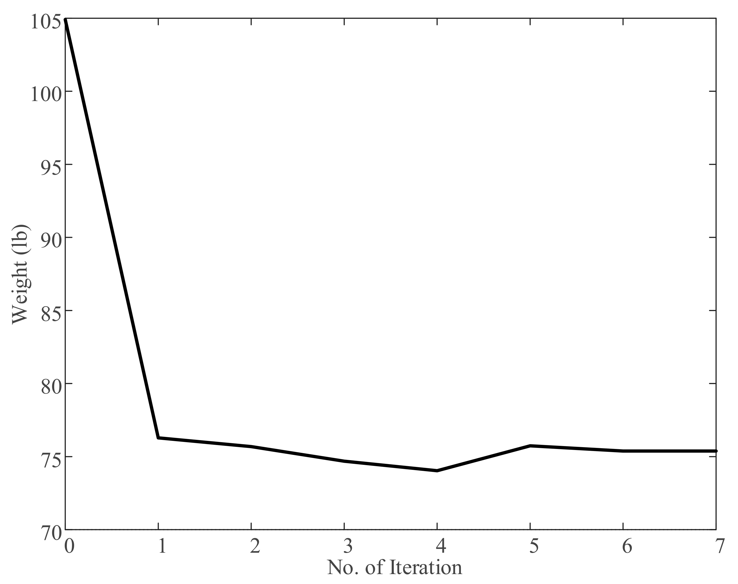
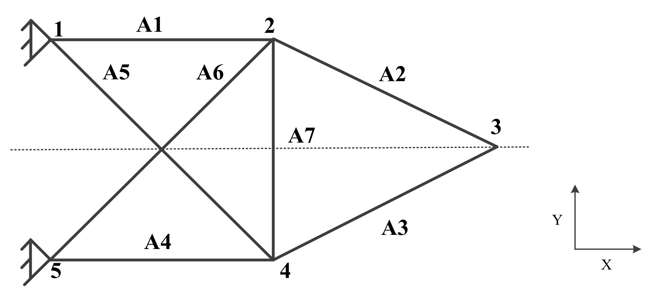
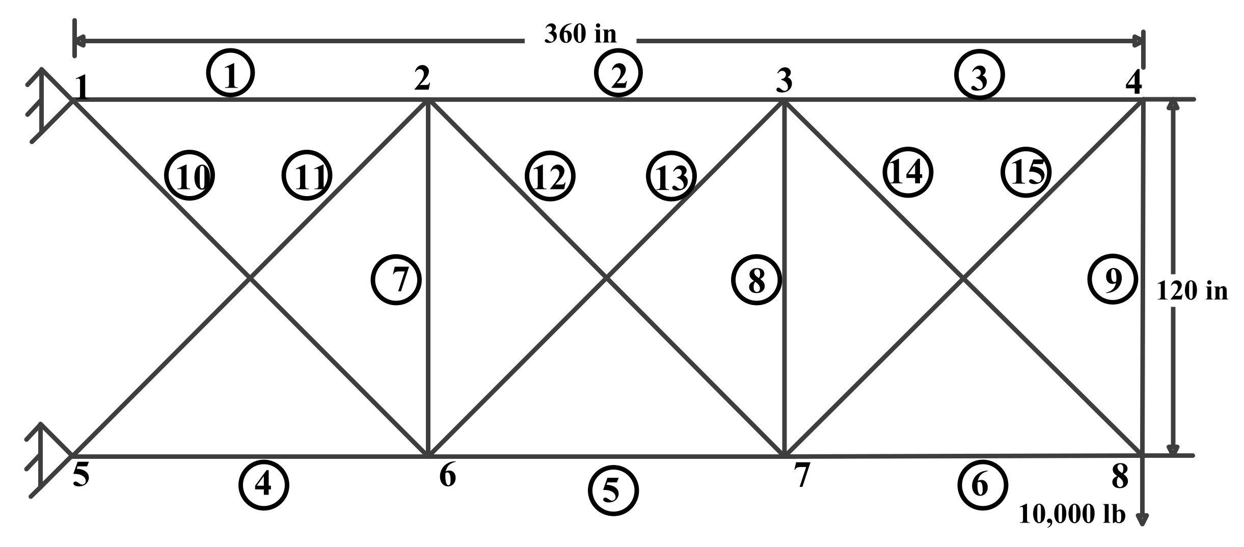
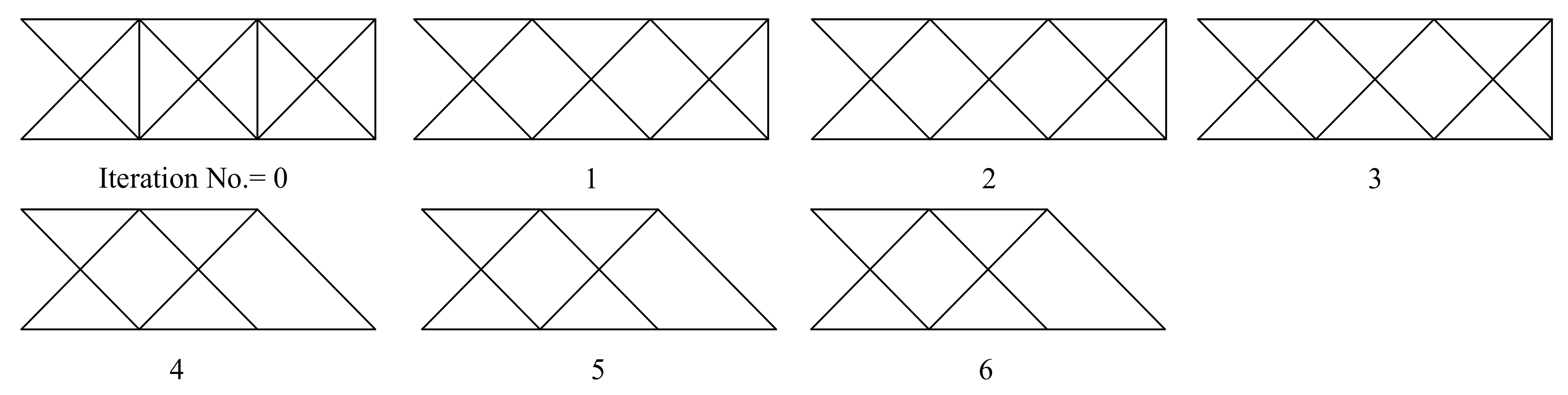
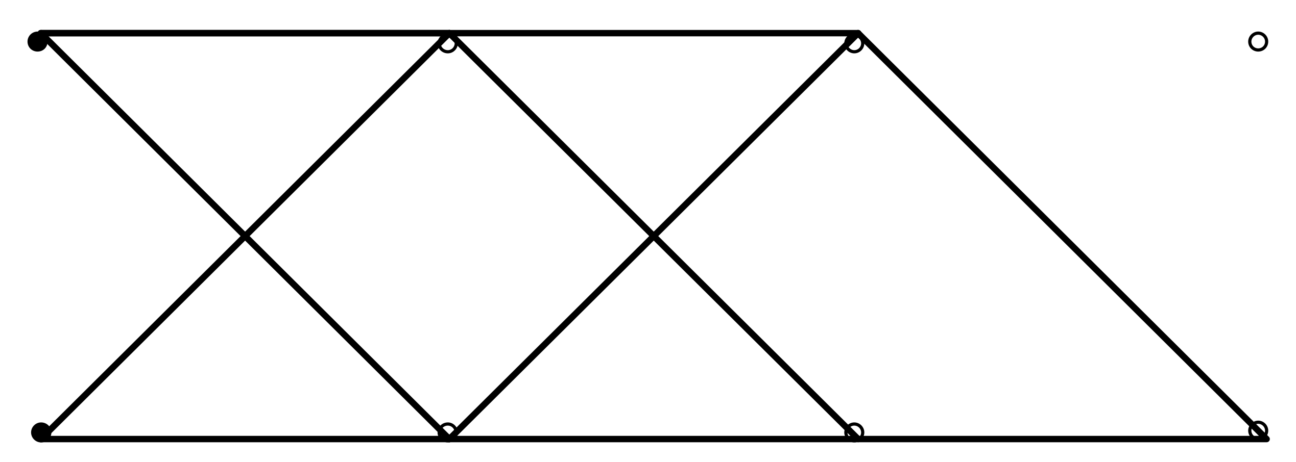
4.1. Example 1: 15-Bar Planar Truss

The ground structure of this example is shown in Figure 7. A vertical tip load of 10,000 lb is imposed on node 8. The material density is 0.1 lb/in.3 and Young’s modulus is specified as 1.0 × 10 7 Psi. The weight of this truss is minimized with 15 size variables and 15 topology variables. The original cross-sectional area for each bar is 0.5 in.2 and is permitted to vary from 0.1 in.2 to 10.0 in.2. The stress limit is 25,000 Psi for both the tension and compression of all members. The parameters of the GA are set as follows: the population size is 100, evolution generation is 100, and crossover and mutation probabilities are 0.9 and 0.1, respectively.
Figure 8 illustrates the topology evolution. Two typical configurations are generated in the iterative procedure (Iterations 1 and 4). Figure 9 shows the optimized configurations of this paper, and Figure 10 shows the weight iteration history of this paper. The optimal solutions of variables, structural weight, critical constraint, and structural analyses are listed in Table 2 and compared with the literature. The optimal weight found by this paper is 75.376 kg after seven iterations. In contrast with the 15-bar truss size and layout optimization of previous studies, our solution weighs less than the solutions found by Tang [29], Miguel [30] by 5.57% and 0.23%, respectively. The critical constraint is zero, implying the validity of the presented result. Five topology variables were labeled in the process. In particular, the method in this paper converged by 15 structural analyses. Compared with past studies, this method only took 0.19% of the structural analyses in the referred to literature, demonstrating the greatly enhanced efficiency of the proposed method. The optimal results of this classic example and the comparison illustrate the efficacy and the high efficiency of the improved method on truss optimization with mixed variables.

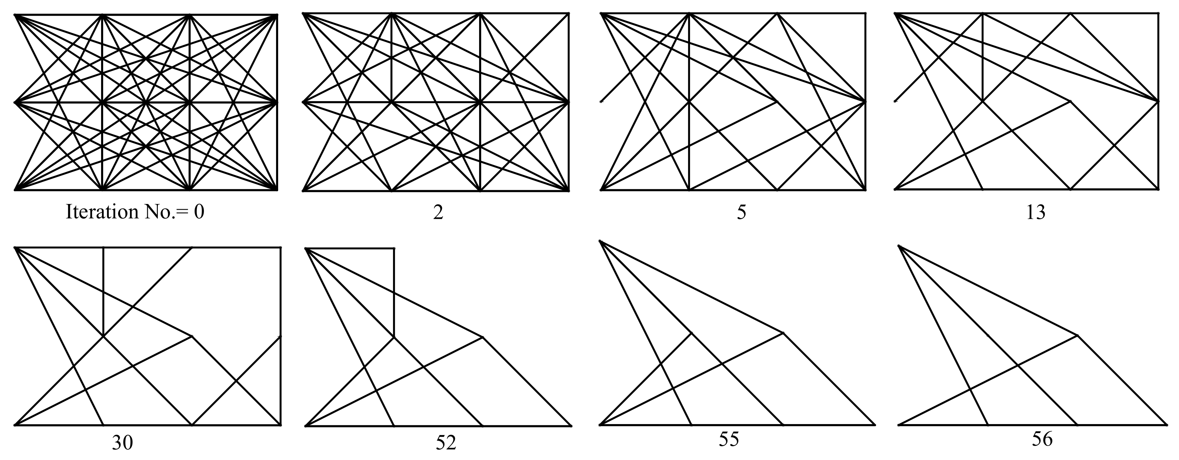
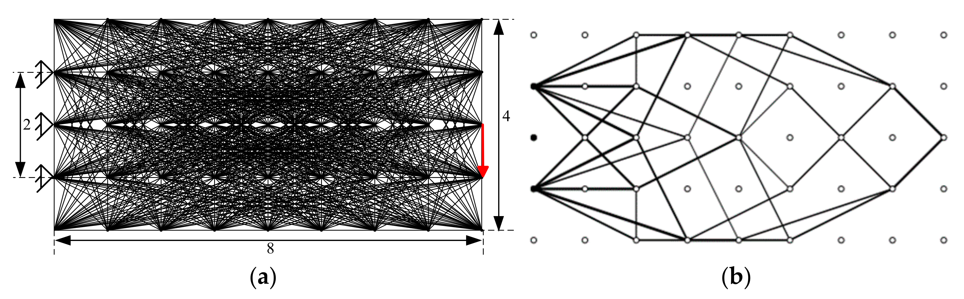
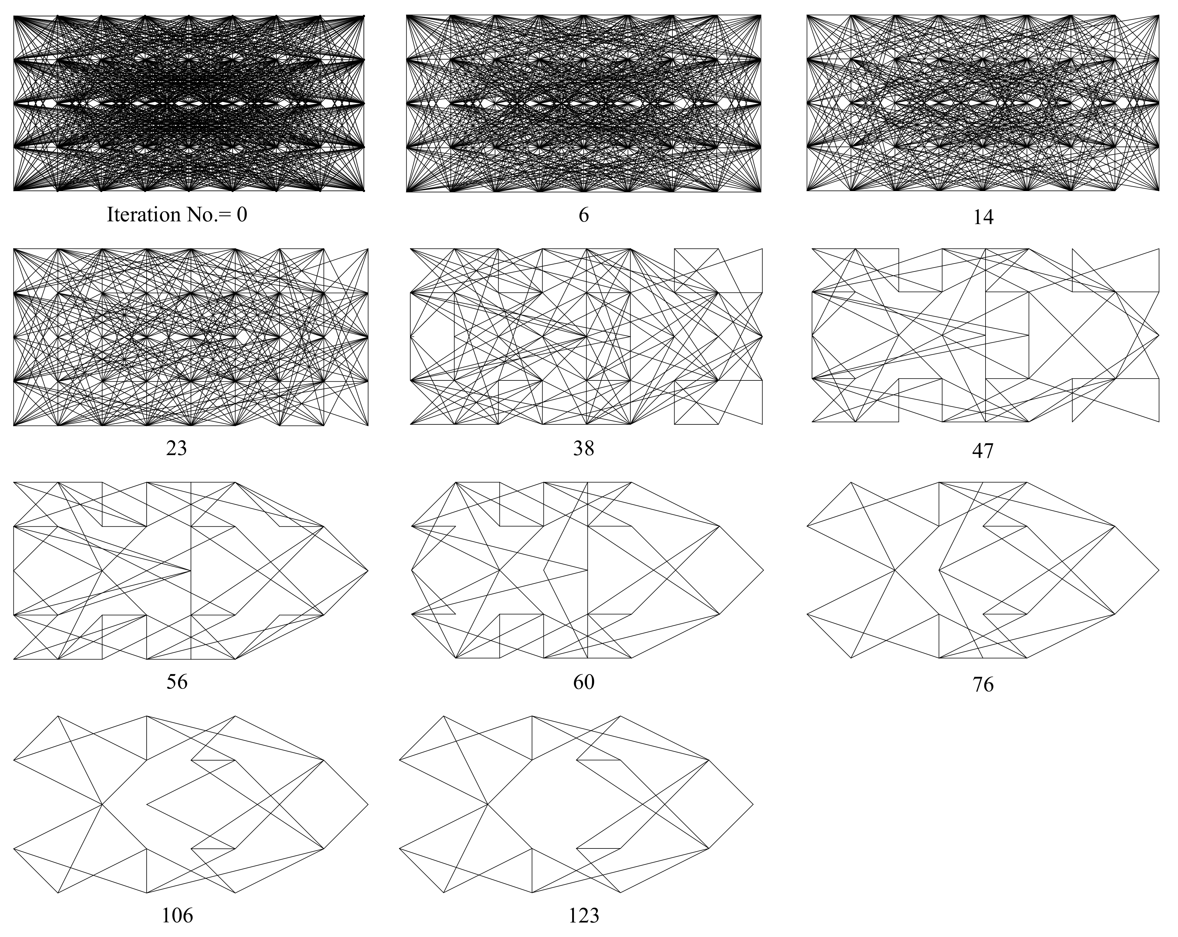
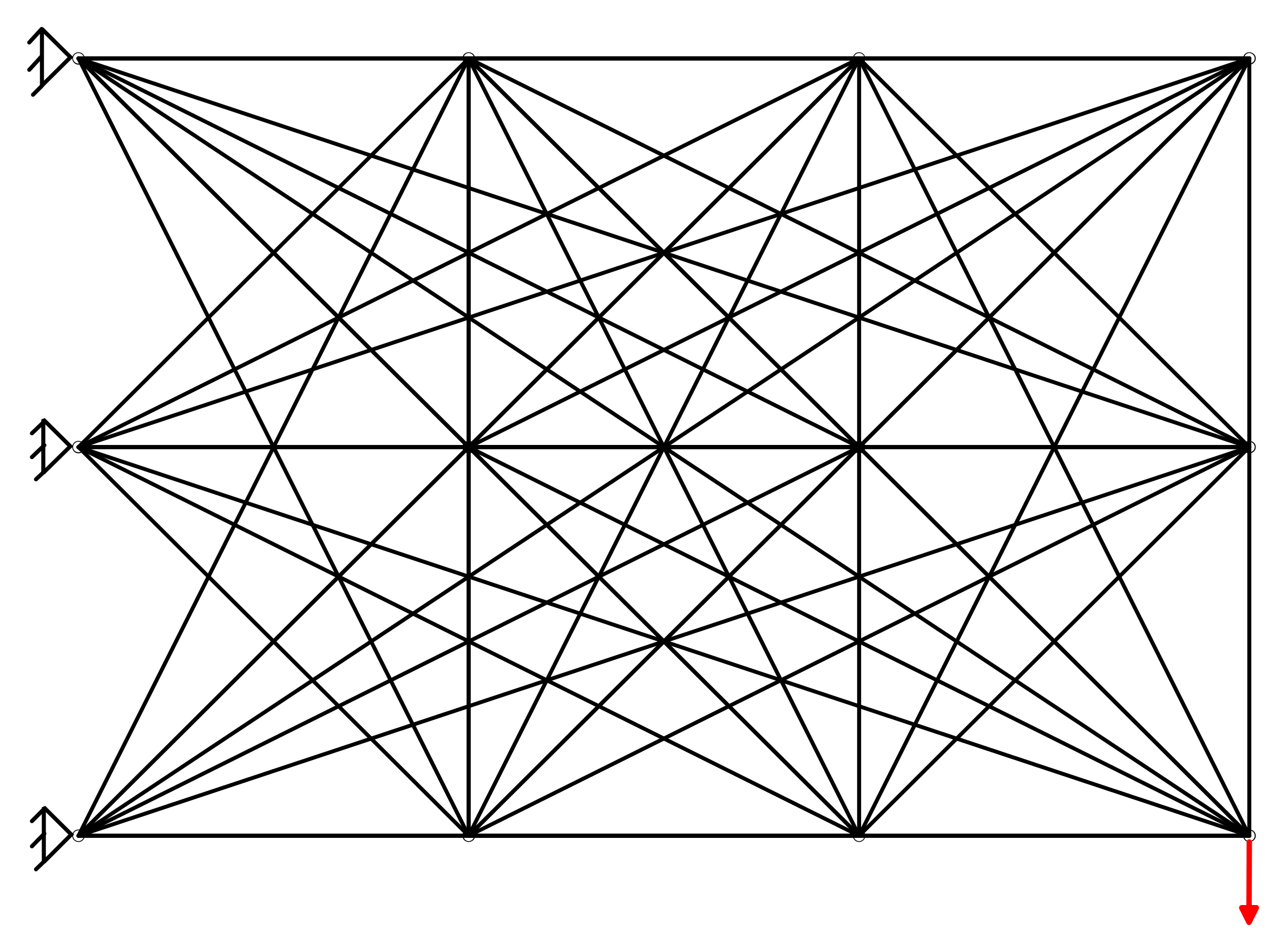
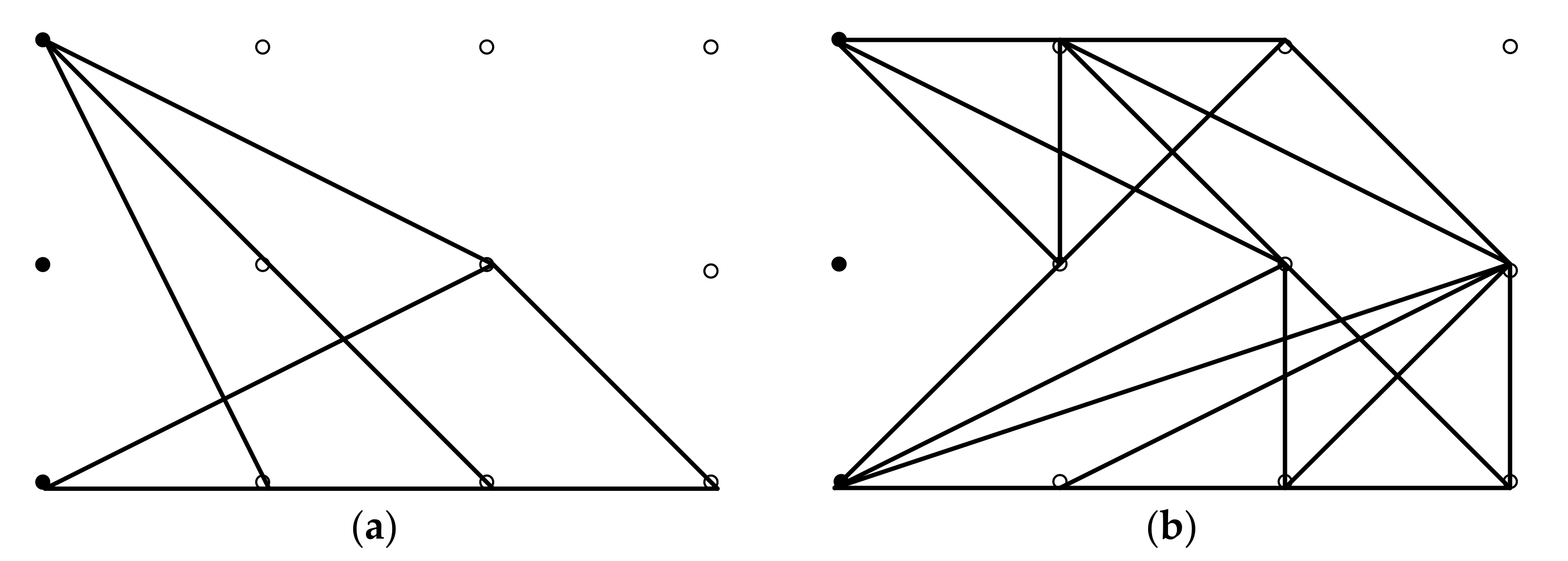
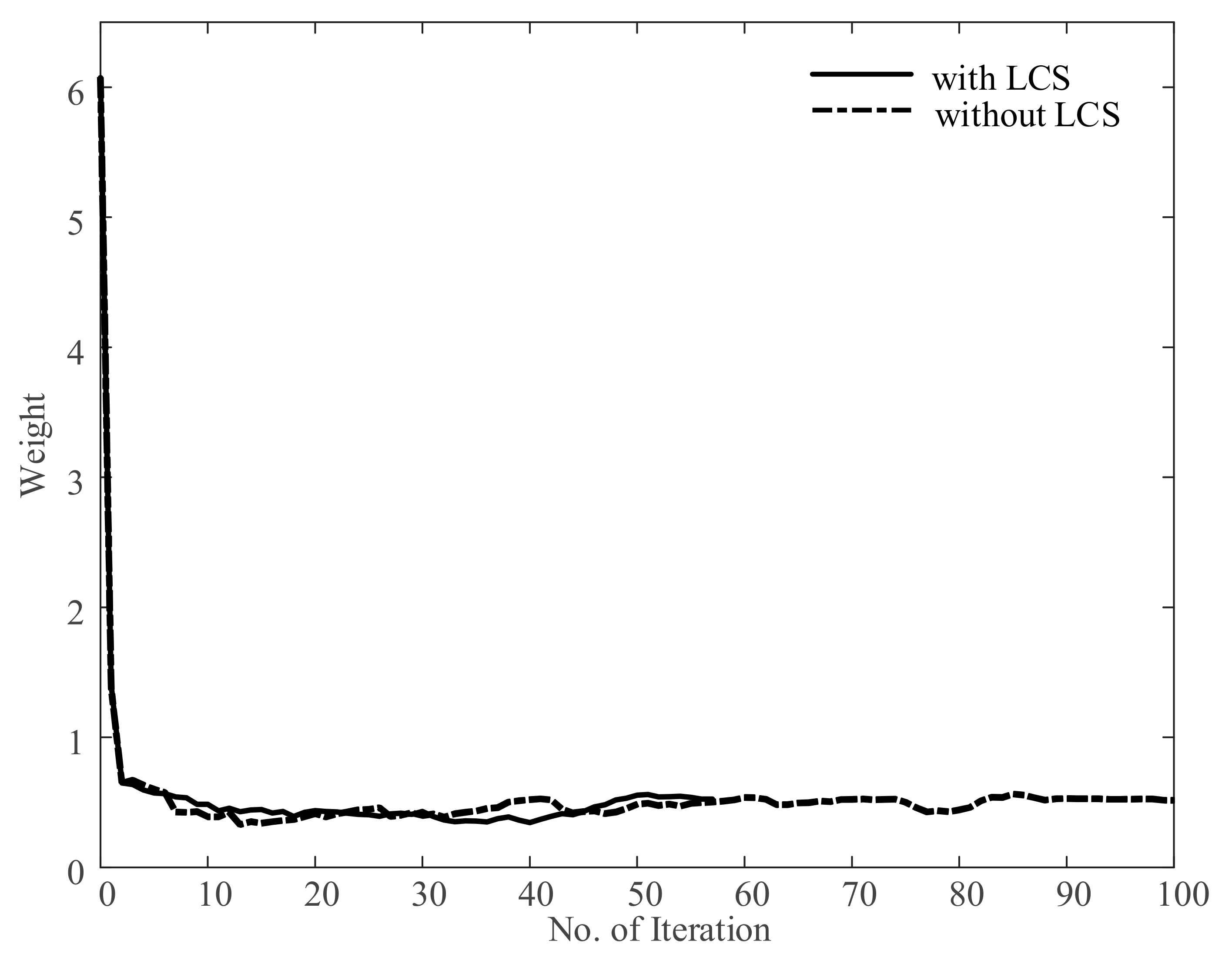
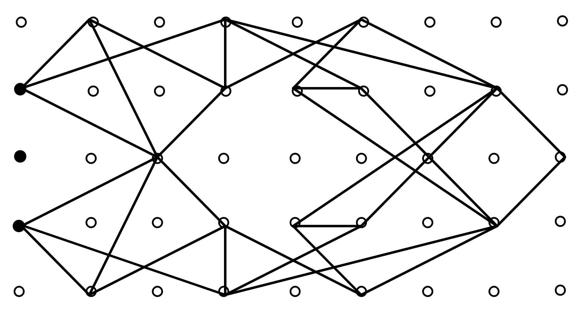
4.2. Example 2: A Cantilever Truss

A large-scale cantilever truss is adapted from the numerical example in the research of Wolfgang Achtziger and Mathias Stolpe [31]. As shown in Figure 11, this cantilever truss has 63 bars. The width and height of the rectangular truss are 3 and 2, respectively. The nodes on the left side are pinned, and a vertical external load is applied at the bottom of the right-hand side that equals 1. Nodes are connected by a potential bar unless this creates an overlapping bar. The density is 1, and the modulus of elasticity is 1000. The original cross-sectional area for each bar is 0.1 and is permitted to vary from 0.01 to 10. The nodal displacement of the loading point is limited from −0.05 to 0.01. The parameters of GA are set as follows: the population size is 150, the maximum number of evolutions is 100, and the initial probabilities of crossover and mutation are 0.9 and 0.1, respectively.
Figure 12 illustrates the topology evolution. Gradually changing configurations are generated in the iterative procedure, and eight typical configurations are chosen. Figure 13 shows the optimized configurations of this paper compared with the same method without the LCS strategy, and the weight iteration history for the two methods is presented in Figure 14. The method without the LCS strategy yields a result of nonconvergence and a middle topology configuration, and the method with the LCS strategy obtains a more concise, effective, and valid configuration. The optimal solutions of variables, structural weight, critical constraint, and structural analyses are compared in Table 3 and Table 4. The critical constraint of the method without the LCS strategy is 5.492 × 10⁻², which indicates the iteration’s nonconvergence. The method with the LCS strategy converges after 57 iterations and 66 analyses with 51 topology variables labeled, showing the efficiency of the proposed method. The contrast of the two circumstances verifies the efficacy and efficiency of the LCS strategy in improving the GA with BMA on addressing the size and topology optimization for large-scale trusses with mixed variables.

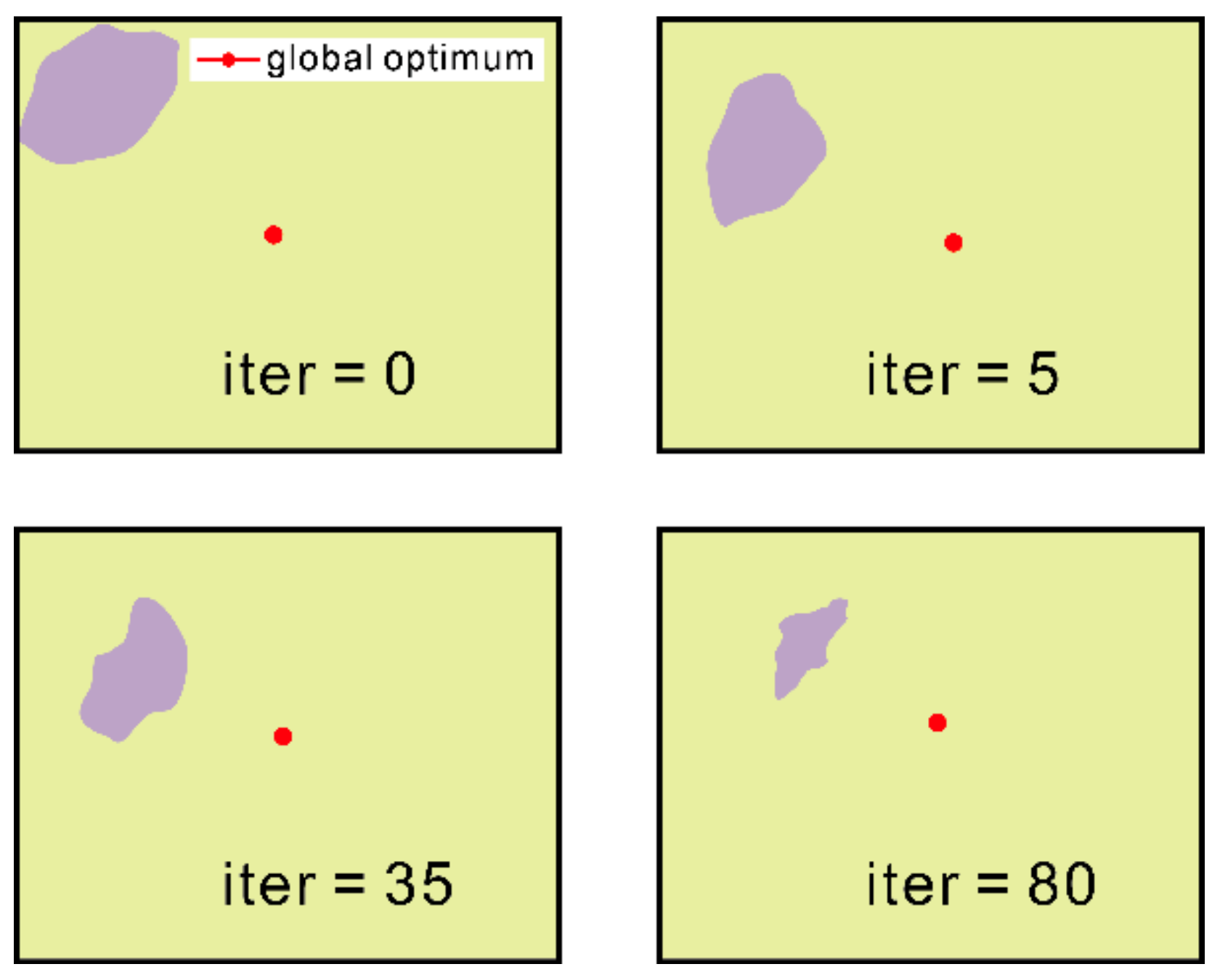
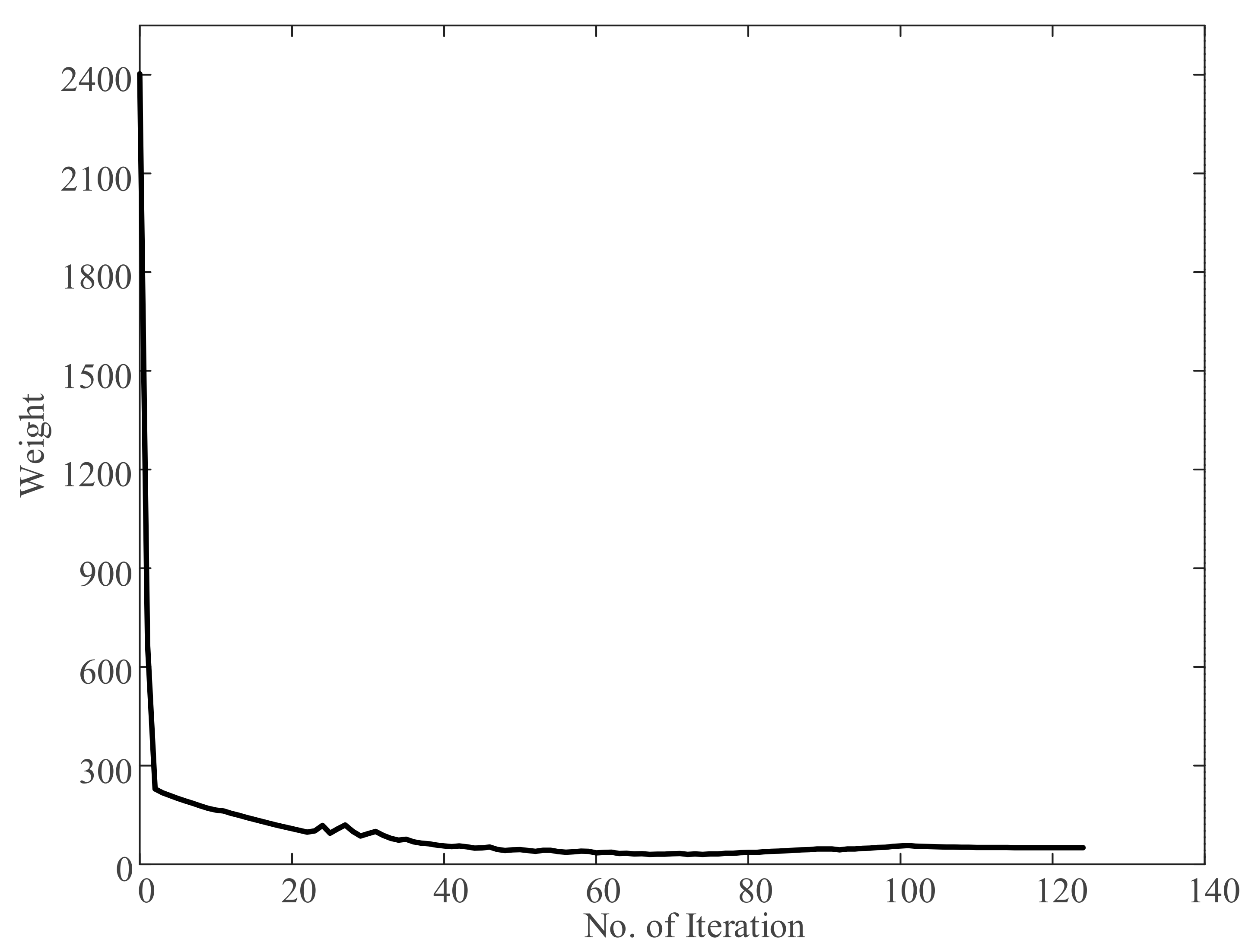
4.3. Example 3: A Michell Truss

The ground structure for the 662-bar Michell truss shown in Figure 15a was studied by Wolfgang Achtziger and Mathias Stolpe [31,32]. The data are consistent with the literature. The width and height of the whole structure are 8 and 4, respectively. Three nodes on the left side, centered on the horizontal mid-axis, are fixed to a rigid wall of height 2, these are indicated as filled (“•”), and other nodes that are not filled (“◦”) are free. Nodes are connected by a potential bar unless this creates an overlapping bar.
In the referred literature, the modulus of elasticity is 1, and the cross-sectional area is chosen from the set {0, 1} for all bars. The objective function is the minimum strain energy, and the constraint function is a certain volume. The design size variable is discretized into a 0/1 variable, and a series of nonconvex continuous relaxations based on convergent branch and bound algorithms is used to address discrete truss variables. The referred literature achieved topology optimization for this large-scale truss by discrete size variable optimization. The optimum configurations of the work of Wolfgang Achtziger is showed in Figure 15b.
We apply this example to our problem to optimize the size and topology for a large-scale truss with a nodal displacement constraint of the loading point and minimum weight objective. The structural parameters are set as follows: the modulus of elasticity is 103; the density is 1; the load P y = 1 ; the nodal displacement of the loading point is limited from −0.0453 to 0.0453; the initial cross-sectional area is 1, and it is permitted to vary between 0.0001 and 2. The parameters of GA are set as follows: the population size is 100, the maximum number of evolutions is 30, and the initial probabilities of crossover and mutation are 0.9 and 0.05, respectively. The maximum of the first-level iteration is 150, and the convergence accuracy is 0.005; the maximum of the second-level iteration for sizing optimization is 20, with a convergence accuracy of 0.05.
Figure 16 illustrates the topology evolution. Gradually changing configurations are generated in the iterative procedure, and 11 typical configurations are chosen. Figure 17 shows the optimum configurations of this paper. The weight iteration history of this paper is presented in Figure 18. Table 5 and Table 6 offer the optimal solutions of variables, structural weight, critical constraint, and structural analysis. The optimal weight found by this paper is 50.522. The critical constraint is zero, implying the validity of the presented result. The optimization process converged by 124 iterations, and a total of 314 topology variables were labeled. In particular, the method in this paper converged by 139 structural analyses, which only took 1.29% of that in the literature. Thus, the method in this paper achieves a valid optimum result and a concise topology configuration with fewer structural analyses. This advantage is significant because truss optimization problems with mixed variables of a similar scale usually require thousands of structural analyses in past literature [31].

5. Conclusions

This paper proposes a new label–clip–splice strategy to improve GA with a multipoint approximation method to realize simultaneous size and topology optimization for large-scale trusses efficiently. A mathematical model with continuous size design variables and discrete topology design variables is established based on the ground structure. A branched multipoint approximation is used for implicit functions in the model to conduct the first-level approximation problem. GA is selected to address the mixed variables optimization. To solve the problem of a large number of topology variables for GA resulting in a decrease in the approximation effect for BMA and convergence difficulties for large-scale truss optimization, a label–clip–splice strategy is proposed to shrink the search domain gradually and reasonably with iterations.
In addition to verifying the improvement of the label–clip–splice strategy on the hybrid method of GA with BMA for large-scale truss optimization, the numerical simulations in this paper also suggest the efficacy of the presented approach in finding the optimal design of large-scale truss optimization with mixed variables. The performance of the proposed method in reducing the number of structural analyses is significant and is far superior to other methods. Furthermore, the proposed method shows its potential applicability for the optimum design of practical structures with the extensive ground structure method and structural analyses from the finite element method.

Author Contributions

Conceptualization, T.D.; methodology, T.D. and H.H.; validation, Z.D.; formal analysis, T.D.; writing—original draft preparation, T.D.; writing—review and editing, T.D. and Z.Y.; supervision, S.C. and C.H.; project administration, S.C. and C.H.; funding acquisition, S.C. and H.H. All authors have read and agreed to the published version of the manuscript.

Funding

This research was funded by [the National Natural Science Foundation of China] grant number [11672016].

Conflicts of Interest

The authors declare no conflict of interest.

References

  1. Ma, G.; Gao, B.; Xu, M.; Feng, B. Active Suspension Method and Active Vibration Control of a Hoop Truss Structure. AIAA J. 2018, 56, 1689–1695. [Google Scholar] [CrossRef]
  2. Tian, D.; Jin, L.; Liu, R.; Liu, Z.; Fan, X. Research on the Topological Characteristics of Truss Structure for Large Space Modular Deployable Truss Antenna. In Proceedings of the 2020 IEEE 3rd International Conference on Electronics Technology (ICET), Chengdu, China, 8–12 May 2020. [Google Scholar]
  3. Zuo, W.; Saitou, K. Multi-material topology optimization using ordered SIMP interpolation. Struct. Multidiscip. Optim. 2017, 5, 477–491. [Google Scholar] [CrossRef]
  4. Wang, M.Y.; Wang, X.M.; Guo, D.M. A level set method for structural topology optimization. Comput. Meth. Appl. Mech. Eng. 2003, 192, 227–246. [Google Scholar] [CrossRef]
  5. Deng, S.G.; Krishnan, S. Stress Constrained Thermo-Elastic Topology Optimization with Varying Temperature Fields via Augmented Topological Sensitivity Based Level-Set. Struct. Multi-Discip. Optim. 2017, 56, 1–19. [Google Scholar] [CrossRef]
  6. Xie, Y.M.; Steven, G.P. A simple evolutionary procedure for structural optimization. Comput. Struct. 1993, 49, 885–896. [Google Scholar] [CrossRef]
  7. Yang, X.Y.; Xie, Y.M.; Steven, G.P.; Querin, O.M. Bidirectional Evolutionary Method for Stiffness Optimization. AIAA J. 1999, 37, 1483–14889. [Google Scholar] [CrossRef]
  8. Ajit, P.; David, B.; Ian, A.; Ricky, W.; Richard, H. Hierarchical remeshing strategies with mesh mapping for topology optimization. Int. J. Numer. Methods Eng. 2017, 111, 676–700. [Google Scholar]
  9. Fu, Y.-F.; Rolfe, B.; Chiu, L.N.; Wang, Y.; Huang, X.; Ghabraie, K. SEMDOT: Smooth-edged material distribution for optimizing topology algorithm. Adv. Eng. Softw. 2020, 150, 102921. [Google Scholar] [CrossRef]
  10. Huang, X. On smooth or 0/1 designs of the fixed-mesh element-based topology optimization. Adv. Eng. Softw. 2021, 151, 102942. [Google Scholar] [CrossRef]
  11. Dorn, W. Automatic design of optimal structures. J. De Mec. 1964, 3, 25–52. [Google Scholar]
  12. Erbatur, F.; Al-Hussainy, M.M. Optimum design of frames. Comput. Struct. 1992, 45, 887–891. [Google Scholar] [CrossRef]
  13. Tabak, E.I.; Wright, P.M. Optimality criteria method for building frames. J. Struct. Div. ASCE 1981, 107, 1327–1342. [Google Scholar] [CrossRef]
  14. Saka, M.P. Optimum design of pin-jointed steel structures with practical applications. J. Struct. Eng. ASCE 1990, 116, 2599–2620. [Google Scholar] [CrossRef]
  15. Hajela, P.; Lee, E. Genetic algorithms in truss topological optimization. Int. J. Solids Struct. 1995, 32, 3341–3357. [Google Scholar] [CrossRef]
  16. Gandomi, A.H.; Yang, X.-S.; Alavi, A.H. Cuckoo search algorithm: A metaheuristic approach to solve structural optimization problems. Eng. Comput. 2013, 29, 17–35. [Google Scholar] [CrossRef]
  17. Mirjalili, S.; Gandomi, A.H.; Mirjalili, S.Z.; Saremi, S.; Faris, H.; Mirjalili, S.M. Salp Swarm Algorithm: A bio-inspired optimizer for engineering design problems. Adv. Eng. Softw. 2017, 114, 163–191. [Google Scholar] [CrossRef]
  18. Hasançebi, O.; Kazemzadeh Azad, S. Adaptive dimensional search: A new metaheuristic algorithm for discrete truss sizing optimization. Comput. Struct. 2015, 154, 1–16. [Google Scholar] [CrossRef]
  19. Eusuff, M.; Lansey, K.; Pasha, F. Shuffled frog-leaping algorithm: A memetic meta-heuristic for discrete optimization. Eng. Optim. 2006, 38, 129–154. [Google Scholar] [CrossRef]
  20. Sokó, T. Topology optimization of large-scale trusses using ground structure approach with selective subsets of active bars. In Proceedings of the 19th International Conference on Computer Methods in Mechanics, Warsaw, Poland, 9–12 May 2011. [Google Scholar]
  21. Degertekin, S.O.; Minooei, M.; Santoro, L.; Trentadue, B.; Lamberti, L. Large-Scale Truss-Sizing Optimization with Enhanced Hybrid HS Algorithm. Appl. Sci. 2021, 11, 3270. [Google Scholar] [CrossRef]
  22. Azad, S.K.; Aminbakhsh, S. High-dimensional optimization of large-scale steel truss structures using guided stochastic search. Structures 2021, 33, 1439–1456. [Google Scholar] [CrossRef]
  23. Kaveh, A. Optimum Design of Large-Scale Truss Towers Using Cascade Optimization; Springer International Publishing: Cham, Switzerland, 2017; pp. 281–295. [Google Scholar]
  24. Dong, Y.; Huang, H. Truss topology optimization by using multipoint approximation and GA. Chin. J. Comput. Mech. 2004, 21, 746–751. [Google Scholar]
  25. Chen, S.Y.; Shui, X.F.; Huang, H. Improved genetic algorithm with two-level approximation using shape sensitivities for truss layout optimization. Struct. Multidiscip. Optim. 2016, 55, 1–18. [Google Scholar] [CrossRef]
  26. Huang, H.; An, H.; Ma, H.; Chen, S. An Engineering Method for Complex Structural Optimization Involving Both Size and Topology Design Variables. Int. J. Numer. Methods Eng. 2019, 117, 291–315. [Google Scholar] [CrossRef]
  27. Huang, H.; Ke, W.; Xia, R.W. Numerical accuracy of the multi-point approximation and its application in structural synthesis. In Proceedings of the 7th AIAA/USAF/NASA/ISSMO Symposium on Multidisciplinary Analysis and Optimization, St. Louis, MO, USA, 2–4 September 1998; Available online: https://arc.aiaa.org/doi/pdfplus/10.2514/6.1998-4962 (accessed on 22 August 2012).
  28. Huang, H.; Wang, Y.; Lian, H. Comparisons of several multi-point approximation methods used in structural topology optimization. In Proceedings of the Chinese Conference on Computational Mechanics, Beijing, China, 5–6 December 2003; Volume 1. [Google Scholar]
  29. Tang, W.; Tong, L.; Gu, Y. Improved genetic algorithm for design optimization of truss structures with sizing, shape and topology variables. Int. J. Numer. Methods Eng. 2005, 62, 1737–1762. [Google Scholar] [CrossRef]
  30. Miguel, L.F.F.; Lopez, R.H.; Miguel, L.F.F. Multimodal size, shape, and topology optimisation of truss structures using the Firefly algorithm. Adv. Eng. Softw. 2013, 56, 23–37. [Google Scholar] [CrossRef]
  31. Achtziger, W.; Stolpe, M. Global optimization of truss topology with discrete bar areas—Part II: Implementation and numerical results. Comput. Optim. Appl. 2009, 44, 315–341. [Google Scholar] [CrossRef]
  32. Achtziger, W.; Stolpe, M. Global optimization of truss topology with discrete bar areas—Part I: Theory of relaxed problems. Comput. Optim. Appl. 2008, 40, 247–280. [Google Scholar] [CrossRef]
Figure 1. Seven-bar truss structure.
Applsci 12 00407 g001
Figure 2. Optimization flowchart.
Applsci 12 00407 g002
Figure 3. Clipping of the chromosome of the topology variable.
Applsci 12 00407 g003
Figure 4. Splicing of the chromosome of the topology variable.
Applsci 12 00407 g004
Figure 5. Schematic domain with iterations.
Applsci 12 00407 g005
Figure 6. Schematic domain with iterations by the LCS strategy.
Applsci 12 00407 g006
Figure 7. Ground structure of the 15-bar truss.
Applsci 12 00407 g007
Figure 8. Topology evolution of the 15-bar truss.
Applsci 12 00407 g008
Figure 9. Optimization results in this paper.
Applsci 12 00407 g009
Figure 10. Iteration history for the 15-bar truss.
Applsci 12 00407 g010
Figure 11. Ground structure of the 63-bar truss.
Applsci 12 00407 g011
Figure 12. Topology evolution of the 63-bar truss.
Applsci 12 00407 g012
Figure 13. (a) Optimization results in this paper; (b) Optimization results in this paper without the LCS strategy.
Applsci 12 00407 g013
Figure 14. Iteration history for the 63-bar truss.
Applsci 12 00407 g014
Figure 15. (a) Ground structure of the 662-bar truss; (b) The solution of the literature.
Applsci 12 00407 g015
Figure 16. Topology evolution of the 662-bar truss.
Applsci 12 00407 g016
Figure 17. Optimization results in this paper.
Applsci 12 00407 g017
Figure 18. Iteration history for the 662-bar truss.
Applsci 12 00407 g018
Table 1. Definition of design variables.
Design DomainCross-Sectional TypeTopology VariablesSize Variables
TrussBAR αi (i = 1, 2, 3, 4, 5, 6, 7) xi (i = 1, 2, 3, 4, 5, 6, 7)
Table 2. Optimization results of the 15-bar truss.
Design VariablesData from [29]Data from [30]Present
A11.0810.9541.60
A20.5390.5391.59
A300.1410
A41.0810.9542.39
A50.9540.5390.80
A60.4400.2870.79
A700.1410
A80.14100
A903.8130
A100.2700.4401.13
A110.2700.4400.20
A120.5390.2200.20
A130.1410.2201.13
A140.4400.3471.13
A1500.1410
Iteration number 7
Labeled variables 5
Critical constraint−0.00088−0.06490.000
Weight (lb.)77.8474.3375.376
Percentage difference (%)5.570.23
Structural analysis8000800015
Percentage difference (%)0.190.19
Table 3. Optimization results of the 63-bar truss.
With LCSWithout LCS (No Convergence)
Iteration number56100
Labeled variables51/
Critical constraint0.0005.492 × 10−2
Weight0.5250.517
Structural analysis66117
Table 4. Optimal design of the 63-bar truss.
NO.Area
LCS/No LCS
No.Area
LCS/No LCS
No.Area
LCS/No LCS
10.18300.42931500.14301.0140
200.116–180044–4700
30.41130.2727190.10480.11.3853
40.55750.394220–2600491.41540.1386
50.40560.134927–2800.150–5100
600.129–35005200.1
7003600.15300
800.13700.4385541.67560
9–11003800.155–5600.1
1200.1470390057–6100
1300400.410306200.1026
140.18260.186041–42006300.1414
Table 5. Optimization results of the 662-bar truss.
LiteraturePresent
Iteration number 124
Labeled variables/314
Critical constraint0.0000.000
Weight/50.522
Structural analysis10,783139
Percentage difference (%)1.29-
Table 6. Optimal design of the 622-bar truss.
No.AreaNo.AreaNo.AreaNo.Area
1–120560.9887960.64061710.1
130.219957–60097–1280172–2380
14–190610.32131291.45552392.847
200.918662–6301300240–3170
21–350640.32151310.50373180.1578
360.4054650.74491320319–3310
37–43066–8801330.957
440.1221890.6388134–1690
45–55090–9501700.1438
Publisher’s Note: MDPI stays neutral with regard to jurisdictional claims in published maps and institutional affiliations.

