
A Study on PF–IFF-Based Diagnosis Model of Plant Equipment Failure


Abstract
:1. Introduction
2. Previous Works
2.1. CBM Study
2.2. TF–IDF Related Studies
2.3. Failure Diagnosis Studies
3. Approach
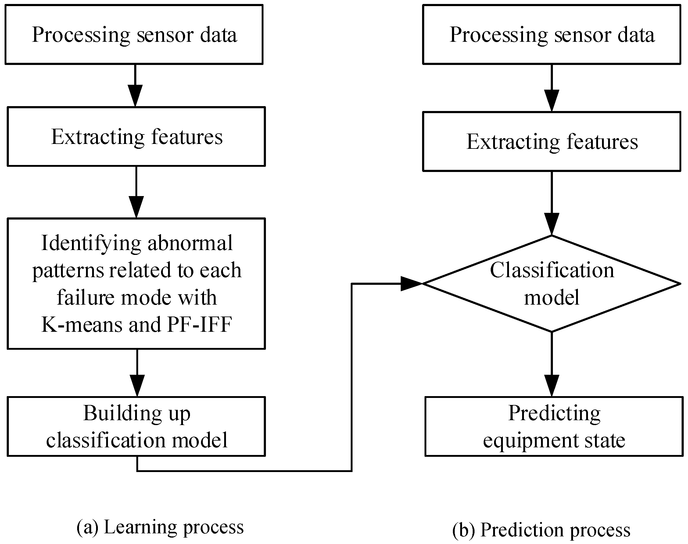
3.1. Learning Process
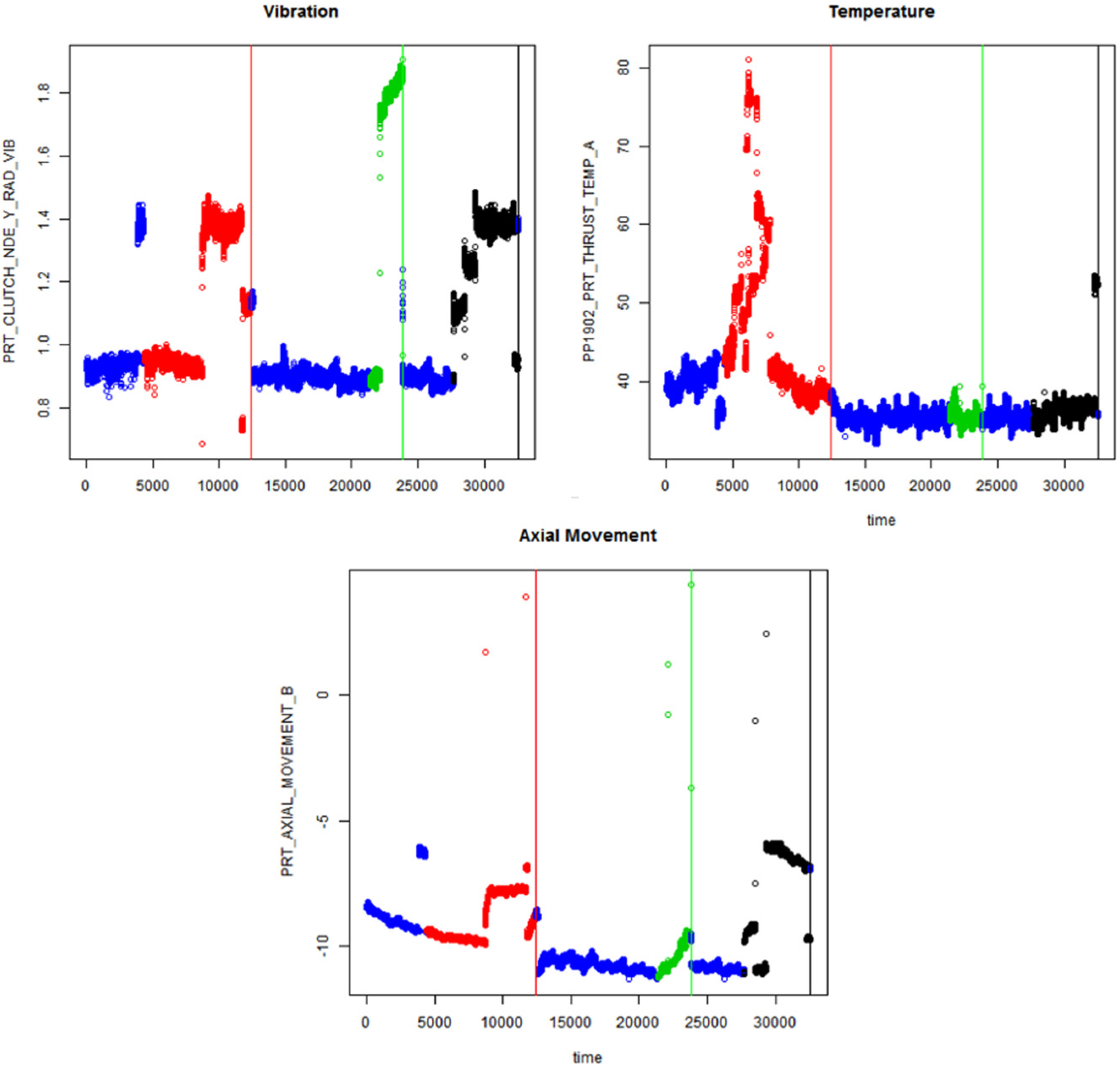
3.1.1. Processing Data
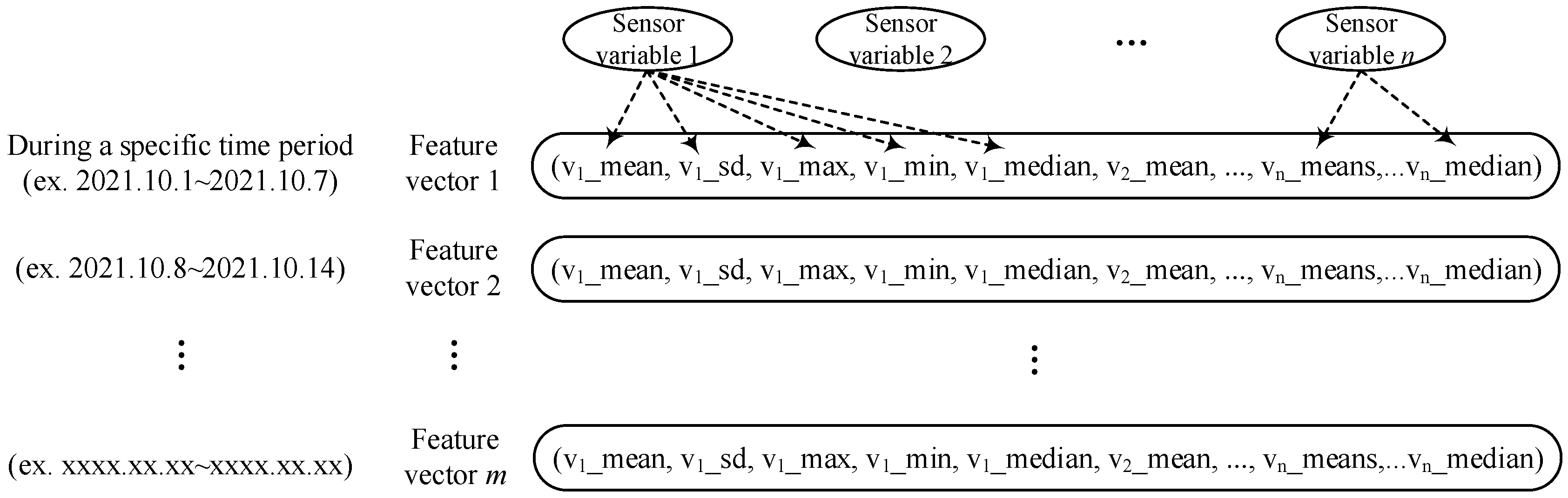
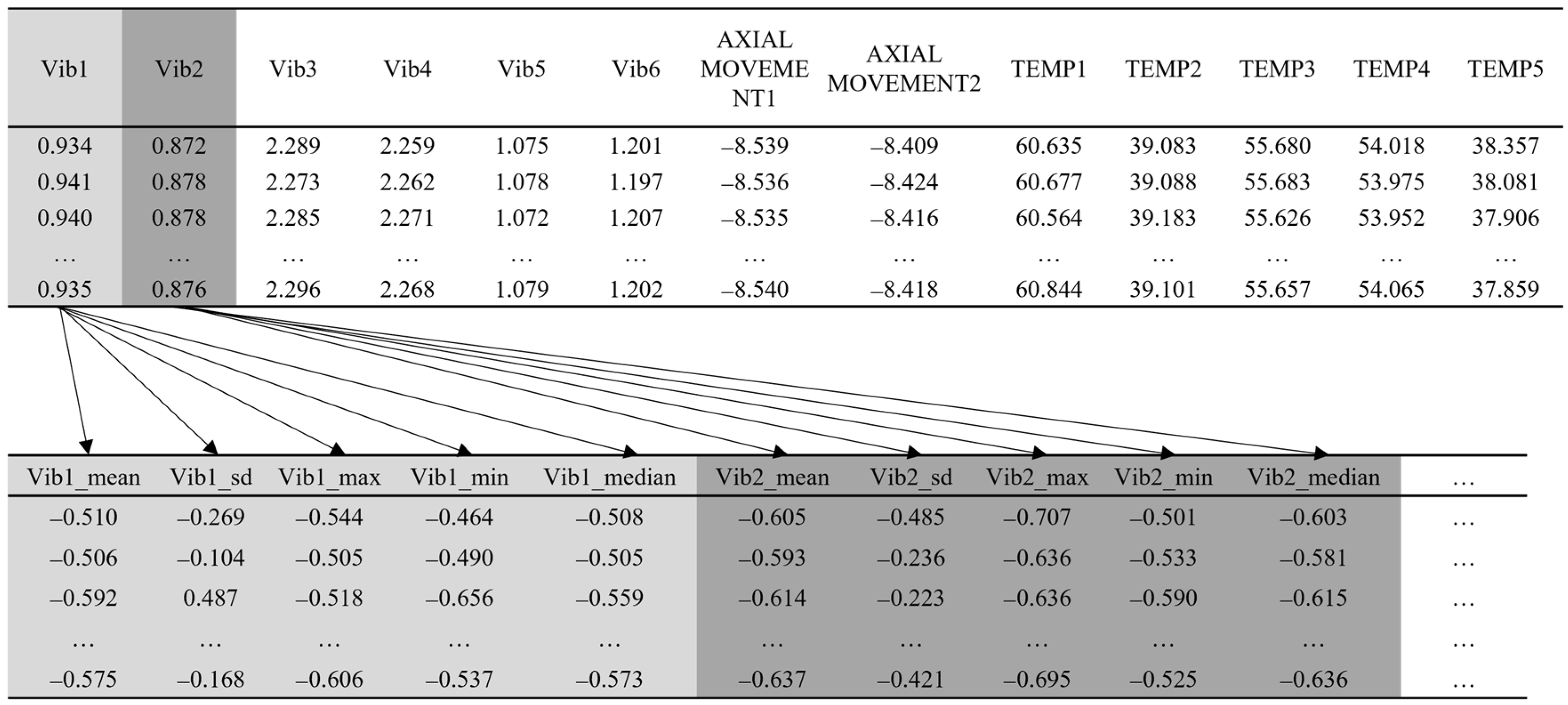
3.1.2. Extracting Feature
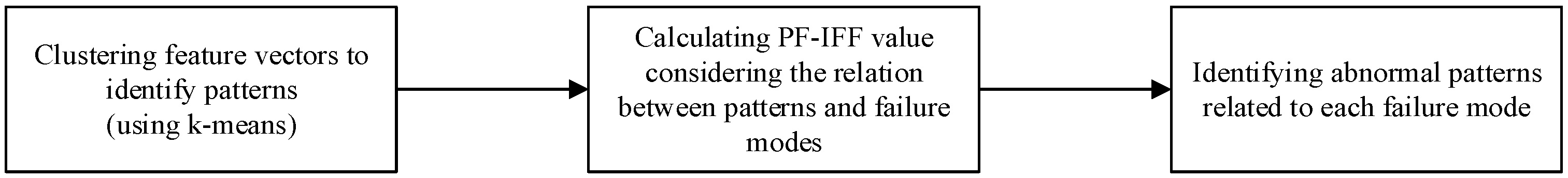
3.1.3. Identifying Abnormal Patterns Related to Each Failure Mode
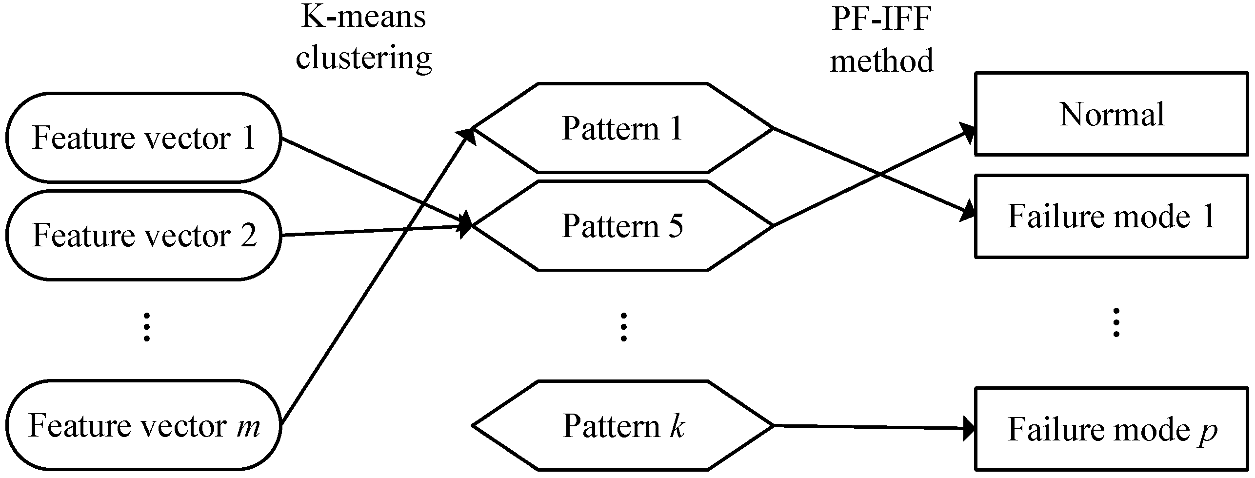
Clustering Feature Vectors to Identify Patterns
Calculating the Relations between Patterns and Failure Modes with PF–IFF
Identifying Abnormal Patterns Related to Each Failure Mode
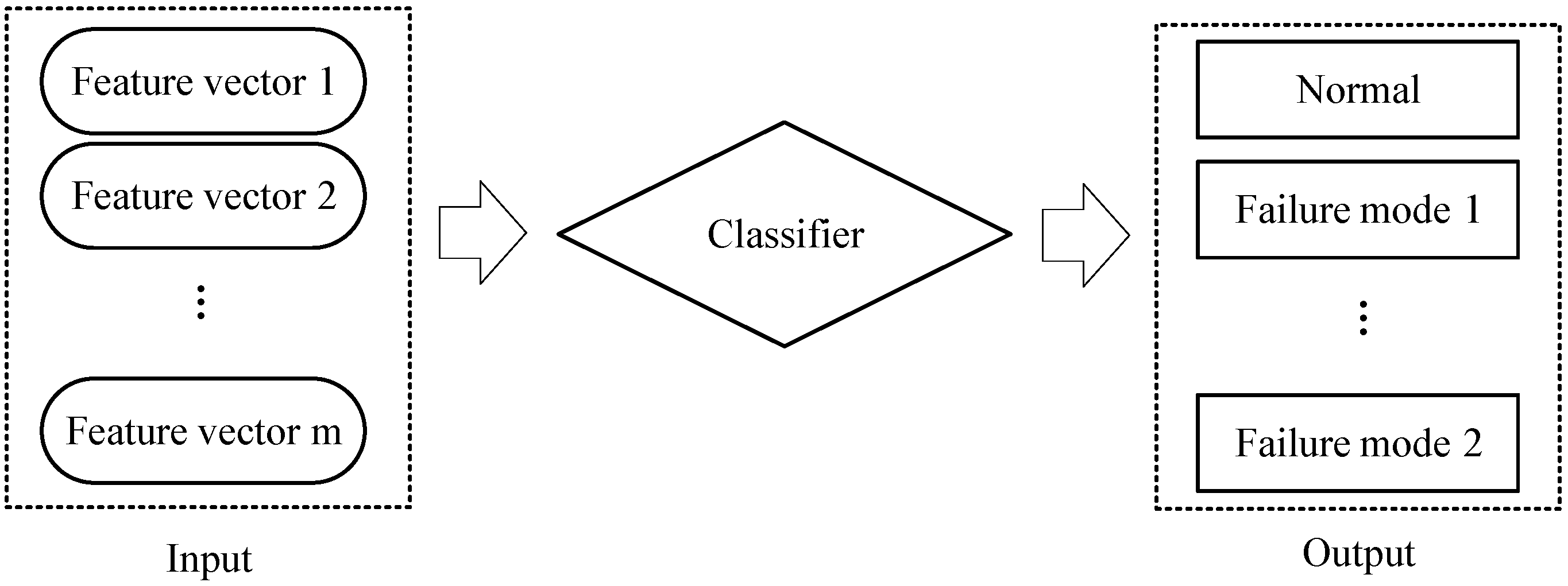
3.1.4. Learning Classification Model
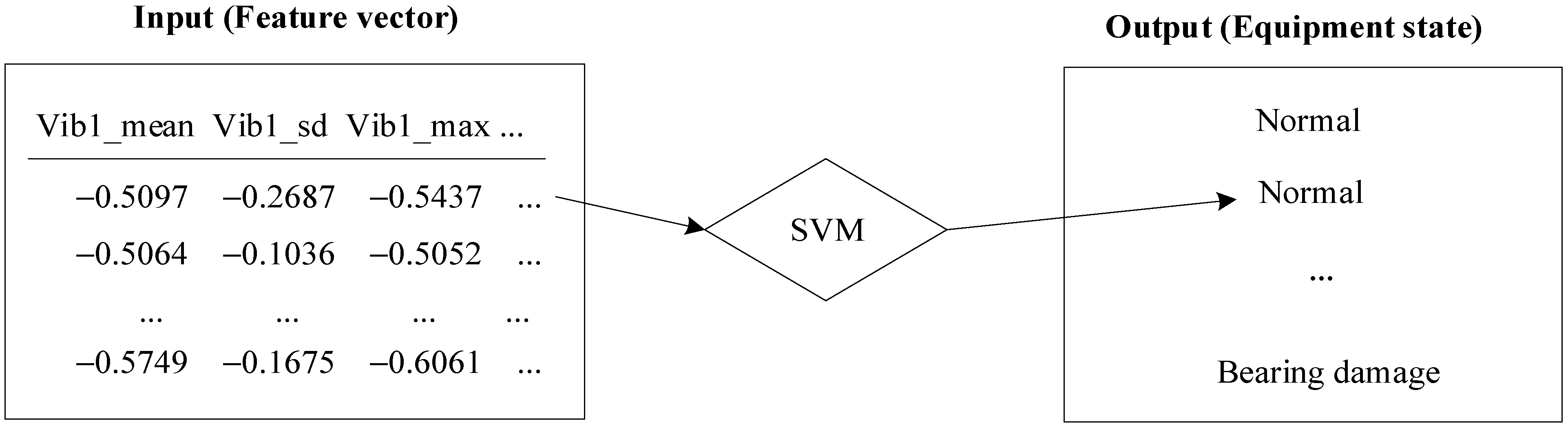
3.2. Prediction Process
4. Case Study
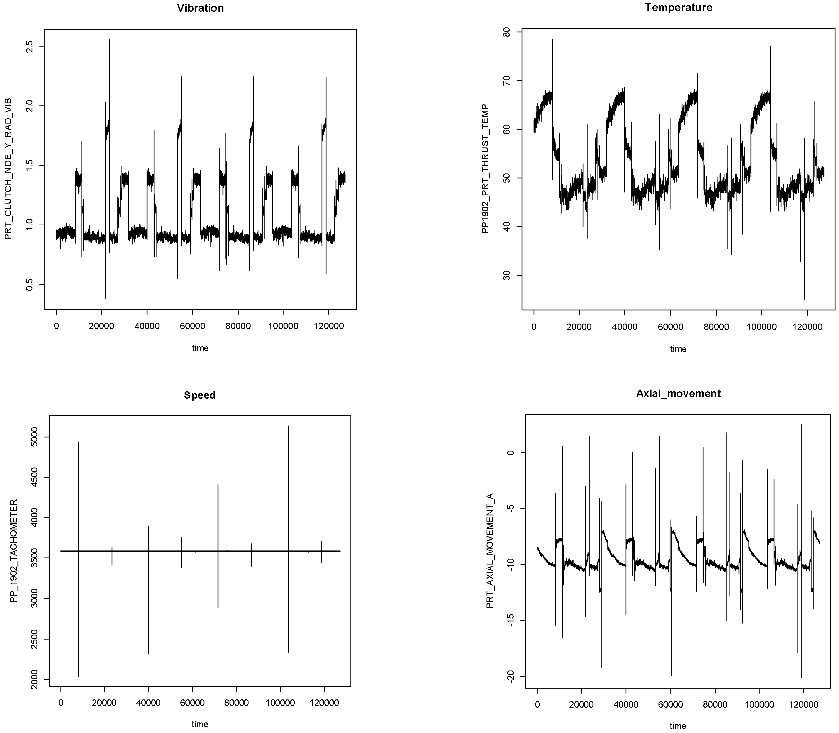
4.1. Processing Data
4.2. Extracting Feature
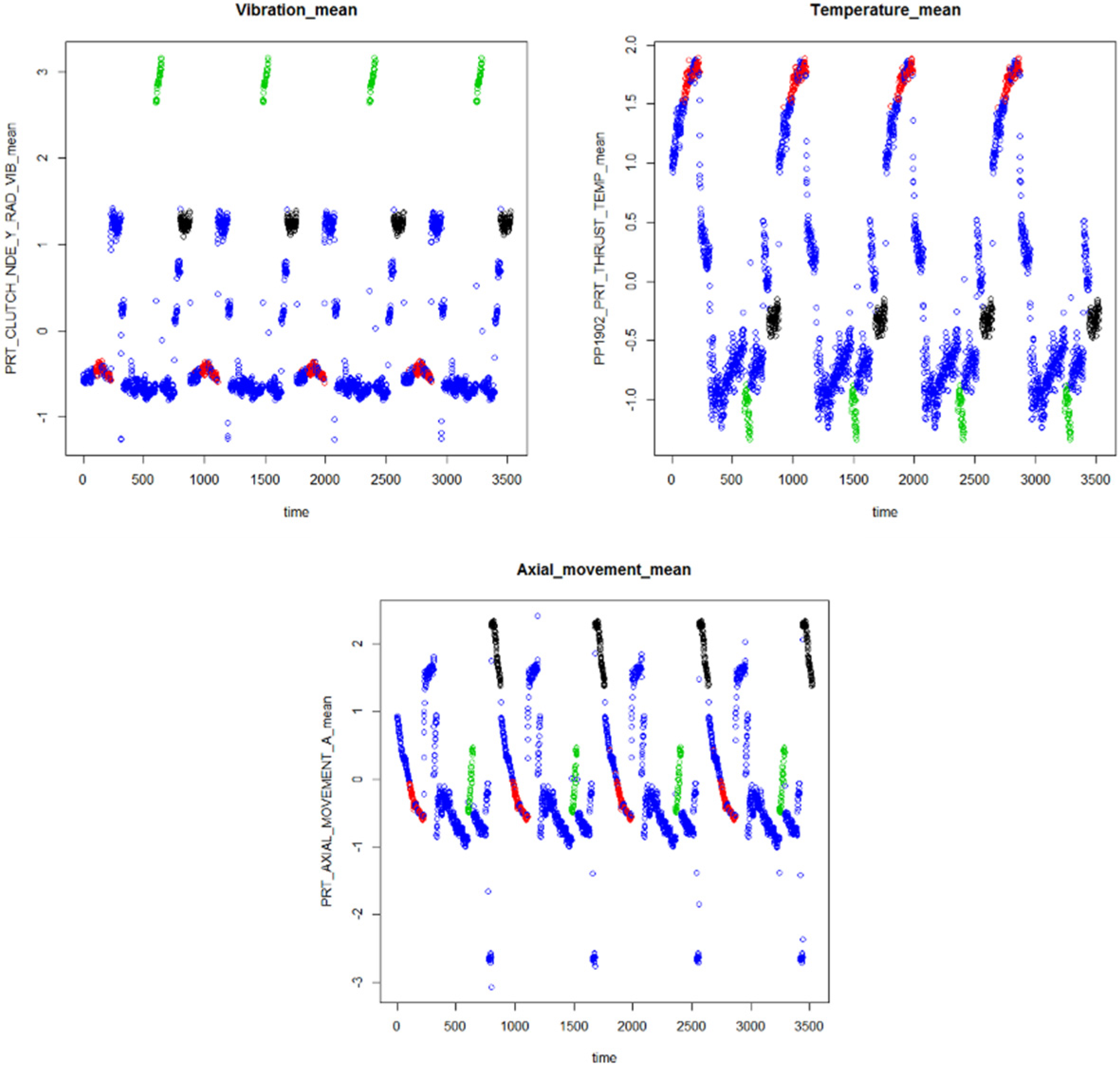
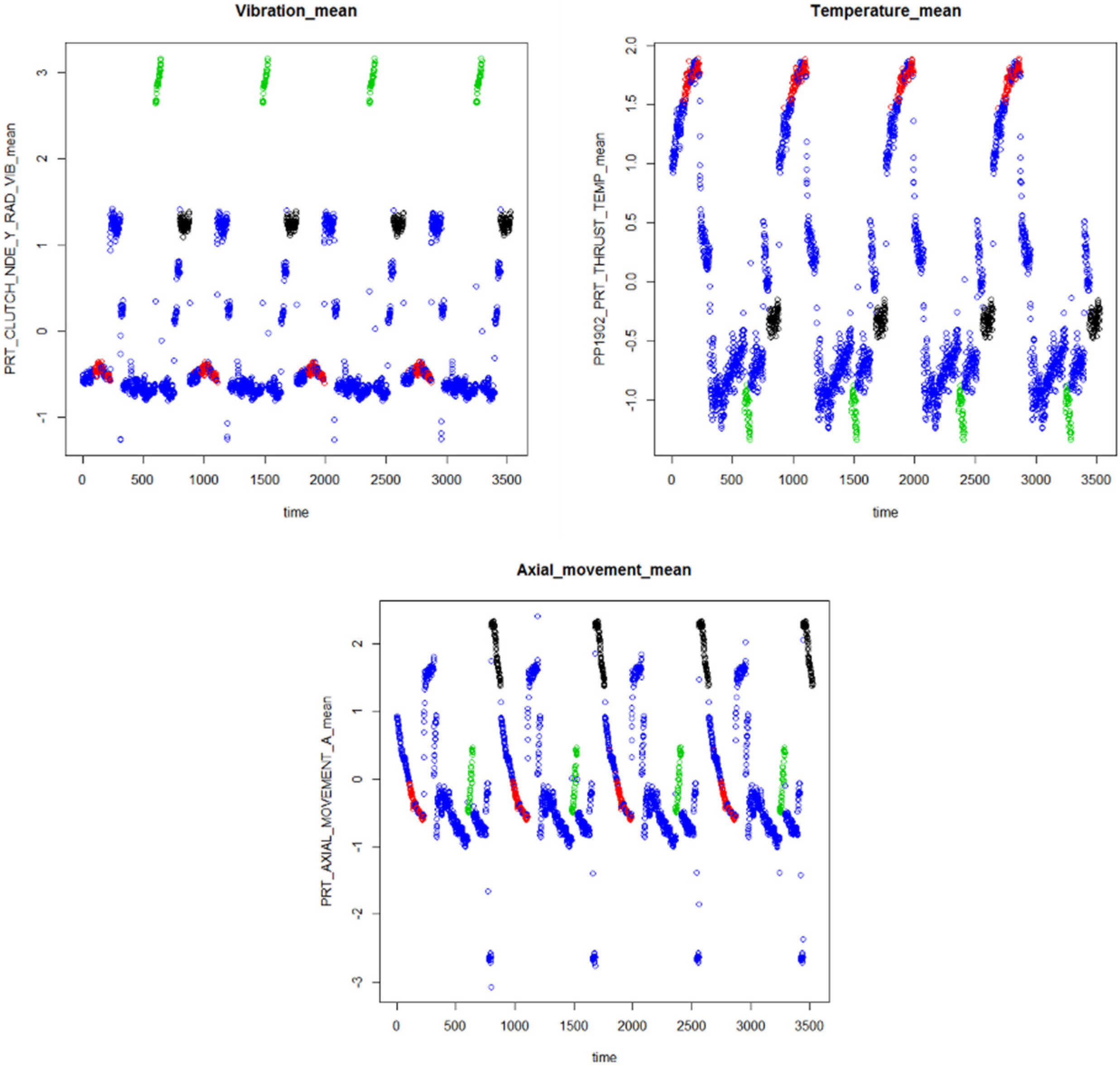
4.3. Identifying Abnormal Patterns Related to Each Failure Mode
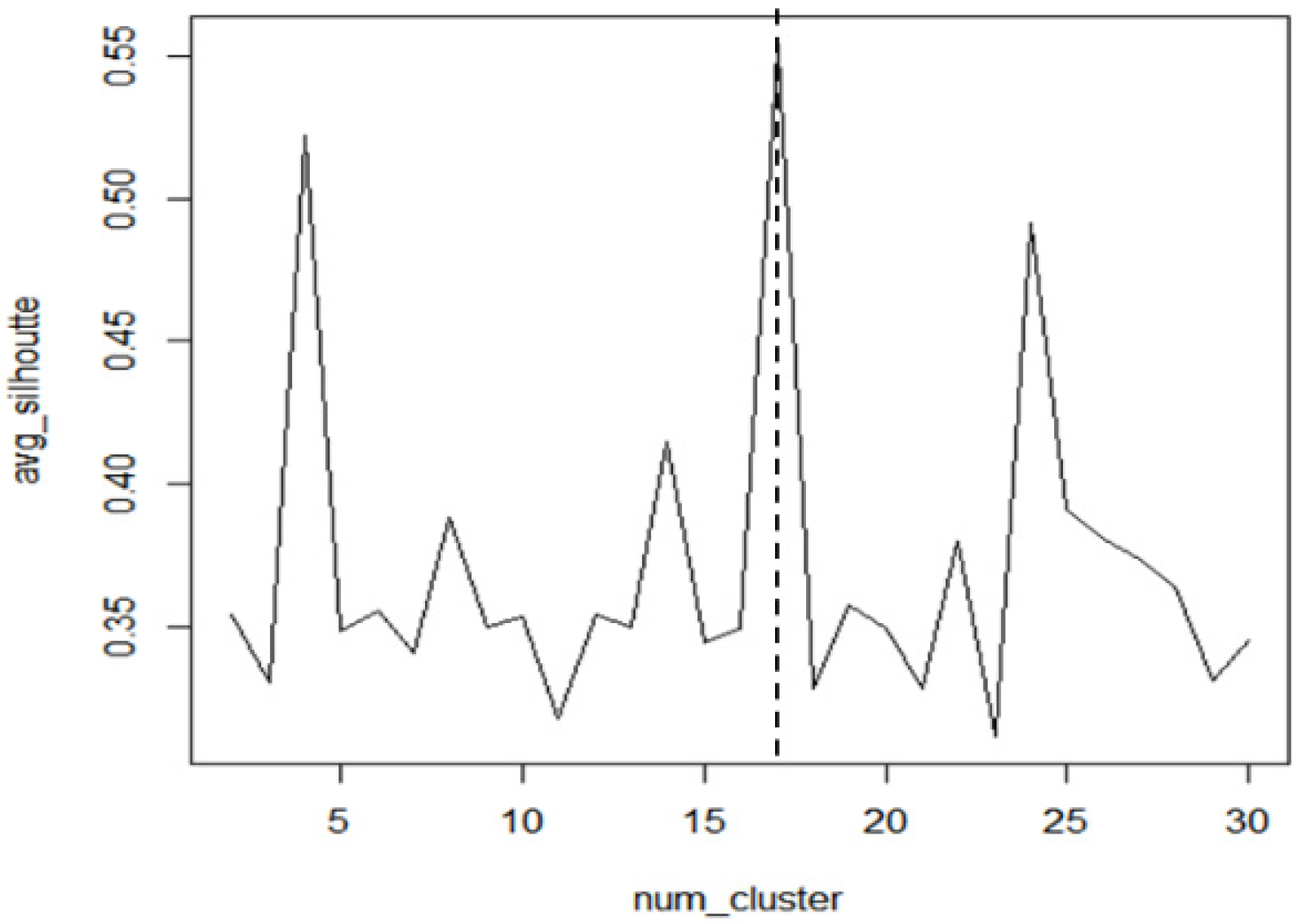
4.3.1. Clustering Feature Vectors to Identify Patterns
4.3.2. Calculating the Relationship between Patterns and Failure Modes
4.3.3. Identifying Abnormal Patterns Related to Each Failure Mode
4.4. Learning Classification Model
4.5. Evaluation
5. Conclusions
Author Contributions
Funding
Data Availability Statement
Conflicts of Interest
Notation
| i | index for feature vector |
| p | index for each pattern |
| f | index for each failure mode |
| F | a set of failure modes |
| k | the number of clusters (patterns) |
| n | the number of variables |
| m | the number of feature vectors |
| FV | a set of feature vectors |
| r | the number of maximum allowable clusters (patterns) |
| average distance between the feature vector i and other points in the same cluster | |
| average distance of the feature vector i for the points in the other clusters | |
| silhouette value in the feature vector i | |
| average silhouette value when the number of clusters is k | |
| the total frequency of pattern p in failure mode f | |
| the frequency of the largest pattern in a certain failure mode | |
| size of failure mode set F (total number of failure modes) | |
| the number of failure modes, including the particular pattern p. |
References
- Arunraj, N.S.; Maiti, J. Risk-based maintenance policy selection using AHP and goal programming. Saf. Sci. 2010, 48, 238–247. [Google Scholar] [CrossRef]
- Shin, J.H.; Jun, H.B. On condition based maintenance policy. J. Comput. Des. Eng. 2015, 2, 119–127. [Google Scholar] [CrossRef] [Green Version]
- Bunks, C.; McCarthy, D.; Al-Ani, T. Condition-based maintenance of machines using hidden Markov models. Mech. Syst. Signal Process. 2000, 14, 597–612. [Google Scholar] [CrossRef]
- Djurdjanovic, D.; Lee, J.; Ni, J. Watchdog Agent—An infotronics-based prognostics approach for product performance degradation assessment and prediction. Adv. Eng. Inform. 2003, 17, 109–125. [Google Scholar] [CrossRef]
- Jardine, A.K.S.; Lin, D.; Banjevic, D. A review on machinery diagnostics and prognostics implementing condition-based maintenance. Mech. Syst. Signal Process. 2006, 20, 1483–1510. [Google Scholar] [CrossRef]
- Salton, G.; Fox, E.A.; Wu, H. Extended Boolean information retrieval. Commun. ACM 1983, 26, 1022–1036. [Google Scholar] [CrossRef]
- Phelan, O.; McCarthy, K.; Smyth, B. Using twitter to recommend real-time topical news. In Proceedings of the Third ACM Conference on Recommender Systems, New York, NY, USA, 23–25 October 2009; pp. 385–388. [Google Scholar]
- Go, G.S.; Jung, W.K.; Shin, Y.G.; Park, S.S.; Jang, D.S. A Study on Development of Patent Information Retrieval Using Text mining. J. Korea Acad.-Ind. Coop. Soc. 2011, 12, 3677–3688. [Google Scholar]
- Trstenjak, B.; Mikac, S.; Donko, D. KNN with TF-IDF based Framework for Text Categorization. Procedia Eng. 2014, 69, 1356–1364. [Google Scholar] [CrossRef] [Green Version]
- Yoo, E.S.; Choi, G.H.; Kim, S.H. Study on Extraction of Keywords Using TF-IDF and Text Structure of Novels. J. Korea Soc. Comput. Inf. 2015, 20, 121–129. [Google Scholar] [CrossRef] [Green Version]
- Dong, M.; He, D. Hidden semi-Markov model-based methodology for multi-sensor equipment health diagnosis and prognosis. Eur. J. Oper. Res. 2007, 178, 858–878. [Google Scholar] [CrossRef]
- Wang, H.Q.; Chen, P. Fault diagnosis of centrifugal pump using symptom parameters in frequency domain. Agric. Eng. Int. CIGR J. 2007, 9, 1–14. [Google Scholar]
- Yang, M.D.; Su, T.C. Automated diagnosis of sewer pipe defects based on machine learning approaches. Expert Syst. Appl. 2008, 35, 1327–1337. [Google Scholar] [CrossRef]
- Fei, S.W.; Zhang, X.B. Fault diagnosis of power transformer based on support vector machine with genetic algorithm. Expert Syst. Appl. 2009, 36, 11352–11357. [Google Scholar] [CrossRef]
- Li, Y.G.; Nilkitsaranont, P. Gas turbine performance prognostic for condition-based maintenance. Appl. Energy 2009, 86, 2152–2161. [Google Scholar] [CrossRef]
- Son, J.H.; Ko, J.M.; Kim, C.O. Feature Based Decision Tree Model for Fault Detection and Classification of Semiconductor Process. IE Interfaces 2009, 22, 126–134. [Google Scholar]
- Zhou, R.; Bao, W.; Li, N.; Huang, X.; Yu, D. Mechanical equipment fault diagnosis based on redundant second generation wavelet packet transform. Digit. Signal Process. 2010, 20, 276–288. [Google Scholar] [CrossRef]
- Wu, B.; Tian, Z.; Chen, M. Condition-based maintenance optimization using neural network-based health condition prediction. Qual. Reliab. Eng. Int. 2013, 29, 1151–1163. [Google Scholar] [CrossRef]
- Muralidharan, V.; Sugumaran, V.; Indira, V. Fault diagnosis of monoblock centrifugal pump using SVM. Eng. Sci. Technol. Int. J. 2014, 17, 152–157. [Google Scholar] [CrossRef] [Green Version]
- Moon, D.S.; Kim, S.H. Development of intelligent fault diagnostic system for mechanical element of wind power generator. J. Korean Inst. Intell. Syst. 2014, 24, 78–83. [Google Scholar]
- Kim, Y.G.; Cho, S.J.; Jun, H.B.; Ha, J.H.; Shin, J.H. A Study on Fault Prediction Method in a Pump Tower of LNG FPSO. Korean J. Comput. Des. Eng. 2016, 21, 111–121. [Google Scholar] [CrossRef]
- Mostafa, S.A.; Mustapha, A.; Hazeem, A.A.; Khaleefah, S.H.; Mohammed, M.A. An agent-based inference engine for efficient and reliable automated car failure diagnosis assistance. IEEE Access 2018, 6, 8322–8331. [Google Scholar] [CrossRef]
- Contreras-Valdes, A.; Amezquita-Sanchez, J.P.; Granados-Lieberman, D.; Valtierra-Rodriguez, M. Predictive data mining techniques for fault diagnosis of electric equipment: A review. Appl. Sci. 2020, 10, 950. [Google Scholar] [CrossRef] [Green Version]
- Abid, A.; Khan, M.T.; Iqbal, J. A review on fault detection and diagnosis techniques: Basics and beyond. Artif. Intell. Rev. 2021, 54, 3639–3664. [Google Scholar] [CrossRef]
- Ng, M.K.; Li, M.J.; Huang, J.Z.; He, Z. On the impact of dissimilarity measure in k-modes clustering algorithm. IEEE Trans. Pattern Anal. Mach. Intell. 2007, 29, 503–507. [Google Scholar] [CrossRef]
- Hartigan, J.A.; Wong, M.A. Algorithm AS 136: A k-means clustering algorithm. J. R. Stat. Soc. 1979, 28, 100–108. [Google Scholar] [CrossRef]
- Rousseeuw, P.J. Silhouettes: A graphical aid to the interpretation and validation of cluster analysis. J. Comput. Appl. Math. 1987, 20, 53–65. [Google Scholar] [CrossRef] [Green Version]
- Jeoung, R.H.; Lee, B.K. Fault Detection Signal for Mechanical Seal of Centrifugal Pump. J. Korean Soc. Saf. 2012, 27, 20–27. [Google Scholar]
- Jeoung, R.H.; Chai, J.B.; Lee, B.H.; Lee, D.H.; Lee, B.K. Feature parameter analysis for rotor fault diagnosis. KSFM J. Fluid Mach. 2012, 15, 31–38. [Google Scholar] [CrossRef]
- Tinga, T. Mechanism Based Failure Analysis; Netherlands Defense Academy Publisher: Den Helder, The Netherlands, 2012. [Google Scholar]
- Cortes, C.; Vapnik, V. Support-vector networks. Mach. Learn. 1995, 20, 273–297. [Google Scholar] [CrossRef]


| Authors | Subject | Approach |
|---|---|---|
| Bunks et al. (2000) [3] | They introduced a CBM method using the Hidden Markov Model (HMM) and carried out case studies based on the data collected from the Westland helicopter gearbox. | Hidden Markov Model |
| Djurdjanovic et al. (2003) [4] | Using sensors to collect multiple attributes and wireless internet technology, they proposed the Watchdog Agent concept to carry out CBM on mechanical devices. | Wavelet Transform, Fourier Transform, Autoregressive Moving Average, etc. |
| Jardine et al. (2006) [5] | They reviewed the CBM research works related to failure diagnostics and prognostics of mechanical systems, mainly focusing on models, algorithms, and techniques for data processing and maintenance decision-making. | CBM review study |
| Shin and Jun (2015) [2] | They introduced CBM definitions, related international standards, CBM procedures, and detailed techniques that were dealt with in previous CBM studies, and also introduced related case studies. | CBM review study |
| Authors | Subject | Approach |
|---|---|---|
| Phelan et al. (2009) [7] | They proposed a method for recommending news articles using real-time Twitter data. When ranking news, they used the TF–IDF technique. | TF–IDF |
| Go et al. (2011) [8] | They proposed a method that enables content-based retrieval using text mining by improving the existing keywords and search expressions in the field of patent searches. In their approach, they used the TF–IDF technique to extract keywords from documents. | TF–IDF |
| Trstenjak et al. (2014) [9] | Based on the KNN algorithm and TF–IDF technique, they suggested a document classification framework. | k-nearest neighbor algorithm, TF–IDF |
| Yoo et al. (2015) [10] | Using the TF–IDF technique and external structure of a novel, they proposed a method of extracting subject words of the novel. | TF–IDF |
| Authors | Subject | Approach |
|---|---|---|
| Dong and He (2007) [11] | Unlike HMMs with fixed state transition probability, the HSMM technique considers the change of the state transition probability over time, suggesting a method to diagnose and predict the condition of equipment. | Hidden semi-Markov model |
| Wang and Chen (2007) [12] | They applied a partly-linearized neural network in order to diagnose the centrifugal pump failure. To this end, they extracted relevant features using a continuous wavelet transform technique. | Continuous Wavelet Transform, Partially-linearized neural network |
| Yang and Su (2008) [13] | They proposed a methodology to diagnose faults in sewer pipes by extracting organizational characteristics of pipe faults in CCTV images using SVM. | SVM, Radial Basis Network, Back-Propagation Neural network |
| Fei and Zhang (2009) [14] | They applied the SVM with the Genetic Algorithm (SVMG) method for diagnosing power transformation failures based on gas information gathered from the equipment. | Support Vector Machine with Genetic Algorithm |
| Li and Nilkitsaranont (2009) [15] | With the model combining linear regression with quadratic regression, they predicted the deterioration of a gas turbine engine. | Regression |
| Son et al. (2009) [16] | They proposed the FDS (Fault Detection System) using a feature-based decision tree based on the data collected from the sensor of the equipment. | Decision Tree |
| Wu et al. (2013) [18] | With the estimator of the remaining life prediction error using an artificial neural network, they develop a method estimating the failure rate threshold corresponding to the lowest maintenance cost. | Artificial Neural Network |
| Muralidharan et al. (2014) [19] | They performed a study to extract features from a centrifugal pump using a continuous wavelet transform technique and to determine equipment failures with SVM for diagnosing equipment failures with vibration data. | Continuous Wavelet Transform, SVM |
| Moon and Kim (2014) [20] | They proposed a diagnostic system using artificial neural networks and wavelet transformations to efficiently diagnose mechanical failures such as mass imbalance and misalignment of axes that occur frequently in wind power generation systems. | Artificial Neural Network, Wavelet Transform |
| Kim et al. (2016) [21] | Using the marine environmental data, they suggested a method for estimating the remaining life of a pump tower, the main structure of LNG FPSO. | K-means clustering, Autoregressive Integrated Moving Average |
| Mostafa et al. (2018) [22] | They proposed an agent-based inference engine and a multi-agent system collaborative module for car failure diagnosis. | Agent-based inference engine based on a forward chaining algorithm |
| Contreras-Valdes et al. (2020) [23] | They reviewed predictive data mining methods for fault detection and diagnosis in electrical equipment. | Review study |
| Abid et al. (2021) [24] | They reviewed the research works related to Fault Detection and Diagnosis (FDD) methods. | Review study |
| Pattern | Bearing Damage | Leakage | Misalignment |
|---|---|---|---|
| 1 | 0.532 * | 0.458 | 0.793 |
| 2 | 0.494 | 0.458 | 0.54 |
| 3 | 0.693 | 1.232 | 0.693 |
| 4 | 0.49 | 0.458 | 0.546 |
| 5 | 0.464 | 0.458 | 0.916 |
| 6 | 0.567 | 0.458 | 0.848 |
| 7 | 0.365 | 0.362 | 0.358 |
| 8 | 0.458 | 0.542 | 0.472 |
| 9 | 0.883 | 0.693 | 0.693 |
| 10 | 0.693 | 1.297 | 0.693 |
| 11 | 0.693 | 0.904 | 0.693 |
| 12 | 1.386 | 0.693 | 0.693 |
| 13 | 0.462 | 0.916 | 0.458 |
| 14 | 0.693 | 0.693 | 1.238 |
| 15 | 0.695 | 0.458 | 0.901 |
| 16 | 0.561 | 0.458 | 0.752 |
| 17 | 0.881 | 0.693 | 0.693 |
| Criterion for State Assignment | Normal | Bearing Damage | Leakage | Misalignment |
|---|---|---|---|---|
| Day 1 | 0.722 * | 0.593 | 0.739 | 0.689 |
| Day 2 | 0.544 | 0.521 | 0.563 | 0.398 |
| Day 3 | 0.500 | 0.466 | 0.548 | 0.499 |
| Day 4 | 0.573 | 0.511 | 0.744 | 0.615 |
| Combination of the Number of Patterns for Each Failure Mode | Normal | Bearing Damage | Leakage | Misalignment |
|---|---|---|---|---|
| BearingDamage:1, Leakage:1, Misalignment:1 | 0.788 * | 0.895 | 0.544 | 0.793 |
| BearingDamage:1, Leakage:1, Misalignment:2 | 0.679 | 0.86 | 0.541 | 0.813 |
| BearingDamage:1, Leakage:1, Misalignment:3 | 0.624 | 0.863 | 0.477 | 0.892 |
| BearingDamage:1, Leakage:2, Misalignment:1 | 0.932 | 0.880 | 0.914 | 0.758 |
| BearingDamage:1, Leakage:2, Misalignment:2 | 0.837 | 0.879 | 0.901 | 0.789 |
| BearingDamage:1, Leakage:2, Misalignment:3 | 0.791 | 0.892 | 0.879 | 0.889 |
| BearingDamage:1, Leakage:3, Misalignment:1 | 0.744 | 0.920 | 0.806 | 0.737 |
| BearingDamage:1, Leakage:3, Misalignment:2 | 0.656 | 0.912 | 0.791 | 0.771 |
| BearingDamage:1, Leakage:3, Misalignment:3 | 0.605 | 0.946 | 0.779 | 0.887 |
| BearingDamage:2, Leakage:1, Misalignment:1 | 0.783 | 0.944 | 0.542 | 0.791 |
| BearingDamage:2, Leakage:1, Misalignment:2 | 0.699 | 0.929 | 0.537 | 0.807 |
| BearingDamage:2, Leakage:1, Misalignment:3 | 0.659 | 0.943 | 0.482 | 0.891 |
| BearingDamage:2, Leakage:2, Misalignment:1 | 0.950 | 0.940 | 0.909 | 0.757 |
| BearingDamage:2, Leakage:2, Misalignment:2 | 0.861 | 0.929 | 0.899 | 0.785 |
| BearingDamage:2, Leakage:2, Misalignment:3 | 0.827 | 0.968 | 0.887 | 0.889 |
| BearingDamage:2, Leakage:3, Misalignment:1 | 0.754 | 0.949 | 0.802 | 0.731 |
| BearingDamage:2, Leakage:3, Misalignment:2 | 0.678 | 0.946 | 0.791 | 0.768 |
| BearingDamage:2, Leakage:3, Misalignment:3 | 0.635 | 0.979 | 0.783 | 0.889 |
| BearingDamage:3, Leakage:1, Misalignment:1 | 0.832 | 0.976 | 0.584 | 0.798 |
| BearingDamage:3, Leakage:1, Misalignment:2 | 0.755 | 0.979 | 0.547 | 0.805 |
| BearingDamage:3, Leakage:1, Misalignment:3 | 0.714 | 0.982 | 0.463 | 0.891 |
| BearingDamage:3, Leakage:2, Misalignment:1 | 0.957 | 0.977 | 0.930 | 0.765 |
| BearingDamage:3, Leakage:2, Misalignment:2 | 0.888 | 0.976 | 0.909 | 0.787 |
| BearingDamage:3, Leakage:2, Misalignment:3 | 0.860 | 0.981 | 0.891 | 0.888 |
| BearingDamage:3, Leakage:3, Misalignment:1 | 0.754 | 0.963 | 0.813 | 0.750 |
| BearingDamage:3, Leakage:3, Misalignment:2 | 0.695 | 0.969 | 0.804 | 0.774 |
| BearingDamage:3, Leakage:3, Misalignment:3 | 0.661 | 0.974 | 0.794 | 0.891 |
| Whether PF–IFF Was Used or Not | Normal | Bearing Damage | Leakage | Misalignment |
|---|---|---|---|---|
| Used | 0.957 * | 0.977 | 0.930 | 0.765 |
| Not used | 0.541 | 0.916 | 0.818 | 0.824 |
Publisher’s Note: MDPI stays neutral with regard to jurisdictional claims in published maps and institutional affiliations. |
© 2021 by the authors. Licensee MDPI, Basel, Switzerland. This article is an open access article distributed under the terms and conditions of the Creative Commons Attribution (CC BY) license (https://creativecommons.org/licenses/by/4.0/).
Share and Cite
Seo, M.-Y.; Hwang, S.-Y.; Lee, J.-H.; Kim, J.-G.; Jun, H.-B. A Study on PF–IFF-Based Diagnosis Model of Plant Equipment Failure. Appl. Sci. 2022, 12, 347. https://doi.org/10.3390/app12010347
Seo M-Y, Hwang S-Y, Lee J-H, Kim J-G, Jun H-B. A Study on PF–IFF-Based Diagnosis Model of Plant Equipment Failure. Applied Sciences. 2022; 12(1):347. https://doi.org/10.3390/app12010347
Chicago/Turabian StyleSeo, Min-Young, Se-Yun Hwang, Jang-Hyun Lee, Jae-Gon Kim, and Hong-Bae Jun. 2022. "A Study on PF–IFF-Based Diagnosis Model of Plant Equipment Failure" Applied Sciences 12, no. 1: 347. https://doi.org/10.3390/app12010347
APA StyleSeo, M.-Y., Hwang, S.-Y., Lee, J.-H., Kim, J.-G., & Jun, H.-B. (2022). A Study on PF–IFF-Based Diagnosis Model of Plant Equipment Failure. Applied Sciences, 12(1), 347. https://doi.org/10.3390/app12010347