Research on Prediction Method of Hydraulic Pump Remaining Useful Life Based on KPCA and JITL

Abstract

Hydraulic pumps are commonly used; however, it is difficult to predict their remaining useful life (RUL) effectively. A new method based on kernel principal component analysis (KPCA) and the just in time learning (JITL) method was proposed to solve this problem. First, as the research object, the non-substitute time tac-tail life experiment pressure signals of gear pumps were collected. Following the removal and denoising of the DC component of the pressure signals by the wavelet packet method, multiple characteristic indices were extracted. Subsequently, the KPCA method was used to calculate the weighted fusion of the selected feature indices. Then the state evaluation indices were extracted to characterize the performance degradation of the gear pumps. Finally, an RUL prediction method based on the k-vector nearest neighbor (k-VNN) and JITL methods was proposed. The k-VNN method refers to both the Euclidean distance and angle relationship between two vectors as the basis for modeling. The prediction results verified the feasibility and effectiveness of the proposed method. Compared to the traditional JITL RUL prediction method based on the k-nearest neighbor algorithm, the proposed prediction model of the RUL of a gear pump presents a higher prediction accuracy. The method proposed in this paper is expected to be applied to the RUL prediction and condition monitoring and has broad application prospects and wide applicability.

1. Introduction

With the rapid development of science and technology and the modern manufacturing industry, the structures and functions of mechanical equipment are gradually shifting toward achieving integration, intelligence, refinement, and comprehensiveness. For a mechanical system, a high integration level and high complexity of the structure and function are associated with a high probability of failure. A fault in one of the mechanical components, or even in a tiny part, if not found and repaired in time, may cause the entire system to fail (so that the machine is unable to operate normally) or lead to property damage or even casualties [1].

A gear pump has the advantages of a small volume, lightweight, good technicality, and strong self-suction. It is commonly used in construction engineering, metallurgy, aerospace, automobile manufacturing, shipping, and other fields. As the “heart” of a hydraulic transmission system, the stable operation of a gear pump is an important requirement for its normal operation. Therefore, conducting appropriate monitoring and maintenance and providing warnings of early failures of gear pumps are highly significant [2].

At present, the methods of signal analysis, monitoring, and fault diagnosis of mechanical equipment are becoming increasingly mature, practical, and specialized. The methods of monitoring and fault diagnosis of mechanical equipment that are extensively used worldwide mainly include vibration analysis, sound analysis, oil sample analysis, and temperature monitoring [3]. Among them, fault diagnosis methods based on vibration monitoring and analysis have the following main advantages: (1) Under the condition in which early failure of mechanical equipment is not evident, the collected vibration signals can still be analyzed to determine its position, degree, and cause. For example, Jiang et al. accurately identified the fault degree of rolling bearings based on a deep learning method [3]; (2) there are various methods for analyzing vibration signals, and the analysis results are intuitive and reliable. Sinao et al. proposed a new method for vibration-based techniques to detect, monitor, and prevent pump cavitations [4]; (3) different characteristic parameters of mechanical equipment vibration signals have different sensitivities to different types of faults, and they have practical physical relevance. Gajjar et al. proposed a Tennessee Eastman process fault detection and diagnosis method using sparse principal component analysis [5]. Therefore, in the vibration analysis and fault diagnosis of mechanical equipment, fault diagnosis methods based on vibration monitoring and analysis have attracted increasing attention of researchers. Lei et al. pointed out that machinery intelligent fault diagnosis is a promising tool to deal with mechanical big data. [6]. In 2019, Jiang et al. first proposed a fault identification method for axial piston pump based on voiceprint characteristics, which solved the problem of inconvenient installation of vibration sensors under special conditions [7]. Because of the uniqueness of a hydraulic system, the installation method and location of a vibration sensor affect the signal acquisition. Moreover, a vibration sensor is frequently installed by pasting or using a magnetic base, which is inconvenient in some cases. Pressure is an important parameter of a hydraulic system, and pressure signals can be conveniently collected. The outlet pressure pulsation of a hydraulic pump is mostly related to its vibration. Therefore, this study considers the outlet pressure signals of a pump as the research object.

In the process of collecting the vibration signals of mechanical equipment, there is frequent interference from noise signals. To analyze a vibration signal accurately and yield the correct diagnosis result, it is necessary to alleviate the associated noise and interference. Zhang et al. [8] applied the wavelet packets transform method to the fault diagnosis of rolling bearings and achieved good diagnosis results. Choe et al. [9] defined wavelet packet transform modulus (WPTM) and presented a WPTM-based PQD feature detection method; experiments show that WPTM has advantages in feature detection. Zhu et al. [10] proposed an adaptive extraction method based on extreme-point symmetric mode decomposition; it was applied to the trend term of machinery signal analysis, and good results were obtained. Hu et al. [11] applied ensemble empirical mode decomposition to rolling bearing fault feature extraction. At the same time, many signal decomposition methods have been applied to signal denoising. For example, Jiang et al. [12] applied local mean decomposition method to hydraulic pump fault signals demodulation. Naeem et al. [13] applied weighted singular value decomposition to enhance the detection performance of a vibration sensor.

Because of its good time–frequency localization analysis ability, wavelet analysis based on Fourier analysis is commonly used in signal processing and other fields. Based on an improved wavelet packet transform method, Huang Yuqing et al. [14] proposed the improved denoising method of fractional wavelet packet transformation, which was subsequently used for filtering and reducing noise signals and showed to have good noise reduction effects. Su Xiuhong [15] combined the denoising method of EMD with the wavelet threshold method, which presents a remarkable signal denoising effect. Tang Ying et al. [16] calculated the maximum singular value modulus of impact signals after wavelet transformation to determine their singular values and subsequently suppressed the maximum singular value to eliminate noise. Yi et al. [17] proposed a novel signal adaptive decomposition algorithm processed in TF domain, which provides adequate information about the time-varying instantaneous frequency. Based on the wavelet theory, Zhang Guangtao et al. [18] proposed the method of multi-wavelet analysis and denoising, which solves the correlation problem of multi-wavelet transform coefficients well and has a good denoising effect.

A pressure signal contains a large amount of useful information [19,20]. Accurate extraction of the key information is not only the basis for hydraulic pump fault diagnosis but also for determining the accuracy of the diagnosis results [21]. The main purpose of feature extraction is to extract and filter out the useful information that can accurately characterize the fault characteristics of a hydraulic pump from pressure signals. At present, the extraction methods of mechanical equipment fault characteristic parameters mainly include time, frequency, and time–frequency domain analysis methods, with the last one combining time and frequency domain features [22]. Because time and frequency domain analyses of gear pumps have the advantages of simple form and convenient calculation, the corresponding characteristic parameters are extensively studied and adopted for identifying the operating state of a gear pump [23,24].

If the maintenance personnel who repair a mechanical equipment can timely and accurately determine its remaining useful life (RUL), then a scientific and appropriate maintenance plan can be formulated and the property losses and casualties caused by untimely monitoring and maintenance can also be effectively avoided [25,26]. Therefore, it is essential to predict the RUL of mechanical equipment on time and accurately.

In recent years, with the rapid approach of the artificial intelligence and data “big bang” era, computer and information technologies have been frequently developed and integrated and artificial intelligence and machine learning methods are being constantly innovated and advanced [27]. In the current research on the analysis and prediction of the RUL of mechanical equipment, artificial intelligence has become a prominent topic [6]. Tan Yuanyuan et al. [28] combined collected field data with accelerated life testing data and introduced conversion and environmental difference factors to improve the prediction and evaluation method of RUL. Sim et al. [29] established a set of RUL prediction and evaluation models for gears and bearings. Kong Guojie et al. [30] established an RUL prediction and evaluation model for artillery barrels and verified its accuracy with a large amount of actual data.

Just in time learning (JITL), a commonly used nonlinear modeling method [31], is also known as lazy learning [32] and locally weighted learning [33]. It uses process data to build local models to achieve high prediction accuracy. Therefore, the JITL modeling method can effectively solve the modeling problems of strongly nonlinear and time-varying industrial processes, and it has been extensively used in the industry [34]. Wang Li et al. [35] first grouped variables by principal component analysis (PCA), subsequently selected similar sample data for each group of variables using the JITL method, and finally predicted the output by Gaussian process regression. The simulation and experimental results showed that the proposed method has good prediction performance. Qi Cheng et al. [36] proposed a JITL method based on second-order similarity, and simulations and experiments verified that it can improve the prediction accuracy of a model. Jin et al. [37] proposed an integrated soft-sensing modeling framework for JITL based on an evolutionary multi-objective optimization method. The experimental results showed the effectiveness and excellence of this method. Guo et al. [38] proposed a JITL framework based on a variational adaptive encoder to solve the problem of non-consideration of the variable uncertainty in industrial processes, and showed the effectiveness of the method based on experiments.

Although the JITL method is commonly recognized, its utilization for predicting the RUL of mechanical equipment is rarely reported. Therefore, this study proposes a prediction method based on JITL to predict the RUL of mechanical equipment on time and accurately.

The evolution processes of many equipment faults follow a certain change rule. To detect faults on time, appropriate methods can be adopted to monitor the operating state of a mechanical equipment and observe the real-time changes in the equipment state [39].

The performance of a mechanical equipment tends to decline during operation, and the performance degradation process is frequently irreversible. The performance degradation of mechanical equipment makes their continuous operation impossible. Timely early warning of machinery equipment failure can be provided using appropriate monitoring methods to monitor the working state of machinery and equipment in real time. This will not only help equipment users to establish an appropriate maintenance and repair plan to prevent unexpected shutdowns of the mechanical equipment during use but also effectively prolong its normal operation time and avoid the economic losses caused by unexpected equipment failures.

The most major feature of data-driven prediction is that it does not require establishing a complex mathematical model for the prediction and evaluation of mechanical equipment. It only needs collection of a large amount of data generated in the industrial field, based on which a model is built. The establishment of a data-driven model can utilize the real-time measurement data sampled by sensors; therefore, the characteristic parameters of the prediction model can be modified on time to accurately reflect the changes in the measured data. Data-driven prediction models mainly include the time-series prediction method [40], artificial neural networks [41], and support vector regression [42]. In this study, the established data-driven prediction model mainly predicts the RUL of a gear pump from two aspects: determining the performance degradation index and constructing an RUL prediction model of a gear pump.

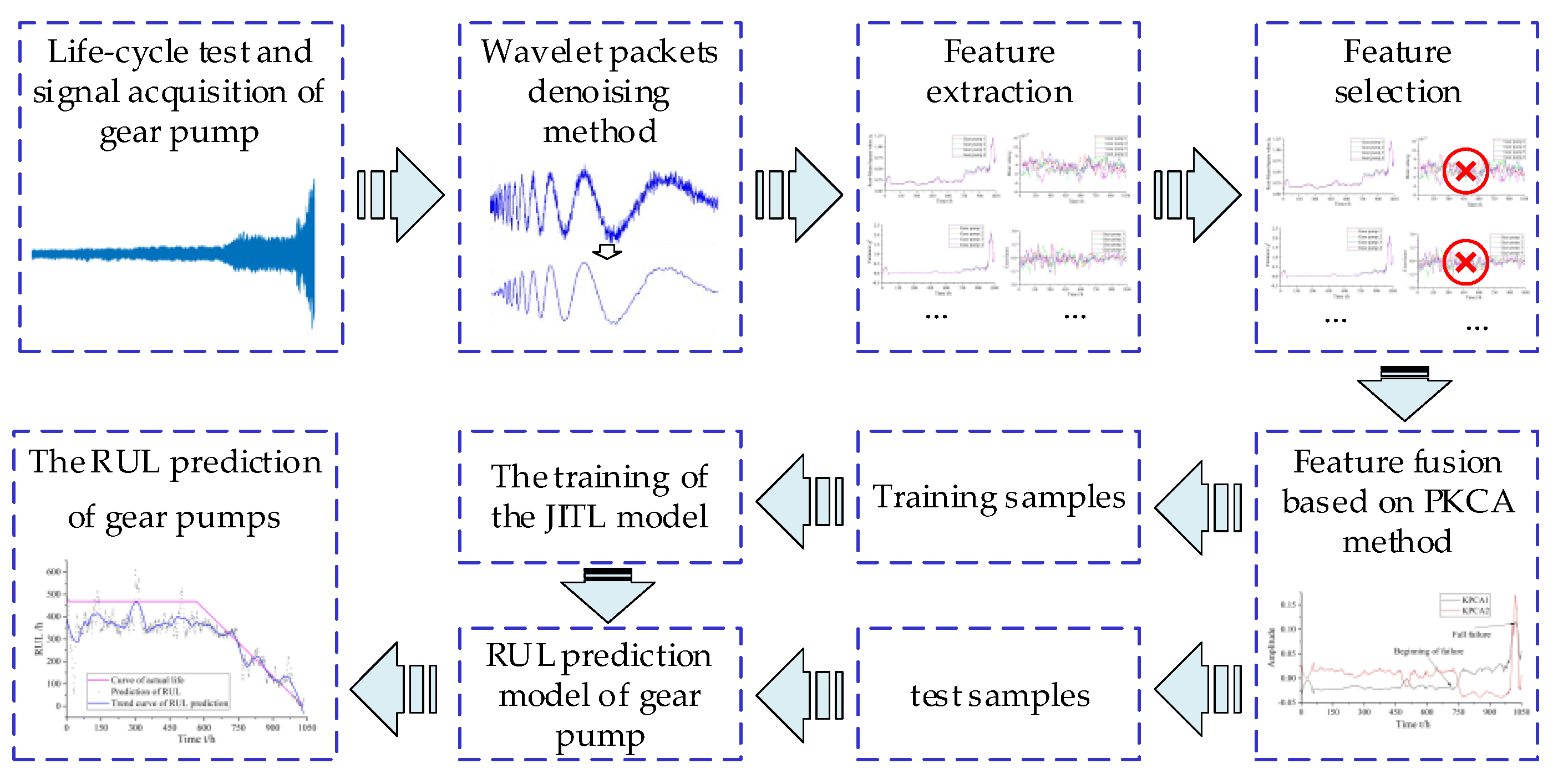
The main research steps of this study are shown in Figure 1. First, the gear pump pressure signals at a pressure port were collected by a pressure sensor. After eliminating the DC component of the collected pressure signals, the wavelet packet denoising method was used to denoise the signals. After denoising, the time- and frequency-domain characteristic indices of the signals were extracted and preliminarily screened. Subsequently, the kernel PCA (KPCA) was used to analyze the screened time- and frequency-domain characteristic indices. The first and second principal components were extracted to identify the performance degradation index of a gear pump. Finally, based on the degradation index, a prediction model based on the k-vector nearest neighbor (k-VNN) JITL method was established for the RUL prediction of a gear pump. The method proposed in this paper was compared to the traditional JITL method based on k-nearest neighbor (k-NN). The results show that the proposed RUL prediction model of a gear pump has a higher prediction accuracy than the traditional method.

2. Wavelet Packet Denoising Method and KPCA Method

In actual field applications or industrial production, when a gear pump fails, the pressure pulsation of its oil pressure port changes. Moreover, most of the gear pump fault information is frequently contained in these pressure pulsations and impacts, such as gear pump fault type, fault location, and fault degree. The pressure signals of a gear pump collected by a sensor contain not only the effective state information but also the noise signals; the latter are unrelated to the state information of the gear pump. Therefore, to extract effective characteristic information from sampled original pressure signals, the first step is to denoise them.

2.1. Wavelet Packets Denoising Method

The wavelet packet transform analysis method is a technical improvement of the wavelet transform analysis method. It is a joint signal analysis method based on time and frequency domains. Compared with the signal analysis method of wavelet transform, the wavelet packet transform analysis method can decompose the low- and high-frequency parts of the upper layer simultaneously. Thus, it overcomes the deficiency of the wavelet transform analysis method, which only analyzes the low-frequency part of a signal.

The method of wavelet packet decomposition and denoising can perform orthogonal decomposition of the collected signals in all frequency bands. An orthonormal basis that can reflect the original characteristics of the signals can be obtained by reasonably selecting the optimal wavelet packet basis function and the decomposition layer number. As shown in Figure 2a, after the original signal is decomposed by wavelet decomposition, the low-frequency coefficients will be decomposed again. As shown in Figure 2b, wavelet packet decomposition not only re-decomposes the low-frequency decomposition coefficients after each layer decomposition, but also re-decomposes the high-frequency coefficients. So, the wavelet packet denoising method is more refined and has better localization ability in the frequency domain than the wavelet denoising method.

In multiresolution analysis, $L^2(R)=\underset{j\in Z}{\oplus }{W}_j$ indicates that it is based on different scale factors j. The Hilbert space, $L^2(R)$, is decomposed into the orthogonal sums of all subspaces ${\mathit{W}}_j(j\in Z)$. Following signal filtering, the signals are expanded based on the wavelet packet basis. Specifically, the signal, $f(n)$, to be analyzed is filtered through a low-pass filter H and a high-pass filter G, and thus, a group of low- and high-frequency signals is obtained. Each signal decomposition further decomposes the l-th frequency band of the upper layer, j + 1, into two sub-bands 2l-th and (2l + 1)-th of the lower layer, j.

Wavelet packet decomposition method: ${\left\{d_{j,k}^{2l}\right\}}_{k\in Z}$ and ${\left\{d_{j,k}^{2l+1}\right\}}_{k\in Z}$ are calculated from ${\left\{d_{j+1,k}^l\right\}}_{k\in Z}$, and the wavelet packet decomposition formula is

$$\{\begin{array}{c}{d}_{j,k}^{2l}={\displaystyle \sum _{m\in Z}{\overline{h}}_{m-2k}{d}_{j+1,m}^l}\\ d_{j,k}^{2l+1}={\displaystyle \sum _{m\in Z}{\overline{g}}_{m-2k}{d}_{j+1,m}^l}\end{array},$$

(1)

where ${\left\{h_k\right\}}_{k\in Z}$ denotes the low-pass filter coefficients, ${\left\{g_k\right\}}_{k\in Z}$ denotes the high-pass filter coefficients, and $g_k={(-1)}^k{\overline{h}}_{1-k}$.

Wavelet packet reconstruction method: ${\left\{d_{j+1,k}^l\right\}}_{k\in Z}$ is calculated from ${\left\{d_{j,k}^{2l}\right\}}_{k\in Z}$ and ${\left\{d_{j,k}^{2l+1}\right\}}_{k\in Z}$, and the wavelet packet reconstruction formula is

$$d_{j+1,m}^l={\displaystyle \sum _{k\in Z}\left[h_{m-2k}{d}_{j,k}^{2l}+g_{m-2k}{d}_{j,k}^{2l+1}\right]},$$

(2)

where Daubechies 4 wavelet is selected for wavelet packet decomposition.

The steps of the wavelet packet denoising process are as follows:

(1)

Optimal wavelet packet decomposition basis determination. The optimal wavelet packet decomposition basis is calculated based on the entropy standard.

(2)

Wavelet packet decomposition of the signal. The number of decomposition layers, M, is determined, and the signal, $f(n)$, is decomposed by an M-layer wavelet packet. In this study, the number of decomposition layers, M, is 3.

(3)

Threshold quantization of the wavelet packet decomposition coefficients. An appropriate threshold is selected to quantify each set of wavelet packet decomposition coefficients. In this study, the default threshold is used to denoise the signals.

(4)

Wavelet packet reconstruction. After the threshold quantization processing in Step 3, the wavelet packet decomposition coefficients are reconstructed using the wavelet packet reconstruction method. Subsequently, after denoising, the time-domain signal, $f_{\mathrm{dn}}(n)$, is obtained.

2.2. Determining Performance Degradation Evaluation Index

Owing to the different types and degrees of hydraulic pump faults, the extracted pressure signal characteristic parameters in the time domain are also different. In general, dimensionless indicators are not directly affected by the operating state of a mechanical equipment; they are only determined by its corresponding probability density functions. However, dimensional indicators are directly affected by the operating state of a mechanical equipment. Both dimensional and dimensionless indicators can directly or indirectly reflect the changing trend of gear pump performance degradation during operation. The time-domain characteristic parameter calculation methods of pressure signals are tabulated in

Table 1. Time-domain characteristic parameters.

Characteristic Parameter	Formula	Characteristic Parameter	Formula
Mean value	$\overline{X}=\frac{1}{N}{\displaystyle \sum _{i=1}^N{f}_{\mathrm{dn}}(i)}$	Absolute mean value	$|\overline{X}|=\frac{1}{N}{\displaystyle \sum _{i=1}^N|f_{\mathrm{dn}}(i)|}$
Variance	${\sigma }^2=\frac{1}{N-1}{\displaystyle \sum _{i=1}^N{\left[f_{\mathrm{dn}}(i)-\overline{X}\right]}^2}$	Standard deviation	$\sigma =\sqrt{\frac{1}{N}{\displaystyle \sum _{i=1}^N{\left[f_{\mathrm{dn}}(i)-\overline{X}\right]}^2}}$
Root-mean-square value	$X_{\mathrm{rms}}=\sqrt{\frac{1}{N}{\displaystyle \sum _{i=1}^N{f}_{\mathrm{dn}}{(i)}^2}}$	Shape factor	$S_{\mathrm{f}}=\frac{X_{\mathrm{rms}}}{\left|\overline{X}\right|}$
Kurtosis	$K=\frac{1}{N}{\displaystyle \sum _{i=1}^N{f}_{\mathrm{dn}}{(i)}^4}$	Crest factor	$C_{\mathrm{f}}=\frac{X_{\max }}{X_{\mathrm{rms}}}$
Peak value	$X_{\max }=\max \left[|f_{\mathrm{dn}}(i)|\right]$	Impulse factor	$I_{\mathrm{f}}=\frac{X_{\max }}{\left|\overline{X}\right|}$
Root amplitude	$X_{\mathrm{r}}={\left[\frac{1}{N}{\displaystyle \sum _{i=1}^N\sqrt{|f_{\mathrm{dn}}(i)|}}\right]}^2$	Kurtosis index	$K_{\mathrm{v}}=\frac{K}{X_{\mathrm{rms}}^4}$
Peak-to-peak value	$X_{\mathrm{pp}}=\max \left[f_{\mathrm{dn}}(i)\right]-\min \left[f_{\mathrm{dn}}(i)\right]$	Clearance factor	$C{L}_{\mathrm{f}}=\frac{X_{\max }}{X_{\mathrm{r}}}$

, where $f_{\mathrm{dn}}(n)$ represents the denoised pressure signal obtained after the wavelet packet denoising, where $n=1,2,3,\dots ,N$ and N is the length of the original signal.

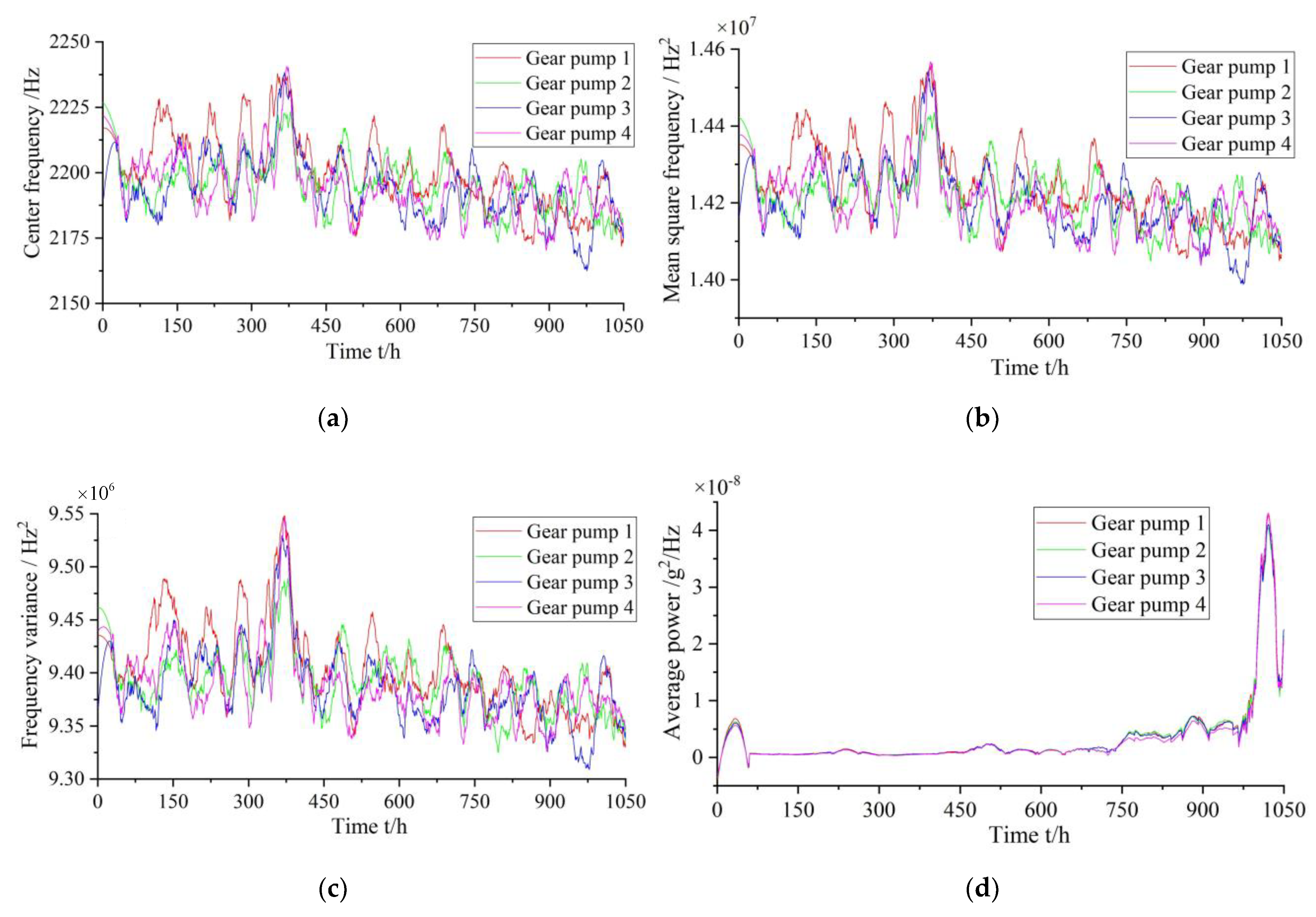
Feature extraction methods based on the time domain are frequently unable to accurately determine the performance degradation trend of mechanical equipment. Therefore, an extraction method based on frequency-domain features is used. First, the power spectral density of the collected mechanical equipment time-domain signals is calculated. Subsequently, the frequency-domain characteristics of the time-domain signals are calculated based on the power spectral density; therefore, the performance degradation trend of the mechanical equipment can be determined more intuitively and accurately. The calculation methods of the characteristic parameters in the relevant frequency domain are summarized in

Table 2. Frequency-domain characteristic parameters.

Characteristic Parameter	Formula	Characteristic Parameter	Formula
Gravity frequency	$CF=\frac{{\displaystyle \sum _{f=0}^{f_{\max }}[f\times S(f)]}}{{\displaystyle \sum _{f=0}^{f_{\max }}S(f)}}$	Frequency variance	$FV=MSF-{(CF)}^2$
Mean square frequency	$MSF=\frac{{\displaystyle \sum _{f=0}^{f_{\max }}[f^2\times S(f)]}}{{\displaystyle \sum _{f=0}^{f_{\max }}S(f)}}$	Average power	$f_1=\frac{{\displaystyle \sum _{f=0}^{f_{\max }}S(f)}}{f_{\max }}$

.

The $f_{\max }$ is the upper limit of the analysis frequency band and $S(f)$ is the amplitude of the power spectrum at frequency $f$.

2.3. KPCA Method

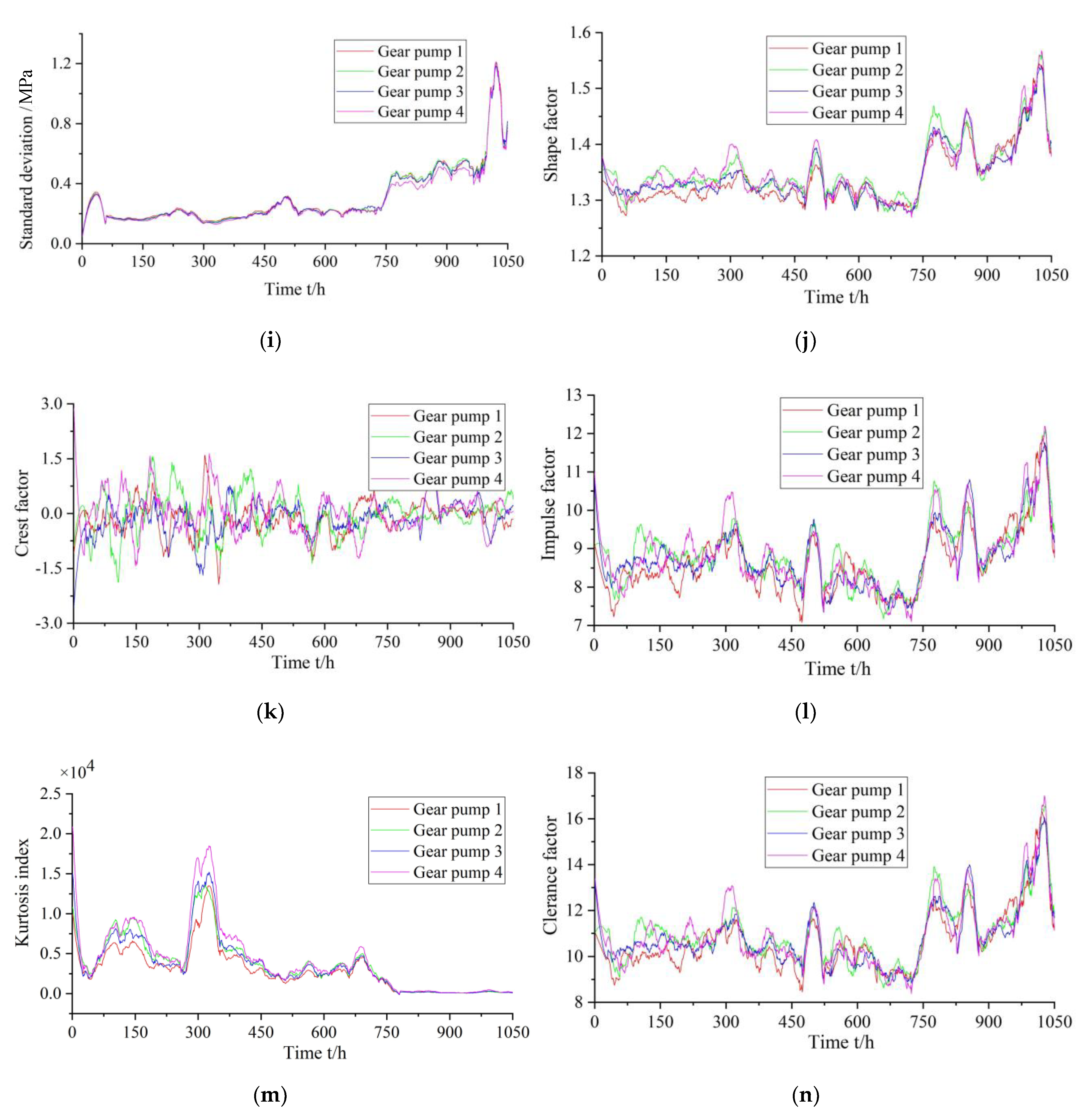
In traditional methods, as a gear pump performance degradation characteristic index, a single time- or frequency domain-characteristic index is frequently used as the basis. Owing to the variability and complexity of the gear pump operation process, a single index cannot accurately and comprehensively represent the faults and performance degradation information during its operation. Therefore, it is necessary to consider and extract multiple appropriate features to achieve comprehensive characterization of a gear pump performance degradation trend. For obtaining the performance degradation characteristic index of a gear pump, in this study, multiple characteristic parameters from the time and frequency domains are selected, including variance, root-mean-square value, peak value, root amplitude, peak-to-peak value, absolute mean value, standard deviation, shape factor, clearance factor, and average power. Subsequently, the dimensionality reduction calculation is performed for the selected multiple characteristic indicators. Finally, the characteristics after the dimensionality reduction are used as the performance degradation evaluation index of the gear pump.

PCA [43] is a traditional mathematical linear transformation analysis method. The basic principle of the PCA method is the linear transformation of the original variables with some correlation into a set of uncorrelated variables, during which process the total variance remains unchanged. The KPCA method extracts the principal components from the original data information by a nonlinear transformation by some technical improvements of the PCA method. First, the input space is transformed into a high-dimensional space by a nonlinear transformation. Subsequently, the principal components in the information are nonlinearly analyzed in the high-dimensional space. The specific method is as follows:

Let the training sample set be $X=\left\{x_i|i=1,2,\dots ,P\right\}$, where $x_i\in R^Q$ is a column vector and $P$ is the number of training samples. The KPCA method nonlinearly maps a $Q$-dimensional original vector from the original input space, $R^Q$, to a high-dimensional space, $F$, represented as $\phi :R^Q\to F$. The sample in $F$ is represented as $\phi (x_i)$, and it satisfies ${\displaystyle {\sum }_{i=1}^P\phi (x_i)}=0$. Therefore, the sample covariance matrix in the $F$ space can be expressed as

$$C=\frac{1}{P}{\displaystyle \sum _{i=1}^P\mathsf{\phi }(x_i)\mathsf{\phi }{(x_i)}^T}.$$

(3)

The eigen decomposition of the covariance matrix, $C$, can be obtained as follows:

$${\lambda }_i{v}_i=\mathit{C}{v}_i,i=1,2,\cdots ,P,$$

(4)

where $v_i$ is the eigenvector corresponding to the eigenvalues, ${\lambda }_i$, in the $F$ space, and all eigenvalues of $C$ are non-negative. Without the loss of generality, $0\le {\lambda }_1\le {\lambda }_2\le \dots \le {\lambda }_P$ are set, and the corresponding eigenvectors, $v_1,v_2,\dots ,v_P$, can be expanded by the sample, $\phi (x_i)$, in the $F$ space as follows:

$$v_r={\displaystyle \sum _{i=1}^P{\alpha }_i^r\mathsf{\phi }(x_i)},$$

(5)

where ${\alpha }_i(i=1,2,\dots ,P)$ are the correlation coefficients.

The inner product of each sample $\phi (x_i)$ with Equation (4) is obtained as follows:

$${\lambda }_r\langle \phi (x_i),v_r\rangle =\langle \phi (x_i),C{v}_r\rangle ,i,r=1,2,\dots ,P.$$

(6)

Based on Equations (5) and (6), the following can be obtained:

$${\lambda }_r{\displaystyle \sum _{i=1}^P{\alpha }_i^r}\langle \phi (x_r),\phi (x_i)\rangle =\frac{1}{P}{\displaystyle \sum _{i=1}^P{\alpha }_i^r}\langle \phi (x_r),{\displaystyle \sum _{q=1}^P\phi (x_q)}\rangle \langle \phi (x_q),\phi (x_i)\rangle ,$$

(7)

where $r,q=1,2,\dots ,P$.

A $P\times P$-dimensional matrix $K$ is defined, where $k_{iq}=\langle \phi (x_i),\phi (x_q)\rangle$ and $i,q=1,2,\dots ,P$. Because $K$ is a symmetric matrix, $k_{iq}=k_{qi}$, Equation (7) can be expressed as

$$P{\lambda }_r{\alpha }^r=K{\alpha }^r,$$

(8)

where $P{\lambda }_r$ is the eigenvalue of $K$ and ${\alpha }^r={[{\alpha }_1^r,{\alpha }_2^r,\dots ,{\alpha }_P^r]}^T$ is the corresponding eigenvector. Let the eigenvectors corresponding to the eigenvalues greater than zero be ${\alpha }^a,{\alpha }^{a+1},\dots ,{\alpha }^P$, respectively. $v_r(r=a,a+1,\dots ,P)$ is normalized to obtain $P{\lambda }_r\langle {\alpha }^r,{\alpha }^r\rangle =1$; therefore, the projection of sample $\phi (x)$ on $v_r$ is

$$t_r(x)=\langle v_r,\phi (x)\rangle ={\displaystyle \sum _{i=1}^P{\alpha }_i^r\langle \phi (x_i),\phi (x)\rangle },$$

(9)

where $t_r(x)$ is the $r$-th nonlinear principal component corresponding to $\phi$. All principal components are combined into vector $t(x)={\left[t_a(x),t_{a+1}(x),\dots ,t_P(x)\right]}^T$ as the sample feature.

To overcome the problem that the high-dimensional $F$ space makes solving $t_r(x)$ difficult, based on the Mercer theorem [44], a kernel function $K_1\left(x_i,x\right)=\langle \phi (x_i),\phi (x)\rangle$ is used to replace the dot product operation of the $F$ space. Therefore,

$$t_r(x)=\langle v_r,\phi (x)\rangle ={\displaystyle \sum _{i=1}^P{\alpha }_i^r{K}_1\left(x_i,x\right)}.$$

(10)

To solve the problem that the sampled data do not satisfy ${\displaystyle {\sum }_{i=1}^P\phi (x_i)}=0$, sample $\phi (x_i)$ in the $F$ space can be replaced by Equation (11).

$$\tilde{\phi }(x_i)=\phi (x_i)-\frac{1}{P}{\displaystyle \sum _{i=1}^P\phi \left(x_i\right)}.$$

(11)

The kernel matrix, $K$, in Equation (8) is replaced by $\overline{K}$.

$$\overline{K}=K-I_{P}K-K{I}_P+I_{P}K{I}_P,$$

(12)

where $I_P$ is a $P\times P$-dimensional identity matrix with coefficient $1/P$.

The radial basis function (RBF) kernel function has many advantages, such as wide convergence range, good positive definiteness of the transformation matrix, few parameters, and simple calculation. In data processing, the accuracy and speed of the RBF kernel function are better than those of other kernel functions. Therefore, the RBF kernel function is selected as the kernel function in the KPCA method as

$$K_1(x,x_i)=\exp [-\frac{{\Vert x-x_i\Vert }^2}{2{\sigma }^2}].$$

(13)

The cumulative percent variances (CPVs) of the principal components are calculated to select the components that meet the conditions. Finally, the number of principal components is determined based on the actual requirements.

The method and process using the CPVs as the basis for selecting the principal components are as follows: First, the corresponding initial data samples are calculated and processed to obtain the covariance matrix. Subsequently, the corresponding eigenvectors are sorted in descending order of the corresponding eigenvalues, and finally, the number of principal components that meets the requirements is selected. The variance contribution rate of a single principal component is

$${\zeta }_r=\frac{{\lambda }_r}{{\displaystyle \sum {}_{r=1}^P{\lambda }_r}}(r=1,2,\dots ,P),$$

(14)

where ${\zeta }_r$ represents the percent variance of the r-th principal component.

The CPV calculation method of the first s principal components is as follows:

$$CPV=\frac{{\displaystyle \sum {}_{r=1}^s}{\lambda }_r}{{\displaystyle \sum {}_{r=1}^P{\lambda }_r}}\times 100\% (s<P),$$

(15)

where P is the total number of eigenvectors.

The CPV size is typically set based on the operating states of the system when using the KPCA method to analyze and calculate the data information. Among the current KPCA methods, CPV is the most extensively used for selecting the number of principal components, and it is relatively easy to implement. In general, to simplify the number of variables in the original sample, reduce the complexity of the data structure, and simultaneously maximize the retention of most useful information in the original sample, the CPV is generally set as at least 85%.

3. Principle of JITL Method

The principle of the JITL method is “similar input data produce similar output data.” Its basic workflow is to store a large amount of sample information in the sample data memory. Based on the actual input data, data similar to the input sample data are found in the sample data storage, and subsequently the corresponding output data of the input data are obtained from the sample data information.

For a nonlinear mapping of multiple inputs and single output, $f:R^n\to R$, it is assumed that the input and output data of the system (i.e., ${\left\{{\mathit{x}}_q,y_q\right\}}_{q=1}^V$, where V is the number of training samples) can be measured. Moreover, the input and output data have the following functional relationship:

$$y_q=f\left(x_q\right)+{\xi }_q,$$

(16)

where $x_q=\left\{x_{i,q}|i=1,2,\dots ,T,q=1,2,\dots ,V\right\}$ represents the input sample data and T is the dimension of the input sample data. The output sample data are $y_q\in R$. ${\xi }_q$ is an independent random variable with a zero mean and a variance of ${\sigma }^2$.

The JITL method establishes a model in a certain space by recursion to predict the output. The input and output relationship of the established model is described as follows:

$$f\left(x_q,\theta \right)=x_q^T\theta ={\theta }_0+x_{1,q}{\theta }_1+x_{2,q}{\theta }_2+\dots +x_{T,q}{\theta }_T,$$

(17)

where $\theta ={\left[{\theta }_0,{\theta }_1,\dots ,{\theta }_T\right]}^T$ represents the sub-model parameters. Combined with a historical database, mapping in the local space is established to obtain the model output value, ${\widehat{y}}_q$. Therefore, the predicted output problem can be solved using an optimal solution, and the formula is as follows:

$$\min {\displaystyle \sum _{(x_q,y_q)\in {\mathbf{\Omega }}_k}{\left[y_q-f(x_q,\theta )\right]}^2{w}_q},$$

(18)

where ${\mathbf{\Omega }}_k$ is the local space consisting of k sample data near $x_q$. $f$ is the mapping relationship between input data $x_q$ and output data $y_q$. $w_q$ is the weight corresponding to the q-th historical sample data, which represents the weight of the influence of the q-th sample data contained in the local sample space on the model output.

The selection of the local space has a significant influence on the accuracy of the sub-models. For the input data, $x_q$, the selected local space is used to select the appropriate historical data. These historical data consist of k samples that are most similar to the input data, $x_q$. To select historical data similar to the input vector, $x_q$, some scholars have proposed k-NN, k-surrounding neighbors, k-bipartite neighbors, and other methods to screen the modeling data. However, these methods mainly refer to the Euclidean distance as the basis for modeling, which is insufficient for fully exploring the internal relationships among the input and nearest data. In [45], the k-VNN method was proposed, which considers both the Euclidean distance and angle relationship between two vectors. Therefore, the k-VNN method is used as the neighborhood selection criterion in this study.

As we all know, k-VNN considers both the Euclidean distance and angle relationship between two vectors, while k-NN mainly refers to the Euclidean distance as the basis for modeling, which is insufficient for fully exploring the internal relationships among the input and nearest data. Therefore, sample selection method based on k-VNN of the RUL prediction method can significantly improve the prediction accuracy of the RUL prediction model.

Assuming that the data in the historical database are $x_i$ and the input data of the model are denoted by $x_q$; the Euclidean distance, $d(x_i,x_q)$; and the two vector angles, $\beta (x_i,x_q)$, between the input data, $x_q$, and the historical data, $x_i$, can be expressed as

$$\{\begin{array}{c}d(x_i,x_q)={\Vert x_i-x_q\Vert }_2\\ \beta (x_i,x_q)={\cos }^{-1}(\frac{x_{\mathrm{i}}^{\mathrm{T}}{x}_q}{{\Vert x_i\Vert }_2\cdot {\Vert x_q\Vert }_2})\end{array},$$

(19)

When constructing the neighborhood, ${\mathbf{\Omega }}_k$, of the input vector, $x_q$, the relationship between the Euclidean distance and the angle of the data information, $x_i$ and $x_q$, are comprehensively considered.

When the angle between $x_i$ and $x_q$ is large (i.e., $\cos \beta (x_i,x_q)<0$), it is considered that the information vector of the sample data deviates from the current input vector, $x_q$, and does not meet the requirements of the local modeling of the system. Therefore, the sample data information should not be used to construct the modeling neighborhood. When the angle between $x_i$ and $x_q$ is small (i.e., $\cos \beta (x_i,x_q)>0$), it is considered that the information vector of the sample data is close to the current input vector, $x_q$, and meets the requirements of the local modeling of the system. Therefore, the sample data information is used to construct the modeling neighborhood.

The neighborhood selection criterion, $D(x_i,x_q)$, of input vector  is constructed as follows:

$$D(x_i,x_q)=\gamma \cdot e^{-d(x_i,x_q)}+(1-\gamma )\cdot \cos \beta (x_i,x_q),$$

(20)

where $\gamma$ is the weight factor and $\gamma \in [0,1]$. Because $d(x_i,x_q)\ge 0$ and $\cos \beta (x_i,x_q)\in [0,1]$, $D(x_i,x_q)\in [0,1]$.

Equation (20) indicates that $D(x_i,x_q)$ considers not only the Euclidean distance of the vectors but also the angle information between the vectors. Considering the Euclidean distance and the angle information, the similarity between vectors $x_i$ and $x_q$ can be more comprehensively reflected. Two similar vectors imply large neighborhood selection criteria $D(x_i,x_q)$. This indicates that the historical data, $x_i$, have a significant influence on the sub-model (i.e., the weight coefficient, $w_q$, is large). Therefore, the following is set:

$$D(x_i,x_q)=w_q,$$

(21)

that is,

$$\min {\displaystyle \sum _{(x_i,y_i)\in {\mathbf{\Omega }}_k}{\left[y_i-f(x_i,\theta )\right]}^{2}D(x_i,x_q)}.$$

(22)

It is considered that in the neighborhood of the input vector, $x_q$, the local model of the system can be represented by a linear polynomial. First, it is necessary to provide the range size of the neighborhood, k, of the current input vector, $x_q$; $[k_m,k_M]$ indicates that the number of vectors required for the local modeling of the current input vector, $x_q$, is at least $k_m$ and at most $k_M$. $D(x_i,x_q)$ is taken as a criterion for selecting samples, and the current input vector, $x_q$, is used to construct their neighborhood, ${\mathbf{\Omega }}_k$. Because a large $D(x_i,x_q)$ implies high similarity degree between the vectors, the descending order arrangement method is adopted to construct the neighborhood as follows:

$${\mathbf{\Omega }}_k=\{(x_1,y_1),(x_2,y_2),\dots ,(x_k,y_k)|D_1>D_2>\dots >D_k\}.$$

(23)

Therefore, the problem of solving Equation (18) is transformed into an optimal selection problem of neighborhood k. To improve the prediction speed of the system, the recursive least square algorithm [46] is used to calculate parameter ${\widehat{\theta }}_k$ of the sub-models.

$$\{\begin{array}{c}{V}_k=V_{k-1}-\frac{V_{k-1}{x}_{k}D(x_k,x_q){(x_k)}^T{V}_{k-1}}{1+D(x_k,x_q){(x_k)}^T{V}_{k-1}{x}_k}\\ r_k=V_k{x}_{k}D(x_k,x_q)\\ e_k=y_k-{(x_k^{})}^T{\widehat{\theta }}_{k-1}\\ {\widehat{\theta }}_k={\widehat{\theta }}_{k-1}+r_k{e}_k\end{array},$$

(24)

where $k\in \{1,2,3,\dots ,k\}$, $V_k$ is a diagonal matrix, $e_k$ is the error between the predicted value and the actual value of the k-th historical data during the establishment of the sub-model, and $r_k$ is the pre-set error correction coefficient.

To examine the advantages and disadvantages of the model over time, the cross-validation calculation method is selected to calculate the “leave-one-out error” [47] of the model. Specifically, first, one sample is removed from all the samples, subsequently the remaining samples are used for modeling, and finally, the removed sample is used to check the current model. Based on the local model, ${\widehat{\theta }}_k$, and the matrix, $V_k$, the “leave-one-out error” value [48] of the current model is obtained as follows:

$$e_j^{loo}=\frac{y_i-x_j^T{\widehat{\theta }}_k}{1-x_j^T{V}_k{x}_{j}D(x_j,x_q)},j=1,2,\dots ,k.$$

(25)

Because there are a total of k samples in the model, there are k values of the “leave-one-out error” as follows:

$$e^{loo}={\left\{e_j^{loo}\right\}}_{j=1}^k,k\in [k_m,k_M].$$

(26)

Using the mathematical calculation method of mean square error, the following is obtained:

$$MS{E}^{loo}(k)=\frac{{\displaystyle {\sum }_{j=1}^{k}D(x_j,x_q){(e_j^{loo})}^2}}{{\displaystyle {\sum }_{j=1}^{k}D(x_j,x_q)}}.$$

(27)

Thus, the range size of the optimal neighborhood, k, can be obtained using the following formula:

$$k^{opt}=\underset{k\in [k_m,k_M]}{\arg \min }\left[MS{E}^{loo}(k)\right].$$

(28)

In this case, $\widehat{\theta }$ is the optimal model of the system in the neighborhood of $x_q$.

When constructing the neighborhood of the input vector, $x_q$, we can follow the standard formula in Equation (20), that is, the sample constructed in the neighborhood is sorted in descending order based on the magnitude of the similarity coefficient. Arrangement of the data information in the latter part has an adverse effect on the establishment of the JITL model. Therefore, when a partial model of the system is obtained using the recursive algorithm, the termination condition [49] of the recursive algorithm can be expressed by Equation (29);

$$MS{E}^{loo}(k+1)>MS{E}^{loo}(k).$$

(29)

The above formula suggests that the accuracy of the local model has a tendency to “deteriorate” when the recursive solution is used with the sample at k + 1. Therefore, in the following modeling process, when the accuracy obtained using the samples with serial numbers after k + 1 becomes increasingly worsened, the iteration should be terminated.

The specific steps to establish the improved JITL model are as follows [50]:

• The input and output history database, ${\{x_i,y_i\}}_{i=1}^V$, is built. All data contained in the database should cover the actual operating states that may occur in the industrial field maximally.
• The range of k in the neighborhood of input data $x_q$ is determined (i.e., $k\in [k_m,k_M]$). The neighborhood, ${\mathbf{\Omega }}_k$, of $x_q$ is constructed using the k-VNN method and arrange in descending order.
• The parameters in the recursive algorithm are initialized as follows: $\theta =0$ and $V_0=\lambda I$.
• Samples $(x_k,y_k)$ are added from the neighborhood set in order, and the model, ${\widehat{\theta }}_k$, is obtained using Equation (24) by an iterative calculation.
• Based on Equations (26) and (27), the “leave-one-out error” and mean square error of the model can be calculated. If Equation (29) is satisfied, the model is output based on step 6; otherwise, k = k + 1 is set and step 4 is conducted for iterative calculation until Equation (29) is satisfied.
• $\widehat{\theta }={\widehat{\theta }}_k$, and the output of the model is obtained as follows: ${\widehat{y}}_q=x_q^T\widehat{\theta }$.

4. Life-Cycle Test and Signal Acquisition of Gear Pump

4.1. Life-Cycle Signal Acquisition

The test system used in this study is a gear pump accelerated life test bed. The pump outlet pressure was set to different stress levels in the test process, including 23 MPa, 25 MPa, and 27 MPa. The physical diagram of the test bed is shown in Figure 3. The test bed can load four hydraulic pumps at the same time and use pressure sensors to collect pressure signals at the outlet of hydraulic pumps. In order to prevent the damage of the hydraulic pump air suction, four pumps are arranged in turn on the lower side of the tank. The hydraulic system schematic of gear pump life-cycle test bed is shown in Figure 4. Each gear pump has two circuits of high and normal pressure. The pressure of relief valve 10.1–10.4 of the rated working pressure circuit is set to 20 MPa. The pressure of relief valve 10.5–10.8 of the high-pressure acceleration circuit is set to different stress levels. The relief valves 10.9–10.12 are safety valves.

During the test, four gear pumps of the same model are operated simultaneously. A pressure sensor is installed at the pressure outlet of each gear pump. A total of four pressure sensors are installed based on the number of gear pumps. The models and performance parameters of the main components used in the test bed are listed in

Table 3. Models and performance parameters of main components of test bed.

Serial Number	Component Name	Component Model	Component Performance Parameter
1	Gear pump	CBWF-304	Rated pressure: 20 MPa, rated speed: 2500 r/min, theoretical displacement: 4 mL/r
2	Flowmeter	MG015	Measuring range: 1–40 L/min
3	Pressure sensor	PU5400	Measuring range: 0–400 bar
4	Torque-speed transducer	CYT-302	Torque range: 0–20 Nm, speed range: 0–3000 r/min
5	Temperature sensor	CWDZ11	Measuring range:−50–100 °C
6	Data acquisition card	NI PXIe-6363	16 bits, 2 MS/s

.

The gear pump life-cycle test system is designed with four gear pumps, which are loaded simultaneously during operation. Each gear pump has two circuits of high and normal pressure. The high- and normal-pressure circuits are also called the high-pressure acceleration branch and the rated working pressure branch, respectively. The pressure of relief valve 10.5–10.8 of the high-pressure acceleration branch is set to different stress levels. The pressure of relief valve 10.1–10.4 of the rated working pressure branch is set to 20 MPa. In the actual operation of each gear pump, no flowmeter is installed on the high-pressure acceleration branch. When the gear pumps operate in the high-pressure acceleration branch for 59 min and 40 s, reversing valve 14 starts to work. Subsequently, the gear pumps operate in the rated pressure branch for 20 s, and the gear pump signals are collected in the last 2 s. The sampling frequency of the signal is set as 12 kHz.

During the test, a data acquisition program written using LabVIEW is used to collect the vibration, pressure, and flow signals, of the gear pumps. The operation states of the gear pumps are monitored throughout their life cycle.

In the gear pump stress loading, for the stress level, the method of pressure average deployment is used, by which the acceleration pressure is set at the lowest value of 23 MPa and the highest of 27 MPa. In the process of pump outlet pressure loading, the pressure of relief valve 10.5–10.8 is set to different stress levels, including 23 MPa, 25 MPa, and 27 MPa. The test method of the non-substitute time tac-tail life experiment is adopted [51,52,53]. After 300 h of operation at the first stress level (23 MPa), the stress level is increased to the second stress level (25 MPa), and after 300 h of continuous operation, the stress level is changed to the third stress level (27 MPa). A schematic of the step-stress acceleration degradation test is shown in Figure 5.

During the life cycle test of the gear pumps, hazards such as a decrease in oil viscosity and an increase in leakage can be caused by a high oil temperature. Therefore, when the temperature of the hydraulic oil is above 49 °C, forced-air cooler 4 starts to work to reduce the temperature of the hydraulic oil, and when the temperature of the hydraulic oil is below 30 °C, forced-air cooler 4 stops working. To ensure the safety of the test, the safety pressure of direct-acting relief valves 10.9–10.12 is set as 30 MPa. To accelerate the performance degradation state of the gear pumps, in the life-cycle test bed, the step-stress acceleration degradation test method is adopted. This method can effectively reduce the test time and reduce the test cost compared to a constant-stress acceleration degradation test.

The hydraulic pumps were considered to be in a failure state when their volumetric efficiency became lower than 70%, following which the test was stopped. The volumetric efficiency changes of pumps 1–4 in the test were analyzed, as shown in Figure 6. When the working time of the pumps exceeded 1050 h, their volumetric efficiencies were lower than 70%; therefore, the test was stopped. Therefore, 1050 sets of original signal data of pumps 1–4 were collected during the test, that is, each of the four gear pumps operated for 1050 h.

To model and analyze the degradation process of the gear pumps, the following two definitions are used. The first one is the start failure point, P, of the gear pump, the point at which the volumetric efficiency of a gear pump is below the 80% line for the second time or the subsequent volumetric efficiency is completely below the 80% line. The second definition is the full failure point, F, which is the point at which the volumetric efficiency of a gear pump is below the 70% line for the second time or the subsequent volumetric efficiency is completely below the 70% line.

From Figure 6, the time points of the start and full failures of each gear pump can be obtained, which are listed in

Table 4. Start and full failure times of each gear pump.

Series Number	Time of Start Failure/h (Point P)	Time of Full Failure/h (Point F)	Time of F-P/h
1	699	1033	334
2	698	1030	332
3	496	1025	529
4	565	1034	469

. Figure 7 shows the following wear of each component of gear pump 1 after 1050 h of operation: gear end-face wear, side plate wear, and pump body wear.

4.2. Extraction of Gear Pump Performance Degradation Features

When extracting the features of the gear pump pressure signals, first, after removing the DC component of the collected pressure signals of gear pumps 1–4, the wavelet packet denoising method is used to remove the influence of noise. Subsequently, 14 time-domain and 4 frequency-domain characteristic indices of a denoised gear pump pressure signal are extracted. After the DC component is removed, the trends of the changes in the time- and frequency-domain characteristic parameters of the pressure signal with time are shown in Figure 8 and Figure 9, respectively.

Based on the analysis of Figure 8 and Figure 9, the trends of the characteristic parameters changes with time are different. Focusing only on a certain characteristic parameter or a certain part of the characteristic, parameters cannot fully reflect the performance degradation trends shown in the life-cycle test of the gear pumps. In the actual working process of a gear pump, the tendency of its performance degradation is objective. Over time, its performance continues to degrade. Therefore, for selecting the time- and frequency-domain characteristic parameters, it is necessary to first consider whether the selected characteristic parameter curves can show distinct change characteristics over time. In addition, to more accurately determine the performance degradation initial time of a gear pump, the selected characteristic parameters should meet the requirement that when the gear pump starts to fail, the corresponding curve presents clear tendency changes. Among the 14 time-domain characteristic parameters, which are shown in Figure 8, the mean value, kurtosis, crest factor, impulse factor, and kurtosis index do not show clear changes with the performance degradation of the gear pumps. There are no distinct changes in the early failure of the gear pumps. Among the four-frequency domain characteristic parameters, which are displayed in Figure 9, only the average power shows clear changes with the performance degradation of the gear pumps. Therefore, for the preliminary screening of gear pump characteristic parameters, the characteristic parameters that do not meet the requirements are removed.

After the preliminary extraction and screening of the characteristic parameters, the remaining time- and frequency-domain characteristic parameters still present different trends with gear pump performance degradation. It is impossible to accurately determine which characteristic parameter is more suitable for the performance degradation evaluation of the gear pumps. Simultaneously, a single characteristic parameter is relatively biased and cannot fully reflect the trend of gear pump performance degradation. Therefore, it is necessary to obtain a state evaluation index that can fully characterize the performance degradation trend of a gear pump and is sufficiently sensitive to early failure. Therefore, the KPCA method is proposed in this paper to analyze and calculate the time- and frequency-domain characteristic parameters after screening, and the first and second principal components are taken as the state evaluation indices of the gear pump performance degradation.

The RBF kernel is selected as the kernel function in the analysis and calculation using the KPCA method. The kernel parameter, $\sigma$, values are taken as 250, 350, 450, 550, and 650, respectively. The number and CPVs of the principal components that meet the requirements (CPV ≥ 85%) are listed in

Table 5. CPV and number of kernel principal components corresponding to different kernel parameters.

Series Number of Gear Pump	Kernel Parameter	CPV of First and Second Principal Components (%)	Number of Principal Components that Meet Requirements
1	250	92.8786	2
	350	93.3271	2
	450	93.5788	2
	550	85.7281	1
	650	86.5944	1
2	250	90.7480	2
	350	91.2361	2
	450	91.5465	2
	550	91.8763	2
	650	85.0722	1
3	250	91.3048	2
	350	91.7811	2
	450	92.0776	2
	550	92.3472	2
	650	85.5821	1
4	250	90.0859	2
	350	90.6843	2
	450	91.0544	2
	550	91.4361	2
	650	92.0065	2

.

As can be seen from Table 5, as the selected kernel parameters are increased, the CPVs of the principal components satisfying CPV ≥ 85% initially increase and subsequently decrease. To reduce the information loss of the original data and ensure the maximum CPVs for the first and second principal components, the size of the kernel parameter is selected as 450 in this study.

Taking gear pump 1 as an example, after the selected time- and frequency-domain feature indices are analyzed and processed by the KPCA method, the first and second principal components are extracted, which are shown in Figure 10.

The first principal component obtained by the KPCA method shows a clear upward trend with the gear pump performance degradation. At the beginning of the failure of the gear pump (approximately 700 h), the first and second principal components present clear changes. At the full failure of the gear pump (approximately 1033 h), both first and second principal components reach their maximum values, as shown in Figure 10. Therefore, the first and second principal components can be extracted by the KPCA method to reflect the performance degradation trend of the gear pump. This method has good sensitivity to the beginning of the failure and presents a stable change trend with the performance degradation of the gear pump.

5. RUL Prediction Method of Hydraulic Pump Based on KPCA and JITL

When repairing and maintaining mechanical equipment, if the maintenance personnel can timely and accurately determine their RUL, a scientific and appropriate maintenance plan can be formulated, and the property losses and casualties caused by their untimely maintenance can be avoided. Therefore, it is extremely essential to predict the RUL of mechanical equipment on time and accurately. As the core of a hydraulic system, it is highly important to predict the RUL and manage the health of a hydraulic pump. Therefore, an RUL prediction method of a hydraulic pump based on KPCA and JITL is proposed in this paper.

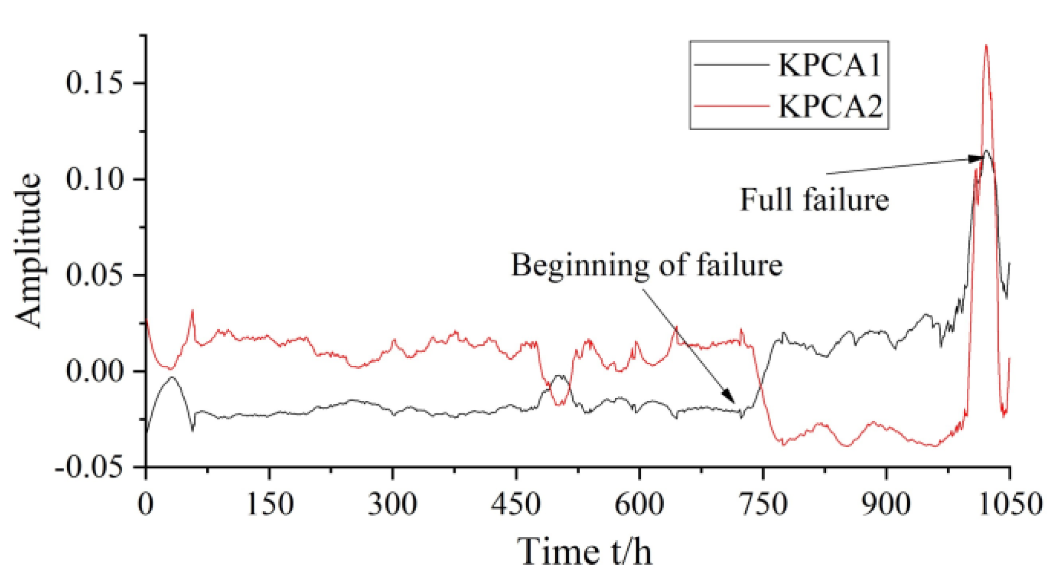
The KPCA method was used to perform the weighted fusion calculation of the selected characteristic parameters, and the first and second principal components were extracted as the evaluation indices representing the performance degradation of a gear pump. Subsequently, the RUL prediction model of a hydraulic pump based on KPCA and JITL was established using the RUL prediction method of JITL based on k-VNN.

The KPCA method was used to analyze the time- and frequency-domain characteristic parameters of the gear pump pressure signals. Based on Table 5, when the kernel parameter is $\sigma =450$, the CPVs of the first and second principal components of the four gear pumps exceed 90%. Therefore, in this study, the first and second principal components of tested gear pump 1–3 were selected as the training samples in the modeling. Moreover, the data of tested gear pump 4 were chosen as the test samples to verify the accuracy of the model.

As aforedescribed, the selected minimum neighborhood, $k_m$, and the weight factor, $\gamma$, in the JITL method have different effects on the predicted results. Among them, the maximum relative error (MRE) is listed in

Table 6. MREs of predicted results.

	γ	1.0	0.9	0.8	0.7	0.6	0.5
km
2		0.5340	0.7438	0.8205	0.8114	0.8114	0.8428
3		0.6644	0.7438	0.8205	0.8489	0.8495	0.8476
4		0.5681	0.7949	0.8243	0.8489	0.8495	0.8299
5		0.6184	0.7949	0.8243	0.8489	0.8495	0.8299
6		0.6184	0.8053	0.8243	0.8489	0.8495	0.8312
7		0.6192	0.8053	0.8243	0.8489	0.8495	0.8623

.

It can be observed from Table 6 that when the minimum neighborhood, $k_m$, is set as 2, 3, 4, and 5, respectively, the weight factors, $\gamma$, are 0.9 and 1.0; the corresponding MREs are smaller than the other MREs. To further optimize the values of the above parameters, the average relative errors (AREs) of the predicted results were compared, and the results are tabulated in

Table 7. AREs of predicted results.

	km	2	3	4	5
γ
0.9		15.8639	15.6194	15.4281	15.2987
1.0		15.9545	15.7997	15.3460	15.1547

.

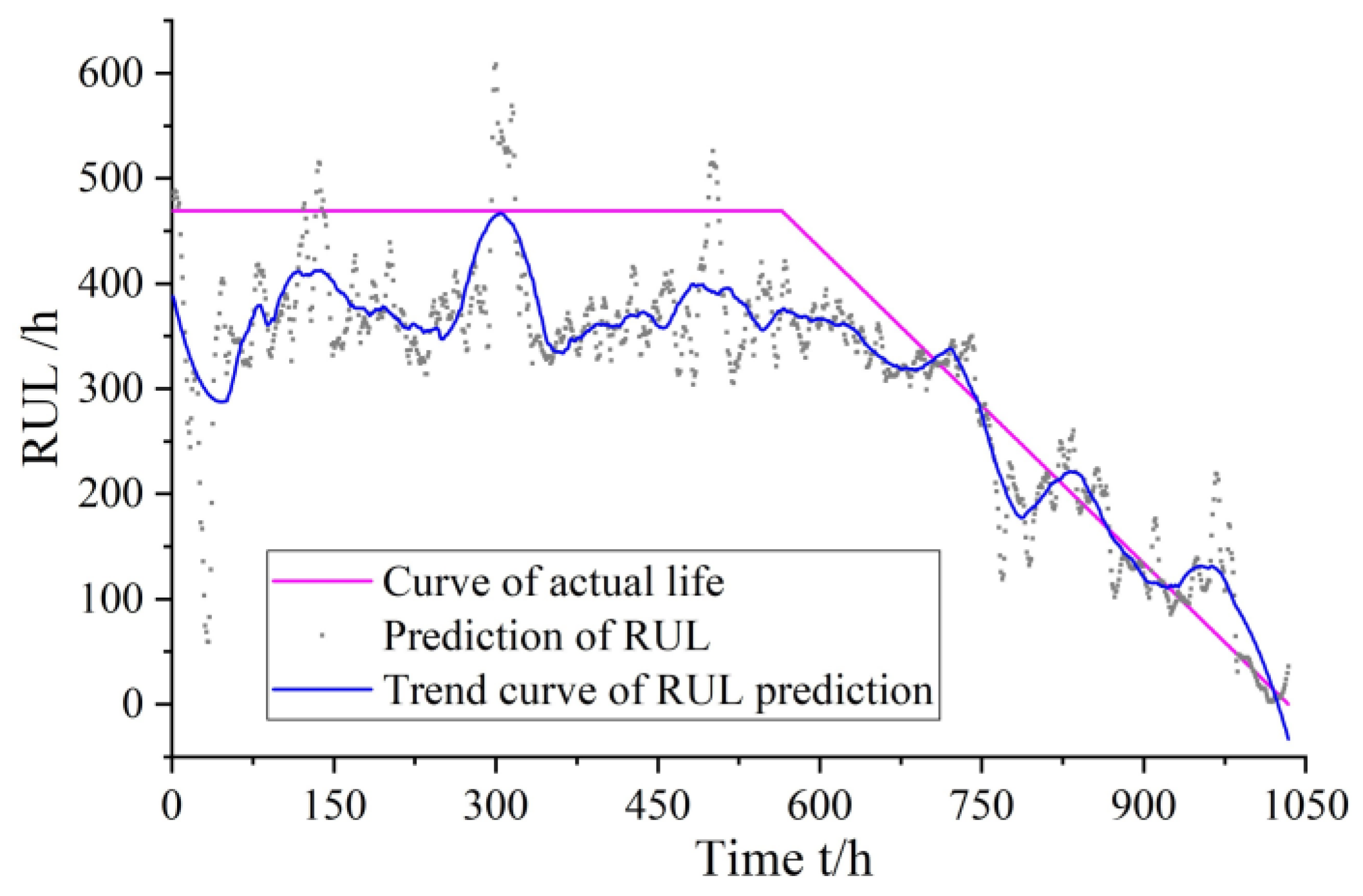
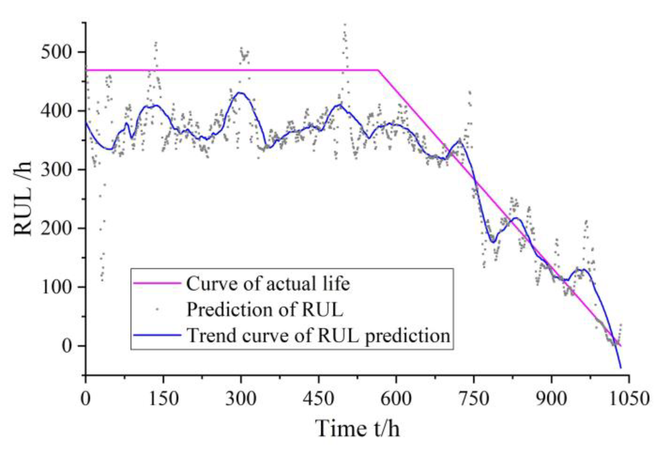
Based on Table 7, when minimum neighborhood $k_m=5$ and weight factor $\gamma =1.0$, the corresponding ARE is minimum. Therefore, in this study, parameters $k_m$ and $\gamma$ of the model established are 5 and 1.0, respectively. The model was established based on the life-cycle test data of gear pumps 1–3. The prediction results of the RUL of gear pump 4 obtained using the model are shown in Figure 11.

As can be seen from Figure 11, the gear pump is in a healthy state in the initial operating state without any mechanical failure; therefore, its life is not changed significantly. Over time, when the gear pump has operated for approximately 700 h, its RUL begins to decrease gradually. The predicted values of the RUL basically coincides with the real values.

To illustrate the RUL prediction efficiency of the JITL method proposed in this paper, the results are compared with those of the traditional JITL method based on k-NN, which are shown in Figure 12.

Table 8. Comparison of MRE and ARE of both methods.

Method	MRE	ARE
Proposed JITL method	0.6184	15.1547
JITL method based on k-NN	0.8962	16.2983

compares the MREs and AREs of both methods.

Table 8 indicates that both MRE and ARE of the gear pump RUL prediction method proposed in this paper are better than those of the traditional k-NN-based RUL prediction algorithm. The k-VNN method considers both the Euclidean distance and angle relationship between two vectors, while k-NN mainly refers to the Euclidean distance as the basis for modeling, which is insufficient for fully exploring the internal relationships among the input and nearest data. Therefore, sample selection method based on k-VNN of the RUL prediction method significantly improved the prediction accuracy of the RUL prediction model. This shows that the RUL prediction model based on KPCA and JITL proposed in this paper has higher prediction accuracy than the traditional RUL prediction model based on k-NN.

6. Conclusions

Aiming at the problem that the gear pump cannot be properly monitored and maintained in time, a mechanical equipment RUL prediction method based on the KPCA and JITL methods is proposed in this paper, which can timely warn the performance degradation process of the gear pump and timely forecast the RUL of the gear pump. It is used for the RUL prediction of gear pumps, and the prediction results show that the KPCA method can effectively extract their performance degradation indices. Simultaneously, the RUL prediction method based on JITL can effectively predict the RUL of the gear pumps. Compared to the traditional RUL prediction method, the method proposed herein exhibits a higher prediction accuracy. The method proposed in this paper is expected to be applied to the RUL prediction and condition monitoring of axial piston pumps, gearboxes, rolling bearings, and other components, and has broad application prospects and wide applicability.

• For obtaining the gear pump performance degradation evaluation indices, the characteristic parameters of the pressure signal include variance, root-mean-square value, peak value, root amplitude, peak-to-peak value, absolute mean value, standard deviation, shape factor, clearance factor, and average power, which have good sensitivity to the performance degradation of the gear pump. Using the KPCA method can effectively avoid the data redundancy caused by the correlations among various characteristic parameters. With continuous performance degradation of the gear pumps, the evaluation indices present a clear monotonic increasing trend. Simultaneously, the evaluation indices have good sensitivity to the early failure performance of the gear pumps.
• In the process of similar sample selection for the JITL method, the sample selection method based on k-VNN comprehensively considers the Euclidean distance and the angle between the information vectors, which can obviously reduce the MRE and ARE parameters of the RUL prediction method and significantly improve the prediction accuracy of the RUL prediction model. The feasibility and effectiveness of this method in the gear pump RUL prediction model are illustrated.
• The KPCA method and a k-VNN-based JITL method are combined and used for the RUL prediction of gear pumps. The method proposed in this paper is compared to the traditional k-NN-based JITL method. The results show that the RUL prediction model proposed in this paper has a higher prediction accuracy for the RUL prediction of gear pumps. The method proposed in this paper comprehensively considers multiple characteristic parameters of gear pump pressure signals, which are of great significance for improving the RUL prediction accuracy of a gear pump.

References

1. Song, Y.; Liu, J.; Chu, N.; Wu, P.; Wu, D. A novel demodulation method for rotating machinery based on time-frequency analysis and principal component analysis. J. Sound Vib. 2019, 442, 645–656. [Google Scholar] [CrossRef]
2. Zhou, R.; Jiao, Z.; Wang, S. Current research and developing trends on fault diagnosis of hydraulic systems. J. Mech. Eng. 2006, 42, 6–14. [Google Scholar] [CrossRef]
3. Jiang, W.; Li, Z.; Lei, Y.; Zhang, S.; Tong, X. Deep learning based rolling bearing fault diagnosis and performance degradation degree recognition method. J. Yanshan Univ. 2020, 44, 526–536. [Google Scholar] [CrossRef]
4. Siano, D.; Panza, M.A. Diagnostic method by using vibration analysis for pump fault detection. Energy Procedia 2018, 148, 10–17. [Google Scholar] [CrossRef]
5. Gajjar, S.; Kulahci, M.; Palazoglu, A. Real-time fault detection and diagnosis using sparse principal component analysis. J. Process Control 2018, 67, 112–128. [Google Scholar] [CrossRef]
6. Lei, Y.; Jia, F.; Kong, D.; Lin, J.; Xing, S. Opportunities and challenges of machinery intelligent fault diagnosis in big data era. J. Mech. Eng. 2018, 54, 94–104. [Google Scholar] [CrossRef]
7. Jiang, W.; Li, Z.; Li, J.; Zhu, Y.; Zhang, P. Study on a fault identification method of the hydraulic pump based on a combination of voiceprint characteristics and extreme learning machine. Processes 2019, 7, 894. [Google Scholar] [CrossRef] [Green Version]
8. Zhang, H.; Wang, S.; Zhang, Q.; Zhai, G. Research on fault diagnosis of rolling elements bearing based on wavelet packets transform. J. Vib. Shock 2004, 23, 127–131. [Google Scholar]
9. Choe, S.; Yoo, J. Wavelet Packet Transform Modulus-Based Feature Detection of Stochastic Power Quality Disturbance Signals. Appl. Sci. 2021, 11, 2825. [Google Scholar] [CrossRef]
10. Zhu, Y.; Jiang, W.; Kong, X. Adaptive extraction method for trend term of machinery signal based on extreme-point symmetric mode decomposition. J. Mech. Sci. Technol. 2017, 31, 493–500. [Google Scholar] [CrossRef]
11. Hu, A.; Ma, W.; Tang, G. Rolling bearing fault feature extraction method based on ensemble empirical mode decomposition and kurtosis criterion. Proc. CSEE 2012, 32, 106–111. [Google Scholar]
12. Jiang, W.; Zheng, Z.; Zhu, Y.; Li, Y. Demodulation for Hydraulic Pump Fault Signals Based on Local Mean Decomposition and Improved Adaptive Multiscale Morphology Analysis. Mech. Syst. Signal Proc. 2015, 58, 179–205. [Google Scholar] [CrossRef]
13. Naeem, K.; Kim, B.H.; Yoon, D.-J.; Kwon, I.-B. Enhancing Detection Performance of the Phase-Sensitive OTDR Based Distributed Vibration Sensor Using Weighted Singular Value Decomposition. Appl. Sci. 2021, 11, 1928. [Google Scholar] [CrossRef]
14. Huang, Y.; Wang, Y.; Luo, H.; Kong, D. New signal de-noising method based on fractional wavelet packet transform in time-frequency domain. Chin. J. Sci. Instrum. 2011, 32, 1534–1539. [Google Scholar]
15. Su, X.; Li, H. Denoising of shock signal based on EMD and wavelet threshold. Comput. Meas. Control 2017, 25, 204–208. [Google Scholar]
16. Tang, Y.; Sun, Q. Study on vibration signal singularity analysis by wavelet for rolling element bearing defect detection. J. Vib. Eng. 2002, 15, 111–113. [Google Scholar]
17. Yi, C.; Wang, X.; Zhu, Y.; Ke, W. A Novel Adaptive Mode Decomposition Method Based on Reassignment Vector and Its Application to Fault Diagnosis of Rolling Bearing. Appl. Sci. 2020, 10, 5479. [Google Scholar] [CrossRef]
18. Zhang, G.; Song, L.; Zhang, X.; Sun, Z.; Liang, H.; Xiao, Z.; Cheng, Y. Research on method of hydroelectric generating unit vibration signal de-noising based on multiwavelets. China Rural Water Hydropower 2016, 5, 163–170. [Google Scholar]
19. Xuan, Y.; He, L.; Chen, Z.; Liao, J. Fault feature extraction method of hydraulic pump based on pulsating pressure signal. J. Nav. Univ. Eng. 2020, 32, 108–112. [Google Scholar]
20. Wang, L.; Wu, X.; Zhang, C.; Shi, H. Hydraulic system fault diagnosis method based on a multi-feature fusion support vector machine. J. Eng. 2019, 13, 215–218. [Google Scholar] [CrossRef]
21. Wang, P.; Wang, X.; Zhu, H.; Li, Y.; Zhang, M. A fault diagnosis method based on sparse coding for hydraulic pump. Trans. Beijing Inst. Technol. 2017, 37, 451–454. [Google Scholar]
22. Su, W. Research on Rolling Element Bearing Vibration Signal Processing and Feature Extraction Method. Ph.D. Thesis, Dalian University of Technology, Dalian, China, 2010. [Google Scholar]
23. Zheng, Z.; Jiang, W.; Wang, Z.; Zhu, Y.; Yang, K. Gear Fault Diagnosis Method Based on Local Mean Decomposition and Generalized Morphological Fractal Dimensions. Mech. Mach. Theory 2015, 91, 151–167. [Google Scholar] [CrossRef]
24. He, Z.; Zi, Y.; Zhang, Z.; Ma, J.; Gao, Q.; Yang, S. Key technologies on dynamic analysis and monitoring-diagnosis of varying operation and nonstationarity for large mechanical equipment. China Mech. Eng. 1999, 10, 978–981. [Google Scholar]
25. Zhao, Y.; Wang, Y. Remaining useful life prediction for multi-sensor systems using a novel end-to-end deep-learning method. Measurement 2021, 182, 109685. [Google Scholar] [CrossRef]
26. Hotait, H.; Chiementin, X.; Rasolofondraibe, L. Intelligent Online Monitoring of Rolling Bearing: Diagnosis and Prognosis. Entropy 2021, 23, 791. [Google Scholar] [CrossRef] [PubMed]
27. Wang, M.; Zhang, Z.; Li, K.; Si, C.; Li, L. Survey on Advanced Equipment Fault Diagnosis and Warning Based on Big Data Technique. J. Stat. Mech. Theory Exp. 2020, 1549, 042134. [Google Scholar] [CrossRef]
28. Tan, Y.; Zhang, C.; Chen, X.; Wang, Y. Remaining life evaluation based on accelerated life testing. J. Mech. Eng. 2010, 46, 150–154. [Google Scholar] [CrossRef]
29. Sim, J.; Kim, S.; Park, H.J.; Choi, J.-H. A Tutorial for Feature Engineering in the Prognostics and Health Management of Gears and Bearings. Appl. Sci. 2020, 10, 5639. [Google Scholar] [CrossRef]
30. Kong, G.; Zhang, P.; Qian, L.; Wu, F. A new evaluation method for residual life of gun. J. Ballist. 2010, 22, 21–25. [Google Scholar]
31. Li, X.; Mba, D.; Lin, T.; Yang, Y.; Loukopoulos, P. Just-in-Time Learning Based Probabilistic Gradient Boosting Tree for Valve Failure Prognostics. Mech. Syst. Signal Process. 2021, 150, 107253. [Google Scholar] [CrossRef]
32. Bontempi, G.; Birattari, M.; Bersini, H. Lazy Learning for Local Modelling and Control Design. Int. J. Control 1999, 72, 643–658. [Google Scholar] [CrossRef]
33. Su, Q.-L.; Hermanto, M.W.; Braatz, R.D.; Chiu, M.-S. Just-in-Time-Learning Based Extended Prediction Self-Adaptive Control for Batch Processes. J. Process Control 2016, 43, 1–9. [Google Scholar] [CrossRef]
34. Jin, H.; Chen, X.; Yang, J.; Wu, L. Adaptive Soft Sensor Modeling Framework Based on Just-in-Time Learning and Kernel Partial Least Squares Regression for Nonlinear Multiphase Batch Processes. Comput. Chem. Eng. 2014, 71, 77–93. [Google Scholar] [CrossRef]
35. Wang, L.; Sun, Y.; Yang, K.; Liu, X.; Chen, X. A soft sensor method based on just in time learning and multi-mode ensemble GPR. Trans. Beijing Inst. Technol. 2018, 38, 196–199. [Google Scholar]
36. Qi, C.; Shi, X.; Xiong, W. A just-in-time learning soft sensor modeling method based on the second-order similarity. CAAI Trans. Intell. Syst. 2020, 15, 910–918. [Google Scholar]
37. Jin, H.; Pan, B.; Chen, X.; Qian, B. Ensemble Just-in-Time Learning Framework through Evolutionary Multi-Objective Optimization for Soft Sensor Development of Nonlinear Industrial Processes. Chemom. Intell. Lab. Syst. 2019, 184, 153–166. [Google Scholar] [CrossRef]
38. Guo, F.; Xie, R.; Huang, B. A Deep Learning Just-in-Time Modeling Approach for Soft Sensor Based on Variational Autoencoder. Chemom. Intell. Lab. Syst. 2020, 197, 103922. [Google Scholar] [CrossRef]
39. Zheng, Z.; Jiang, W.; Zhu, Y.; Hu, H. Application of morphological difference filter and morphological index to wear condition assessment of hydraulic pump slipper. J. Vib. Shock 2015, 34, 13–17. [Google Scholar]
40. Tenekedjiev, K.; Abdussamie, N.; An, H.; Nikolova, N. Regression Diagnostics with Predicted Residuals of Linear Model with Improved Singular Value Classification Applied to Forecast the Hydrodynamic Efficiency of Wave Energy Converters. Appl. Sci. 2021, 11, 2990. [Google Scholar] [CrossRef]
41. Liu, Y.; Li, H.; Wang, Z. The mechanical fault prediction based on wavelet neural network. J. Mech. Transm. 2006, 30, 68–70. [Google Scholar]
42. Muin, S.; Mosalam, K.M. Structural Health Monitoring Using Machine Learning and Cumulative Absolute Velocity Features. Appl. Sci. 2021, 11, 5727. [Google Scholar] [CrossRef]
43. Zhu, X. Fault diagnosis of rolling bearing based on kernel principal component analysis and naive bayes. Mod. Comput. 2019, 9, 18–22. [Google Scholar]
44. Vapnik, V. Statistical learning theory. Encycl. Sci. Learn. 1998, 41, 3185. [Google Scholar]
45. Cheng, C.; Chiu, M.-S. A New Data-Based Methodology for Nonlinear Process Modeling. Chem. Eng. Sci. 2004, 59, 2801–2810. [Google Scholar] [CrossRef]
46. Cao, H.; Guo, Q. Multi aspects analysis and application of least square method. Stud. Coll. Math. 2019, 22, 47–49. [Google Scholar]
47. Chinniah, Y.; Burton, R.; Habibi, S. Failure Monitoring in a High Performance Hydrostatic Actuation System Using the Extended Kalman Filter. Mechatronics 2006, 16, 643–653. [Google Scholar] [CrossRef]
48. Shi, Z. Excitation Controller Using Iterative Learning Control Based on Lazy Learning Method. Master’s Thesis, Lanzhou University of Technology, Lanzhou, China, 2010. [Google Scholar]
49. Sun, W.; Wang, W.; Zhu, R. Iterative learning control for nonlinear system using lazy learning method. Control Decis. 2003, 18, 263–266. [Google Scholar]
50. Zhang, G. The Pr/Nd Extraction Process Component Content Prediction Based on JIT Learning. Master’s Thesis, East China Jiaotong University, Nanchang, China, 2017. [Google Scholar]
51. Zheng, C. Estimate on the invalid rate of nonsubstitute time tac-tail life experiment of index distribution. J. Jingdezhen Coll. 2000, 15, 37–39. [Google Scholar]
52. Liang, G.; Xue, J.; Hu, L.; Cao, K. Fuzzy pattern recognition of constant displacement pump life distribution based on timing censored life test. Mach. Tool Hydraul. 2014, 42, 159–162. [Google Scholar]
53. Xue, D. Research on Prediction Method of Gear Pump Remaining Life Based on Real-Time Learning. Master’s Thesis, Yanshan University, Qinhuangdao, China, 2020. [Google Scholar]
Figure 1. The RUL prediction process of gear pump.
Applsci 11 09389 g001
Figure 2. Comparison of wavelet decomposition and wavelet packet decomposition: (a) Wavelet decomposition and (b) Wavelet packet decomposition.
Applsci 11 09389 g002
Figure 3. Life-cycle test bed of gear pump: (a) Topside of test bed and (b) Underside of test bed.
Applsci 11 09389 g003
Figure 4. Hydraulic system schematic of gear pump life-cycle test bed: 1—Tank; 2—Liquid thermometer; 3—Return oil filter; 4—Forced-air cooler; 5—Air filter; 6—Self suction oil filter; 7—Electric motor; 8—Gear pump; 9—High-pressure hose; 10—Relief valve; 11—Pressure gauge; 12—Flow meter; 13—Valve block; 14—Electromagnetic reversing valve; 15—High pressure filter; 16—Pressure sensor; 17—Torque-speed transducer; and 18—Temperature sensor.
Applsci 11 09389 g004
Figure 5. Schematic of step-stress acceleration degradation test.
Applsci 11 09389 g005
Figure 6. Volumetric efficiency degradation curves of gear pumps.
Applsci 11 09389 g006
Figure 7. Wear of each component of gear pump: (a) End-face wear of driving gear; (b) End-face wear of driven gear; (c) Side plate wear; and (d) Pump body wear.
Applsci 11 09389 g007
Figure 8. Time-domain characteristic parameters: (a) Mean value; (b) Variance; (c) Root-mean-square value; (d) Kurtosis; (e) Peak value; (f) Root amplitude; (g) Peak-to-peak value; (h) Absolute mean value; (i) Standard deviation; (j) Shape factor; (k) Crest factor; (l) Impulse factor; (m) Kurtosis index; and (n) Clearance factor.
Applsci 11 09389 g008aApplsci 11 09389 g008b
Figure 9. Frequency-domain characteristic parameters: (a) Gravity frequency; (b) Mean square frequency; (c) Frequency variance; and (d) Average power.
Applsci 11 09389 g009
Figure 10. First and second principal components obtained by KPCA method.
Applsci 11 09389 g010
Figure 11. RUL prediction of gear pump 4 based on JITL method proposed in this paper.
Applsci 11 09389 g011
Figure 12. RUL prediction of gear pump 4 predicted by JITL method based on k-NN.
Applsci 11 09389 g012