Article

Protective Measurement—A New Quantum Measurement Paradigm: Detailed Description of the First Realization

1
Istituto Nazionale di Ricerca Metrologica, Strada Delle Cacce 91, I-10135 Torino, Italy
2
Politecnico di Milano, Dipartimento di Elettronica, Informazione e Bioingegneria, Piazza Leonardo da Vinci 32, I-20133 Milano, Italy
3
Faculty of Engineering and the Institute of Nanotechnology and Advanced Materials, Bar Ilan University, Ramat Gan 5290002, Israel
4
Raymond and Beverly Sackler School of Physics and Astronomy, Tel-Aviv University, Tel-Aviv 6997801, Israel
5
INFN, Sez. di Torino, Via P. Giuria 1, I-10125 Torino, Italy
*
Author to whom correspondence should be addressed.
Appl. Sci. 2021, 11(9), 4260; https://doi.org/10.3390/app11094260
Submission received: 31 March 2021 / Revised: 25 April 2021 / Accepted: 6 May 2021 / Published: 8 May 2021
(This article belongs to the Special Issue Quantum Optics for Fundamental Quantum Mechanics II)

Abstract

:
We present a detailed description of the experiment realizing for the first time a protective measurement, a novel measurement protocol which combines weak interactions with a “protection mechanism” preserving the measured state coherence during the whole measurement process. Furthermore, protective measurement allows finding the expectation value of an observable, i.e., an inherently statistical quantity, by measuring a single particle, without the need for any statistics. This peculiar property, in sharp contrast to the framework of traditional (projective) quantum measurement, might constitute a groundbreaking advance for several quantum technology related fields.

1. Introduction

Measurement in quantum mechanics is usually described through projective measurements (PJs), represented by a projector onto physical states within a given Hilbert space. This kind of measurement induces the wavefunction collapse onto a specific eigenstate of the observable, corresponding to the observed eigenvalue. In contrast with this measurement paradigm, in weak measurements, introduced by Aharonov, Albert and Vaidman [1], the coupling between the pointer and the quantum state is weak, introducing only a partial decoherence of the wavefunction, at the price of acquiring only partial information about the state. Examples of weak-coupling-based schemes are measurements of weak values [1,2] and protective measurements (PMs) [3,4,5,6].
In general, a common property for all quantum measurements is that the measurement procedure is invasive, inducing unavoidable decoherence in the initial state of the system. Even in weak value measurements [1,2,7,8,9,10,11,12,13,14,15,16,17,18,19,20,21,22,23,24,25,26,27,28,29,30,31,32,33,34,35,36,37,38,39,40], the coupling between the system and the measuring device causes a small perturbation to the system state. In contrast to other quantum measurement paradigms, a PM is able to preserve the coherence of the quantum state during the whole measurement process, thanks to a protection mechanism or alternatively, via the adiabatic theorem [3]. This difference with respect to traditional measurement protocols allows the PM to extract the expectation value of an observable (thus far considered an inherently statistical quantity, only obtainable by means of repeatedly measuring an ensemble of identically prepared systems) by measuring a single quantum system.
Hence, PM is a novel measurement paradigm presenting significant elements of interest, both as a tool for quantum metrology and for understanding the very foundations of quantum measurement, and more generally, of quantum mechanics itself, e.g., the possibility of measuring a stationary wavefunction | ψ [3]. For this reason, on the one hand, PMs add significant elements to the debate about the ontic or epistemic nature of the wavefunction, a highly debated topic in the scientific community [4,5,6,41,42,43,44,45,46,47,48,49,50,51,52,53,54,55,56], and on the other hand, they allow overcoming the quantum Cramér–Rao bound in specific protocols [57,58].
In this work, we extensively illustrate the scheme, methodology and obtained results related to the first experimental implementation of PM [57], demonstrating its capability to preserve the system state coherence, and at the same time, extract the expectation value of an observable even from a single measurement event.

Theoretical Framework

In the framework of quantum mechanics, given a quantum state | ψ , we define the quantum expectation value of an observable A = i a i | ϕ i ϕ i | (with i | ϕ i ϕ i | = I ) as the average of its eigenvalues a i weighted on their respective probabilities p i :
A = ψ | A | ψ = i p i a i p i = | ψ | ϕ i | 2
Similarly to its classical counterpart, A is understood as a statistical property.
PM can be modeled as a standard von Neumann measurement [59] in which we couple the observable of interest A with a pointer P with a long and adiabatic interaction instead of the usual instantaneous one. Such interactions are mediated by the coupling g ( t ) , which allows us to write the interaction Hamiltonian as
H i n t = g ( t ) A P
where the interaction intensity is g ( t ) = g / T for a time interval T and smoothly goes to zero before and after. If the coupling g ( t ) is smooth enough, we obtain the adiabatic limit, in which the state of the system | ψ does not change, thanks to the protection. In the limit T and for bounded P, one has H i n t 0 while the state | ψ remains unchanged thanks to the preserving action of the protection mechanism. We can calculate, then, the shift of the energy of the eigenstate via first-order perturbation theory [3]:
δ E H i n t = g A P T
from which we can calculate the time evolution U associated to H i n t in the limit T :
U exp i g A P
resulting in a pointer wavefunction shift proportional to the expectation value A .
A second protection scheme involves the so-called active protection, based on the quantum Zeno effect [60], which consists of a series of repeated projections onto the initial state [61,62,63,64,65,66,67,68,69,70,71,72,73,74,75,76,77,78,79,80] during the interaction described by the Hamiltonian in Equation (2), but in the non-adiabatic limit. In our experiment, we will focus on this quantum Zeno-type protection [6].
From a quantum informational perspective, our experiment corresponds to a protocol in which Alice produces a quantum state, which she transmits to Bob together with the proper protection, implemented by Bob as a black box when realizing the PM.
The PM framework can be formalized with an equivalent description consisting of a series of K instantaneous weak interactions, described by a (weak) coupling constant g = t = 0 T g ( t ) d t . Between two subsequent interactions, the active protection occurs, induced by the projector Π ψ = | ψ ψ | . It is straightforward to show that, in the weak interaction approximation ( g 1 ), each of the K weak interaction/protection blocks evolves the system in the following way:
| ψ ψ | U | ψ | φ ( x ) = | ψ ψ | exp i g A P | ψ | φ ( x ) | ψ | φ ( x g A ^ )
where | φ ( x ) is the pointer initial wavefunction.
From Equation (5), one can see how the PM induces a shift in the meter wavefunction, which is directly proportional to the expectation value A . PMs, then, allow us to directly estimate the expectation value A for each single particle undergoing them, in sharp contrast with the concept of A being only a statistical quantity.

2. Experimental Implementation
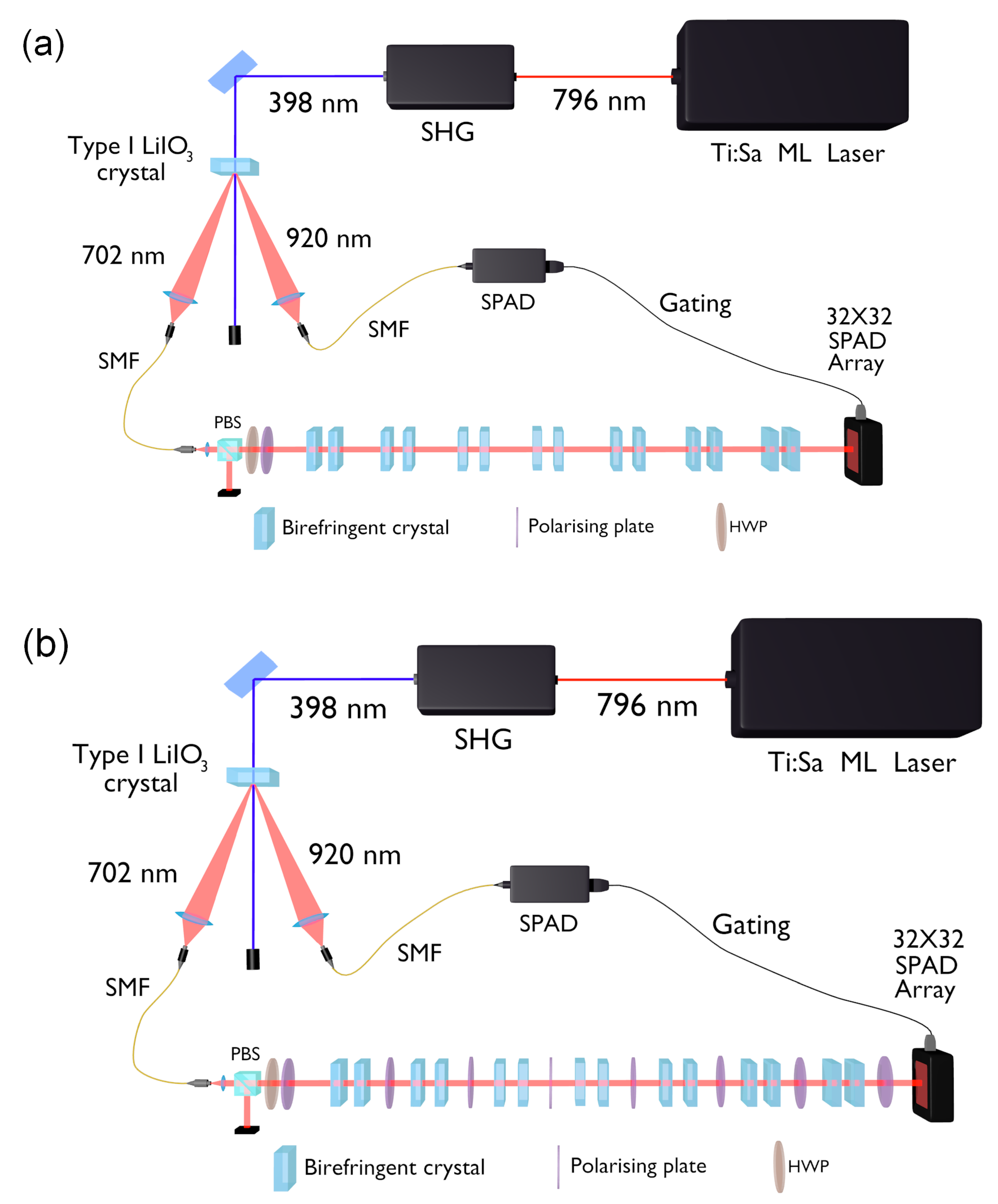
In our experiment, we implement two different methods to measure the expectation value of the polarization operator A = | H H | | V V | (with H and V being the horizontal and vertical polarization, respectively): the aforementioned PM, able to estimate A with a single reading of the measuring device, and a traditional PJ, in which the expectation value is extracted from the statistics obtained from repeated measurements on an ensemble of identically prepared particles. Both measurements can be described as a von Neumann protocol in which we couple the polarization of an incoming photon, prepared in the linearly polarized state | ψ = cos ( θ ) | H + sin ( θ ) | V , with its transverse momentum P :
U = exp i g Π H P
where Π H = | H H | is the projector onto the H polarization. This interaction causes a shift of the horizontally polarized component of the wavefunction along an axis orthogonal to the photon propagation direction. This is mathematically equivalent to a von Neumann coupling of strength g / 2 between the polarization A and the momentum P , so from here we will consider a rescaling of our system in order to describe the latter scenario.
The initial spatial wavefunction of the photon is described by a normal distribution:
ϕ 0 ( x ) = x | ϕ 0 = 1 2 π σ 2 4 exp ( x x 0 ) 2 4 σ 2 ,
centered at x 0 and with standard deviation σ .
For strong interactions (i.e., g 1 ), the two polarization components will be completely separated (Figure 1a). Hence, the expectation value can be evaluated as
A = N H N V N H + N V
where N H ( V ) is the number of count events obtained for the polarization H(V). This is the case of projective measurement [81].
PMs, instead, in our scheme, consist of a series of weak von Neumann couplings ( g 1 ) alternating with a protection mechanism, i.e., a projection Π ψ = | ψ ψ | onto the initial state | ψ . In this case, the photons will fall in a region not corresponding to any eigenvalue of our polarization observable A, but whose position is directly proportional to its expectation value (Figure 1b). Thus, the expectation value of the polarization can be extracted by the formula:
A = x x 0 a
with x 0 = x H + x V 2 and a = x H x V 2 , being x H ( x V ) the center of the horizontally (vertically) polarized photon distribution in the PJ framework.

Experimental Setup

Both PM and PJ experimental setups (Figure 2a,b, respectively) can be divided into three parts.
In the first part, single photons are generated by a heralded single-photon source [82,83]. A mode-locked laser with a second harmonic at 398 nm and a 76 MHz repetition rate pumps a 10 × 10 × 5 mm LiIO 3 non-linear crystal, producing signal–idler photon pairs by exploiting Type-I spontaneous parametric down-conversion (SPDC). The generated idler photons (920 nm) are filtered by an interference filter (IF) centered at 920 nm and with a FWHM of 10 nm, coupled to a single-mode fiber(SMF) which addresses them to a Silicon single-photon avalanche diode (SPAD), heralding the presence of the correlated signal photons (702 nm). Signal photons are filtered with an IF centered at 702 nm and with a FWHM of 10 nm, fiber-coupled and addressed to the second part of the setup, where the PM takes place. A Hanbury–Brown and Twiss interferometer allowed us to estimate the quality of our single-photon emission by evaluating the α parameter [84,85], obtaining a value of α = 0.13 ± 0.01 without any background or dark count subtraction, testifying the high quality of our heralded single-photon source.
In the second part, the PM and PJ are performed. The signal photon produced in the previous stage is decoupled and collimated in a Gaussian spatial mode over a 2 m length. Then, it is initialized (pre-selected) in the polarization state | ψ by a polarizing beam splitter (PBS) followed by a half-wave plate (HWP). Finally, in the PJ configuration (Figure 2a), the photon goes through K = 7 weak interaction units (we chose the number of units K = 7 from practical considerations approximating the ideal case of large K). Each unit consists of a first 2 mm-long birefringent calcite crystal with an extraordinary (e) optical axis lying in the xz plane, having an angle of π / 4 with respect to the z direction, followed by a second 1.1 mm calcite crystal with the optical e-axis oriented along the y-axis. The first crystal shifts the horizontally polarized component of the wavefunction along the transverse direction x, while the second one compensates for the phase and time decoherence induced by the first crystal. The combined effect of all the seven units allows for the complete separation of orthogonal polarizations, reproducing the PJ framework. In the PM scenario (Figure 2b), instead, the protection of the quantum state is implemented, exploiting the quantum Zeno effect, realized by inserting a polarizing plate after each weak interaction unit. The polarizing plate realizes the projection Π ψ = | ψ ψ | , projecting the state outgoing the weak von Neumann interaction onto the same polarization of the initial state | ψ , thus canceling the (small) decoherence induced by the birefringent crystals in each weak interaction unit.
The final part of each experimental setup is the detection stage: photons are detected by a 2D spatially resolving single-photon detector prototype, i.e., a two-dimensional array of 32 × 32 “smart pixels”, each hosting a SPAD with dedicated front–end electronics [86]. The detection of the idler photon (920 nm) by the Si-SPAD on the heralding arm gates the SPAD array with a 6 ns detection window.
Furthermore, an optional quantum tomography [87,88] apparatus, comprising an HWP, a quarter-wave plate (QWP) and a polarizer, can be inserted just before the SPAD array to reconstruct the density matrix of the single-photon state at the end of each measurement procedure.

3. Results

We acquired data sets for three different states: the state | + = 1 2 ( | H + | V ) , which should be subjected to the maximum decoherence, and the intermediate states | π 8 = cos ( π 8 ) | H + sin ( π 8 ) | V and | 17 60 π = cos ( 17 60 π ) | H + sin ( 17 60 π ) | V . Each data set is composed of multiple acquisitions:
  • An acquisition with only the crystals in the optical path and | ψ = | H or | ψ = | V , which allows us to calibrate the system;
  • An acquisition without protection (only crystals in the optical path), corresponding to the traditional PJ scenario;
  • An acquisition with both weak interaction and active Zeno-like protection (both birefringent crystals and polarizers in the optical path), realizing the PM;
  • Two acquisitions, one with only the polarizing plates and one with a free optical path, allowing us to complete the system calibration by evaluating and properly subtracting unwanted position biases introduced by crystals and polarizing plates.

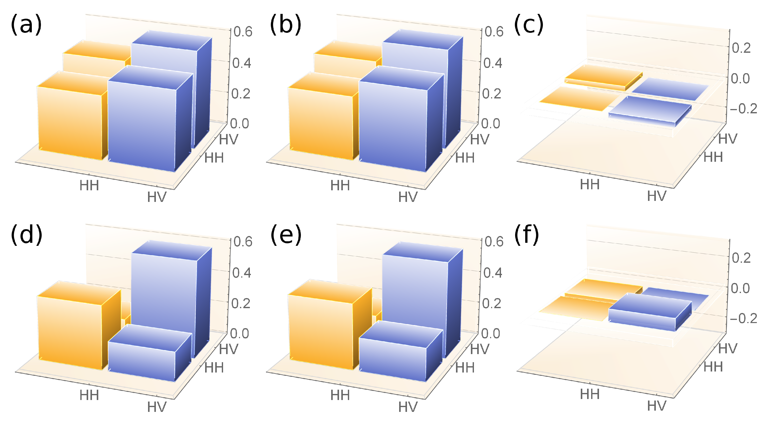
3.1. Output State Verification

To immediately highlight the difference between PM and PJ, we performed a tomographic reconstruction of the states at the end of the measurement process.
In the PJ case, we expected that the repeated shifts of the horizontal polarization component would cause decoherence on ρ ^ i n = | ψ ψ | , generating a final state ρ ^ d e c . In contrast, in the PM case, the protection should be able to preserve, in principle, the initial polarization state ρ ^ i n , thus we expect a final state ρ ^ p r o t = ρ ^ i n :
ρ ^ i n = cos 2 ( θ ) sin ( θ ) cos ( θ ) sin ( θ ) cos ( θ ) sin 2 ( θ )
ρ ^ d e c = cos 2 ( θ ) sin ( θ ) cos ( θ ) exp g 2 ( 2 σ ) 2 sin ( θ ) cos ( θ ) exp g 2 ( 2 σ ) 2 sin 2 ( θ )
where g = x H x V = 11.56 ± 0.07 px (pixels), as x H ( V ) is the average position of photons in the H ( V ) polarization on the x axis, and σ = 4.17 ± 0.02 px is the distribution width obtained by Gaussian fits.
We first computed the distance between the reconstructed states ρ P M r e c and ρ P J r e c , respectively, obtained in the PM and PJ case (shown in Figure 3 for the state | 17 60 π ), and their theoretical counterparts ρ i n and ρ d e c , by evaluating the Fidelity F [89,90] between them (second and third columns of the Table 1). The high fidelities obtained certify the adherence of the experimental results to our model, showing that PM indeed preserves the initial state by the decoherence induced by the birefringent crystals, while this does not happen for PJ.
Then, we compute the distance between the two reconstructed states (fourth column of Table 1). Again, the low fidelities obtained tell us that, without protection, the decoherence induced on the initial state by the K = 7 unitary interactions makes the final state totally incompatible with the one outgoing the PM procedure (and, obviously, with the initial state itself).
Finally, by analyzing the purity P [89] of the reconstructed states (last two columns of Table 1), we notice that, as expected, the decoherence reduced the purity of the initial state ρ i n in the PJ case, while this does not happen in the PM one. Thus, we proved the PM protocol’s ability to preserve the coherence of the initial state during the whole measurement process, a feature in sharp contrast with the traditional quantum measurement paradigms.

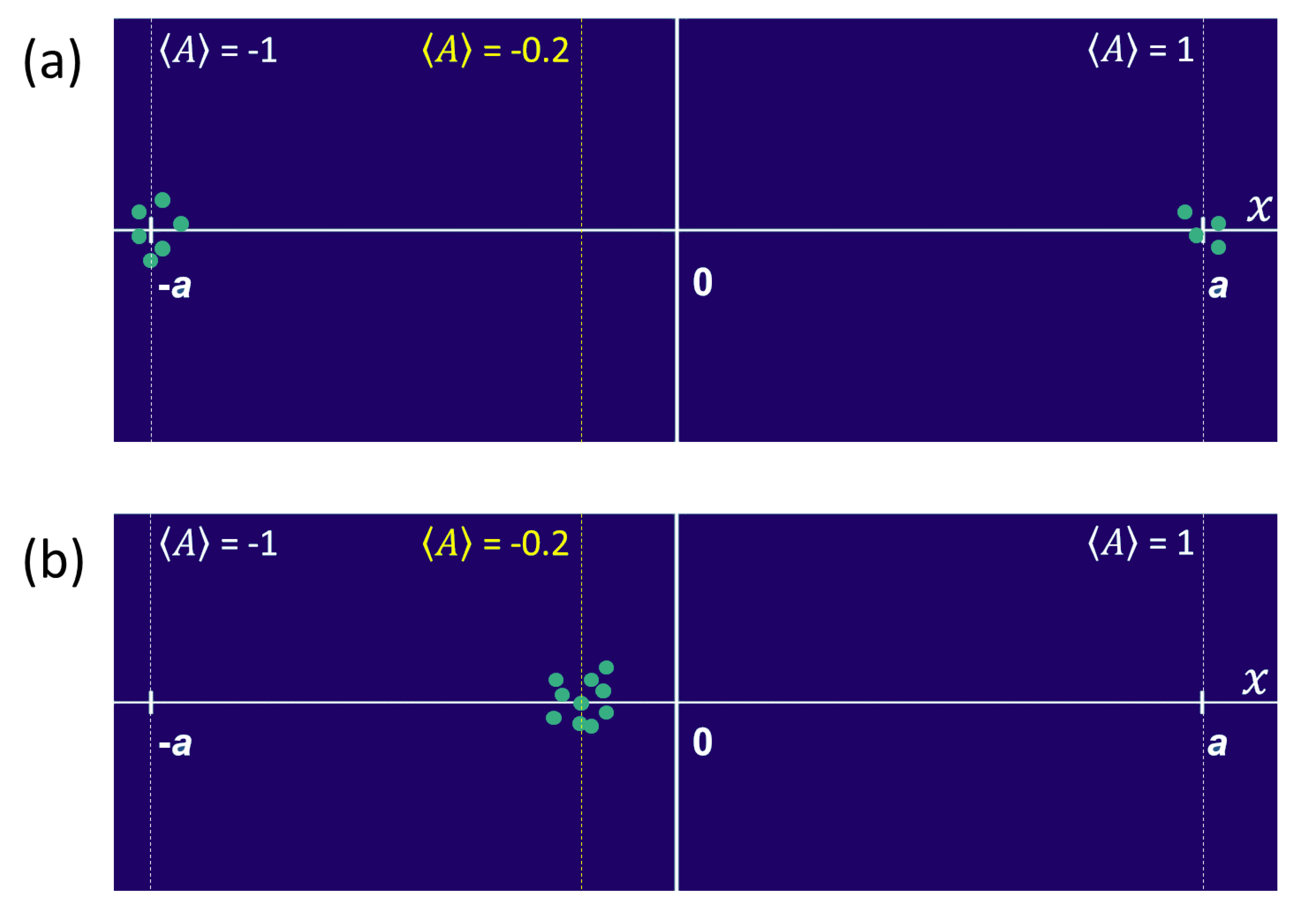
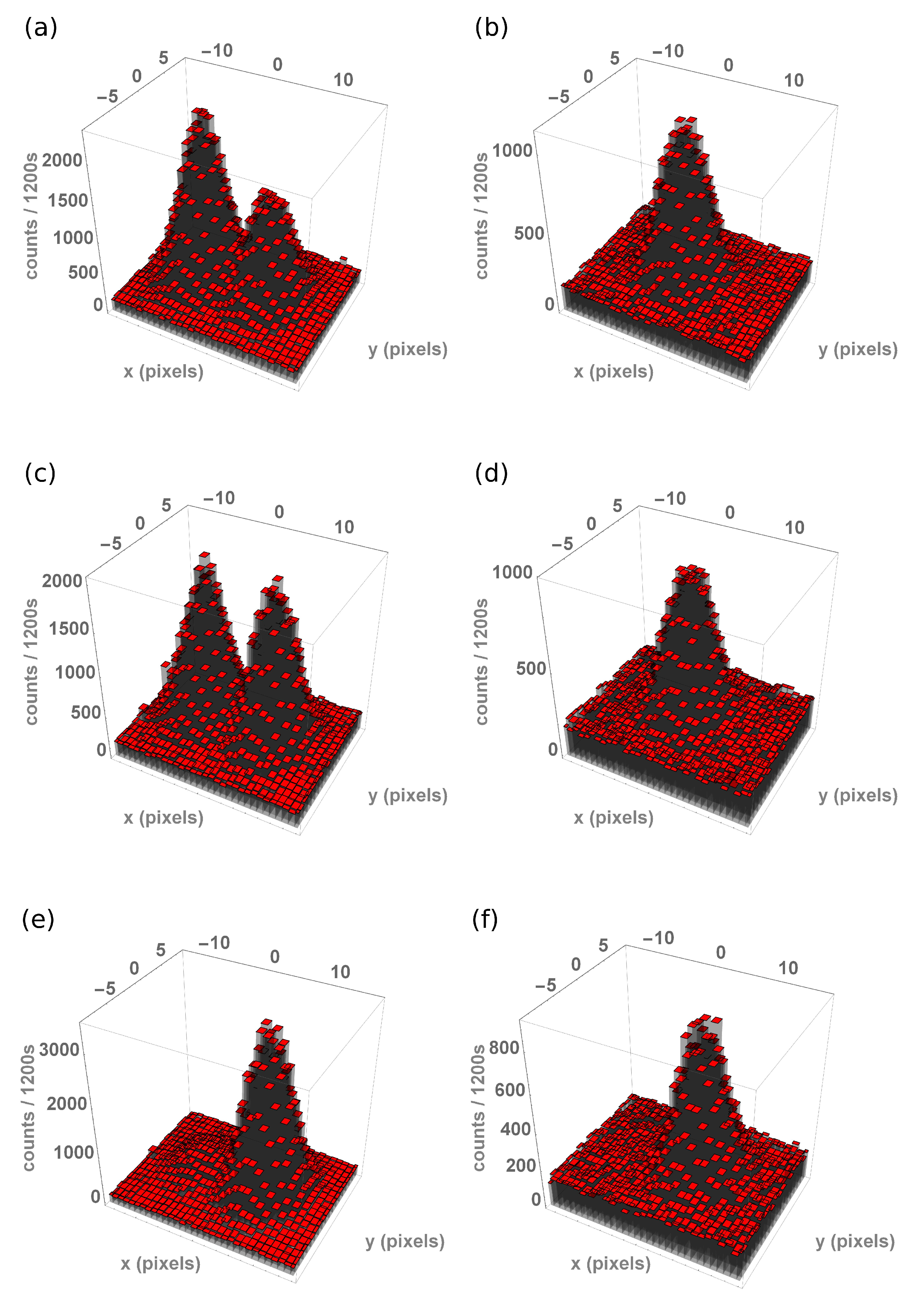
3.2. Expectation Values

Subsequently, in order to test the predictions of PM regarding the possibility of extracting the expectation value A even from a single detection event, we evaluated A with both the PM and PJ methods.
Plots in Figure 4a,c,e show the results obtained for the three states in the PJ case. We can see that the photons accumulate around the two eigenvalues’ positions x H and x V , hence, we can statistically find the expectation value as the counts ratio in Equation (8).
Plots in Figure 4b,d,f host, instead, the PM results, in which all the photons accumulate in a specific position corresponding to x = a A , in agreement with our expectations. This is clear evidence that, with PM, each single photon carries information about the expectation value of its polarization.
The extracted expectation values are reported in Table 2, column 3 for PJ and in Table 2, column 4 for PM, together with the associated experimental uncertainties (a detailed description of the expectation values and uncertainties analysis can be found in Appendix A). Within the experimental uncertainties, the expectation values extracted with the PM method are in good agreement with the ones obtained with the traditional PJ one, as well as with the theoretical expectations.
In [57], a general comparison was performed between the uncertainties associated with the PM and PJ protocols (considering the same amount of initial photons), showing how PM performs better than PJ in terms of precision for almost every initial state.
To further confirm this result, the two plots in Figure 5 show the equivalent of the distributions in Figure 4a,b for a few detection events. However, for the PM in Figure 5b, all the counts (except for dark counts) belong to a region centered in the x axis position corresponding to the expectation value A , though the same does not happen for the PJ in Figure 5a. Henceforth, with PM, one can achieve a sound estimate of the average polarization value for the state | 17 60 π from just the first detection event (yellow pixel in Figure 5b), obtaining A = 0.3 ± 0.3 , where the uncertainty is estimated from the width of the initial (Gaussian) spatial photon distribution. This result is in agreement with the theoretically expected value A th = 0.208 . On the contrary, it is not possible to do the same in the PJ case, since the first detection event (yellow pixel in Figure 5a) does not provide any reliable information about the expectation value of the detected photon polarization. This is a final demonstration of the PM capability of extracting the expectation value even from a single detection event.

4. Conclusions

Protective measurements represent a novel, groundbreaking measurement paradigm, which allow preserving the initial coherence of the measured state and extracting the expectation value of an observable, to date considered as a purely statistical quantity, even from a single detection event. The presented results demonstrate this unprecedented capability by exploiting certified single photons. In particular, in this paper, we described in detail the first experimental implementation of PM, providing the readers with all the details needed for a full understanding of the experiment and obtained results, as well as of the related implications for quantum mechanics foundations. We verified that PM preserves the coherence of the initial state during the whole measurement process, as certified by the high fidelities between the initially prepared states and the reconstructed ones outgoing the PM. Furthermore, the ability of PM to extract the expectation value of a quantum observable from a single (protected) particle is demonstrated by the photon distributions obtained with this protocol, always centered in a position proportional to the expectation value of the polarization of the detected photons and allowing to estimate the polarization expectation values always in agreement with the ones obtained with traditional PJ, all matching the theoretical expectations within the experimental uncertainties.
These results shed important insight on the very foundations of quantum mechanics, especially in the long-standing debate about the ontic or epistemic nature of the wavefunction, at the same time paving the way toward new quantum measurement methods with possible significant application for quantum technologies, and in particular, to quantum metrology [91,92,93], with the eventual possibility to exceed the quantum Cramér–Rao bound [94] thanks to the parameter dependence of the measurement procedure [95,96].

Author Contributions

Conceptualization, E.C., I.P.D., L.V., M.G. (Marco Genovese) and M.G. (Marco Gramegna); methodology, A.A., E.C., F.P., I.P.D., L.V., M.G. (Marco Genovese) and M.G. (Marco Gramegna); software, A.A., E.R., F.P., I.P.D., R.L.; validation, I.P.D. and M.G. (Marco Gramegna); formal analysis, E.R.; investigation, A.A., E.R., F.P.; resources, A.T., F.V., R.L.; data curation, F.P.; writing—original draft preparation, all authors; writing—review and editing, all authors; visualization, A.A., E.R. and F.P.; supervision, I.P.D., G.B., M.G. (Marco Gramegna) and M.G. (Marco Genovese); project administration, L.V. and M.G. (Marco Genovese); funding acquisition, E.C., I.P.D., M.G. (Marco Genovese) and L.V. All authors have read and agreed to the published version of the manuscript.

Funding

This work has been financed by the projects 17FUN01 ‘BeCOMe’ and 17FUN06 ‘SIQUST’, both funded from the EMPIR programme co-financed by the Participating States and from the European Union’s Horizon 2020 research and innovation program. It has also been supported in part by the Israel Science Foundation Grant No. 2064/19 and the National Science Foundation—US–Israel Binational Science Foundation Grant No. 735/18. E.C. was supported by Grant No. FQXi-RFP-CPW-2006 from the Foundational Questions Institute and Fetzer Franklin Fund, a donor advised fund of Silicon Valley Community Foundation, the Israel Innovation Authority under Projects No. 70002 and No. 73795, the Quantum Science and Technology Program of the Israeli Council of Higher Education, and the Pazy Foundation.

Institutional Review Board Statement

Not applicable.

Informed Consent Statement

Not applicable.

Data Availability Statement

The data presented in this study are available on request to the corresponding author.

Conflicts of Interest

The authors declare no conflict of interest.

Appendix A. Expectation Value Analysis

Here, we describe in more detail our analysis of the expectation values in this work. The first step consists of extracting the centers x H and x V of the photon distributions corresponding to the horizontally and vertically polarized photons (i.e., the points corresponding to the A eigenvalues ± 1 ), respectively. This can be done by performing a linear regression of the acquisition for the states | H and | V and averaging over multiple acquisitions.
From the extracted x H and x V , we define the center of our “laboratory system” (i.e., the point at A = 0 ) as
x 0 = x H + x V 2
and the distance between the center and one of the two extremes as
a = x H x V 2
with an associated uncertainty of:
σ a = σ x 0 = σ x H 2 + σ x V 2 2
This allows evaluating the expectation values from both measurement procedures.

Appendix A.1. Projective Measurements

In the PJ case, we find the expectation value as the counts ratio:
A = ( N H N H ( d a r k ) ) ( N V N V ( d a r k ) ) N H + N V N H ( d a r k ) N V ( d a r k )
where N V ( H ) is the number of counts in the region corresponding to the vertical (horizontal) polarization component and N V ( H ) ( d a r k ) is the number of dark and background counts in the same region, estimated by evaluating the number of counts outside the region of interest of the detector.
The associated uncertainty is:
σ A = k = 1 4 A N k 2 σ N k 2
with N 1 = N V , N 2 = N H , N 3 = N V ( d a r k ) , N 4 = N H ( d a r k ) . We evaluate the uncertainties on the number of background counts N V ( H ) ( d a r k ) by assuming a Poissonian behavior (i.e., σ N V ( H ) ( d a r k ) = N V ( H ) ( d a r k ) ). The uncertainty on the number of photons in the two regions, instead, is more delicate, as the two distributions belonging to horizontally and vertically polarized photons are separated, but not completely. For this reason, we evaluate these uncertainties as
σ N H = N H + ( c H N H ) 2 + ( c V N V ) 2
σ N V = N V + ( c H N H ) 2 + ( c V N V ) 2
where the two coefficients c H and x V come from an ad hoc evaluation of the influence of the distribution tails (small, but still relevant) on the number of photon counts.

Appendix A.2. Protective Measurements

In the PM case, each photon carries information about the expectation value, estimated as the ratio:
A = x x 0 a
where x is the position of the photon, corrected by compensating for unwanted deviations induced by the polarizers and a = g / 2 . We extract x from every pixel and then average it, weighting on the number of counts for each pixel. The associated uncertainty is:
σ A = σ ave + 1 x H x V + A ^ x H x V 2 σ x H 2 + 1 x H x V A ^ x H x V 2 σ x V 2 1 / 2
where σ ave indicates the standard deviation of the mean of A . The second and third terms are the uncertainties on the parameters x H ( V ) = x H ( V ) + x p o l x v o i d , where x v o i d and x p o l are the positions of the beam in the acquisition with a free optical path and with only the polarizers inserted, respectively. This allows us to compensate for the aforementioned unwanted polarizer-induced deviations. The variances associated with these parameters are σ x H ( V ) 2 = σ x H ( V ) 2 + σ x p o l 2 + σ x v o i d 2 .

References

  1. Aharonov, Y.; Albert, D.Z.; Vaidman, L. How the result of a measurement of a component of the spin of a spin-1/2 particle can turn out to be 100. Phys. Rev. Lett. 1988, 60, 1351–1354. [Google Scholar] [CrossRef] [Green Version]
  2. Tamir, B.; Cohen, E. Introduction to weak measurements and weak values. Quanta 2013, 2, 7–17. [Google Scholar] [CrossRef] [Green Version]
  3. Aharonov, Y.; Vaidman, L. Measurement of the Schrödinger wave of a single particle. Phys. Lett. A 1993, 178, 38–42. [Google Scholar] [CrossRef] [Green Version]
  4. Aharonov, Y.; Anandan, J.; Vaidman, L. The Meaning of Protective Measurements. Found. Phys. 1996, 26, 117–126. [Google Scholar] [CrossRef] [Green Version]
  5. Vaidman, L. Protective measurements. In Compendium of Quantum Physics; Greenberger, D., Hentschel, K., Weinert, F., Eds.; Springer: Berlin, Germany, 2009; pp. 505–508. [Google Scholar]
  6. Vaidman, L. Protective measurements. In Protective Measurement and Quantum Reality; Gao, S., Ed.; Cambridge University Press: Cambridge, UK, 2014; pp. 15–27. [Google Scholar]
  7. Georgiev, D.; Cohen, E. Analysis of single-particle nonlocality through the prism of weak measurements. Int. J. Quantum Inf. 2020, 18, 1941024. [Google Scholar] [CrossRef]
  8. Ritchie, N.; Story, J.; Hulet, R. Realization of a measurement of a “weak value”. Phys. Rev. Lett. 1991, 66, 1107–1110. [Google Scholar] [CrossRef] [PubMed] [Green Version]
  9. Hosten, O.; Kwiat, P. Observation of the Spin Hall Effect of Light via Weak Measurements. Science 2008, 319, 787–790. [Google Scholar] [CrossRef] [Green Version]
  10. Dixon, P.; Starling, D.; Jordan, A.; Howell, J. Ultrasensitive Beam Deflection Measurement via Interferometric Weak Value Amplification. Phys. Rev. Lett. 2009, 102, 173601. [Google Scholar] [CrossRef] [PubMed] [Green Version]
  11. Xu, X.; Kedem, Y.; Sun, K.; Vaidman, L.; Li, C.; Guo, G. Phase Estimation with Weak Measurement Using a White Light Source. Phys. Rev. Lett. 2013, 111, 033604. [Google Scholar] [CrossRef] [Green Version]
  12. Piacentini, F.; Avella, A.; Levi, M.P.; Lussana, R.; Villa, F.; Tosi, A.; Zappa, F.; Gramegna, M.; Brida, G.; Degiovanni, I.P.; et al. Experiment Investigating the Connection between Weak Values and Contextuality. Phys. Rev. Lett. 2016, 116, 180401. [Google Scholar] [CrossRef] [Green Version]
  13. Cimini, V.; Gianani, I.; Piacentini, F.; Degiovanni, I.P.; Barbieri, M. Anomalous values, Fisher information, and contextuality, in generalized quantum measurements. Quantum Sci. Technol. 2020, 5, 025007. [Google Scholar] [CrossRef] [Green Version]
  14. Lundeen, J.; Sutherland, B.; Patel, A.; Stewart, C.; Bamber, C. Direct measurement of the quantum wavefunction. Nature 2011, 474, 188–191. [Google Scholar] [CrossRef] [PubMed] [Green Version]
  15. Goggin, M.; Almeida, M.P.; Barbieri, M.; Lanyon, B.P.; O’Brien, J.L.; White, A.G.; Pryde, G.J. Violation of the Leggett-Garg inequality with weak measurements of photons. Proc. Natl. Acad. Sci. USA 2011, 108, 1256–1261. [Google Scholar] [CrossRef] [PubMed] [Green Version]
  16. Magaña-Loaiza, O.; Mirhosseini, M.; Rodenburg, B.; Boyd, R. Amplification of Angular Rotations Using Weak Measurements. Phys. Rev. Lett. 2014, 112, 200401. [Google Scholar] [CrossRef] [Green Version]
  17. Resch, K.J.; Steinberg, A.M. Extracting Joint Weak Values with Local, Single-Particle Measurements. Phys. Rev. Lett. 2004, 92, 130402. [Google Scholar] [CrossRef] [Green Version]
  18. Hallaji, M.; Feizpour, A.; Dmochowski, G.; Sinclair, J.; Steinberg, A.M. Weak-value amplification of the nonlinear effect of a single photon. Nat. Phys. 2017, 13, 540. [Google Scholar] [CrossRef]
  19. Avella, A.; Piacentini, F.; Borsarelli, M.; Barbieri, M.; Gramegna, M.; Lussana, R.; Villa, F.; Tosi, A.; Degiovanni, I.P.; Genovese, M. Anomalous weak values and the violation of a multiple-measurement Leggett-Garg inequality. Phys. Rev. A 2017, 96, 052123. [Google Scholar] [CrossRef]
  20. Ferrie, C.; Combes, J. How the Result of a Single Coin Toss Can Turn Out to be 100 Heads. Phys. Rev. Lett. 2014, 113, 120404. [Google Scholar] [CrossRef] [Green Version]
  21. Sinclair, J.; Spierings, D.; Brodutch, A.; Steinberg, A. Interpreting weak value amplification with a toy realist model. Phys. Lett. A 2019, 383, 2839–2845. [Google Scholar] [CrossRef] [Green Version]
  22. Mundarain, D.; Orszag, M. Quantumness of the anomalous weak measurement value. Phys. Rev. A 2016, 93, 032106. [Google Scholar] [CrossRef]
  23. Mitchinson, G.; Jozsa, R.; Popescu, S. Sequential weak measurement. Phys. Rev. A 2007, 76, 062105. [Google Scholar] [CrossRef] [Green Version]
  24. Piacentini, F.; Avella, A.; Levi, M.P.; Gramegna, M.; Brida, G.; Degiovanni, I.P.; Cohen, E.; Lussana, R.; Villa, F.; Tosi, A.; et al. Measuring Incompatible Observables by Exploiting Sequential Weak Values. Phys. Rev. Lett. 2016, 117, 170402. [Google Scholar] [CrossRef] [PubMed] [Green Version]
  25. Thekkadath, G.S.; Giner, L.; Chalich, Y.; Horton, M.J.; Banker, J.; Lundeen, J.S. Direct Measurement of the Density Matrix of a Quantum System. Phys. Rev. Lett. 2016, 117, 120401. [Google Scholar] [CrossRef] [PubMed] [Green Version]
  26. Kim, Y.; Kim, Y.-S.; Lee, S.-Y.; Han, S.-W.; Moon, S.; Kim, Y.-H.; Cho, Y.-W. Direct quantum process tomography via measuring sequential weak values of incompatible observables. Nat. Commun. 2018, 9, 192. [Google Scholar] [CrossRef]
  27. Foletto, G.; Calderaro, L.; Tavakoli, A.; Schiavon, M.; Picciariello, F.; Cabello, A.; Villoresi, P.; Vallone, G. Experimental Certification of Sustained Entanglement and Nonlocality after Sequential Measurements. Phys. Rev. Appl. 2020, 13, 044008. [Google Scholar] [CrossRef] [Green Version]
  28. Foletto, G.; Calderaro, L.; Vallone, G.; Villoresi, P. Experimental demonstration of sequential quantum random access codes. Phys. Rev. Res. 2020, 2, 033205. [Google Scholar]
  29. Foletto, G.; Padovan, M.; Avesani, M.; Tebyanian, H.; Villoresi, P.; Vallone, G. Experimental Test of Sequential Weak Measurements for Certified Quantum Randomness Extraction. arXiv 2021, arXiv:2101.12074. [Google Scholar]
  30. Salazar-Serrano, L.J.; Guzmán, D.A.; Valencia, A.; Torres, J.P. Demonstration of a highly-sensitive tunable beam displacer with no use of beam deflection based on the concept of weak value amplification. Opt. Expr. 2015, 23, 10097. [Google Scholar] [CrossRef] [Green Version]
  31. Calderón-Losada, O.; Moctezuma Quistian, T.T.; Cruz-Ramirez, H.; Murgueitio Ramirez, S.; U’Ren, A.B.; Botero, A.; Valencia, A. A weak values approach for testing simultaneous Einstein–Podolsky–Rosen elements of reality for non-commuting observables. Commun. Phys. 2020, 3, 117. [Google Scholar] [CrossRef]
  32. Piacentini, F.; Avella, A.; Gramegna, M.; Lussana, R.; Villa, F.; Tosi, A.; Brida, G.; Degiovanni, I.P.; Genovese, M. Investigating the Effects of the Interaction Intensity in a Weak Measurement. Sci. Rep. 2018, 8, 6959. [Google Scholar] [CrossRef] [PubMed]
  33. Pan, Y.; Zhang, J.; Cohen, E.; Wu, C.W.; Chen, P.X.; Davidson, N. Weak-to-strong transition of quantum measurement in a trapped-ion system. Nat. Phys. 2020, 16, 1206–1210. [Google Scholar] [CrossRef]
  34. Pan, W.W.; Xu, X.Y.; Kedem, Y.; Wang, Q.Q.; Chen, Z.; Jan, M.; Sun, K.; Xu, J.S.; Han, Y.J.; Li, C.F.; et al. Direct Measurement of a Nonlocal Entangled Quantum State. Phys. Rev. Lett. 2019, 123, 150402. [Google Scholar] [CrossRef] [Green Version]
  35. Cho, Y.W.; Kim, Y.; Choi, Y.H.; Kim, Y.S.; Han, S.W.; Lee, S.Y.; Moon, S.; Kim, Y.H. Emergence of the geometric phase from quantum measurement back-action. Nat. Phys. 2019, 15, 665–670. [Google Scholar] [CrossRef]
  36. Shikano, Y.; Hosoya, A. Weak values with decoherence. J. Phys. A Math. Theor. 2009, 43, 025304. [Google Scholar] [CrossRef] [Green Version]
  37. Shikano, Y.; Hosoya, A. Strange weak values. J. Phys. A Math. Theor. 2010, 43, 385307. [Google Scholar]
  38. Susa, Y.; Shikano, Y.; Hosoya, A. Optimal probe wave function of weak-value amplification. Phys. Rev. A 2012, 85, 052110. [Google Scholar] [CrossRef] [Green Version]
  39. Kobayashi, H.; Puentes, G.; Shikano, Y. Extracting joint weak values from two-dimensional spatial displacements. Phys. Rev. A 2012, 86, 053805. [Google Scholar] [CrossRef] [Green Version]
  40. Vaidman, L. Weak value controversy. Philos. Trans. R. Soc. A 2017, 375, 2106. [Google Scholar] [CrossRef] [PubMed] [Green Version]
  41. Aharonov, Y.; Anandan, J.; Vaidman, L. Meaning of the wave function. Phys. Rev. A 1993, 47, 4616–4626. [Google Scholar] [CrossRef] [PubMed] [Green Version]
  42. Rovelli, C. Comment on “Meaning of the wave function”. Phys. Rev. A 1994, 50, 2788–2792. [Google Scholar] [CrossRef] [Green Version]
  43. Unruh, W.G. Reality and measurement of the wave function. Phys. Rev. A 1994, 50, 882–887. [Google Scholar] [CrossRef] [Green Version]
  44. Dickson, M. An empirical reply to empiricism: Protective measurement opens the door for quantum realism. Philos. Sci. 1995, 62, 122–140. [Google Scholar] [CrossRef]
  45. D’Ariano, G.M.; Yuen, H.P. Impossibility of measuring the wave function of a single quantum system. Phys. Rev. Lett. 1996, 76, 2832–2835. [Google Scholar] [CrossRef]
  46. Dass, N.H.; Qureshi, T. Critique of protective measurements. Phys. Rev. A 1999, 59, 2590–2601. [Google Scholar] [CrossRef] [Green Version]
  47. Uffink, J. How to protect the interpretation of the wave function against protective measurements. Phys. Rev. A 1999, 60, 3474–3481. [Google Scholar] [CrossRef] [Green Version]
  48. Gao, S. On Uffink’s criticism of protective measurements. Stud. Hist. Philos. Sci. 2013, 44, 513–518. [Google Scholar] [CrossRef]
  49. Genovese, M. Interpretations of quantum mechanics and measurement problem. Adv. Sci. Lett. 2010, 3, 249–258. [Google Scholar] [CrossRef] [Green Version]
  50. Pusey, M.F.; Barrett, J.; Rudolph, T. On the reality of the quantum state. Nat. Phys. 2012, 8, 475–478. [Google Scholar] [CrossRef] [Green Version]
  51. Hardy, L. Are quantum states real? Int. J. Mod. Phys. B 2013, 27, 1345012. [Google Scholar] [CrossRef] [Green Version]
  52. Ringbauer, M.; Duffus, B.; Branciard, C.; Cavalcanti, E.G.; White, A.G.; Fedrizzi, A. Measurements on the reality of the wavefunction. Nat. Phys. 2015, 11, 249–254. [Google Scholar] [CrossRef] [Green Version]
  53. Gao, S. Protective Measurement and Quantum Reality; Cambridge University Press: Cambridge, UK, 2015. [Google Scholar]
  54. Gao, S. Protective Measurements and the Reality of the Wave Function. arXiv 2020, arXiv:2001.09262. [Google Scholar] [CrossRef] [Green Version]
  55. Khrennikov, A. Emergence of Quantum Mechanics from Theory of Random Fields. J. Russ. Laser Res. 2017, 38, 9–26. [Google Scholar] [CrossRef]
  56. Pan, A.K. Two definitions of maximally ψ-epistemic ontological model and preparation non-contextuality. arXiv 2020, arXiv:2012.13881. [Google Scholar]
  57. Piacentini, F.; Avella, A.; Rebufello, E.; Lussana, R.; Villa, F.; Tosi, A.; Gramegna, M.; Brida, G.; Cohen, E.; Vaidman, L.; et al. Determining the quantum expectation value by measuring a single photon. Nat. Phys. 2017, 13, 1191–1194. [Google Scholar] [CrossRef] [Green Version]
  58. Zhang, D.-J.; Gong, J. Dissipative adiabatic measurements: Beating the quantum Cramér-Rao bound. Phys. Rev. Res. 2020, 2, 023418. [Google Scholar] [CrossRef]
  59. von Neumann, J. Mathematische Grundlagen der Quantenmechanik; Springer: Berlin, Germany, 1932. [Google Scholar]
  60. Misra, B.; Sudarshan, E.C.G. The zeno’s paradox in quantum theory. J. Math. Phys. 1977, 18, 756–763. [Google Scholar] [CrossRef] [Green Version]
  61. Itano, W.M.; Heinzen, D.J.; Bollinger, J.J.; Wineland, D.J. Quantum zeno effect. Phys. Rev. A 1990, 41, 2295. [Google Scholar] [CrossRef] [PubMed] [Green Version]
  62. Kwiat, P.; Weinfurter, H.; Herzog, T.; Zeilinger, A.; Kasevich, M.A. Interaction-Free Measurement. Phys. Rev. Lett. 1995, 74, 4763. [Google Scholar] [CrossRef] [PubMed]
  63. Kofman, A.G.; Kurizki, G. Quantum Zeno effect on atomic excitation decay in resonators. Phys. Rev. A 1996, 54, R3750. [Google Scholar] [CrossRef] [PubMed]
  64. Kofman, A.G.; Kurizki, G. Acceleration of quantum decay processes by frequent observations. Nature 2000, 405, 546. [Google Scholar] [CrossRef] [PubMed]
  65. Kofman, A.G.; Kurizki, G. Universal Dynamical Control of Quantum Mechanical Decay: Modulation of the Coupling to the Continuum. Phys. Rev. Lett. 2001, 87, 270405. [Google Scholar] [CrossRef] [Green Version]
  66. Fischer, M.C.; Gutiérrez-Medina, B.; Raizen, M.G. Observation of the quantum Zeno and anti-Zeno effects in an unstable system. Phys. Rev. Lett. 2001, 87, 040402. [Google Scholar] [CrossRef] [PubMed] [Green Version]
  67. Facchi, P.; Pascazio, S. Quantum zeno subspaces. Phys. Rev. Lett. 2002, 89, 080401. [Google Scholar] [CrossRef] [PubMed] [Green Version]
  68. Facchi, P.; Pascazio, S. Quantum Zeno dynamics: Mathematical and physical aspects. J. Phys. A 2008, 41, 493001. [Google Scholar] [CrossRef] [Green Version]
  69. Smerzi, A. Zeno dynamics, indistinguishability of state, and entanglement. Phys. Rev. Lett. 2012, 109, 150410. [Google Scholar] [CrossRef] [PubMed]
  70. Schäfer, F.; Herrera, I.; Cherukattil, S.; Lovecchio, C.; Cataliotti, F.S.; Caruso, F.; Smerzi, A. Experimental realization of quantum zeno dynamics. Nat. Commun. 2014, 5, 3194. [Google Scholar] [CrossRef] [Green Version]
  71. Signoles, A.; Facon, A.; Grosso, D.; Dotsenko, I.; Haroche, S.; Raimond, J.-M.; Brune, M.; Gleyzes, S. Confined quantum Zeno dynamics of a watched atomic arrow. Nat. Phys. 2014, 10, 715. [Google Scholar] [CrossRef]
  72. Gherardini, S.; Gupta, S.; Cataliotti, F.S.; Smerzi, A.; Caruso, F.; Ruffo, S. Stochastic quantum Zeno by large deviation theory. New J. Phys. 2016, 18, 013048. [Google Scholar] [CrossRef]
  73. Müller, M.M.; Gherardini, G.; Caruso, F. Noise-robust quantum sensing via optimal multi-probe spectroscopy. Sci. Rep. 2016, 6, 38650. [Google Scholar] [CrossRef] [Green Version]
  74. Gherardini, S.; Lovecchio, C.; Müller, M.M.; Lombardi, P.; Caruso, F.; Cataliotti, F.S. Ergodicity in randomly perturbed quantum systems. Quantum Sci. Technol. 2017, 2, 015007. [Google Scholar] [CrossRef] [Green Version]
  75. Müller, M.M.; Gherardini, S.; Caruso, F. Quantum Zeno dynamics through stochastic protocols. Ann. Phys. 2017, 529, 1600206. [Google Scholar] [CrossRef]
  76. Harel, G.; Kofman, A.G.; Kozhekin, A.; Kurizki, G. Control of non-Markovian decay and decoherence by measurements and interference. Opt. Express 1998, 2, 355. [Google Scholar] [CrossRef] [Green Version]
  77. Gordon, G.; Erez, N.; Kurizki, G. Universal dynamical decoherence control of noisy single-and multi-qubit systems. J. Phys. B 2007, 40, S75. [Google Scholar] [CrossRef] [Green Version]
  78. Kurizki, G.; Shahmoon, E.; Zwick, A. Thermal baths as quantum resources: Morefriends than foes? Phys. Scr. 2015, 90, 128002. [Google Scholar] [CrossRef] [Green Version]
  79. Elliott, T.J.; Vedral, V. Quantum quasi-Zeno dynamics: Transitions mediated by frequent projective measurements near the Zeno regime. Phys. Rev. A 2016, 94, 012118. [Google Scholar] [CrossRef] [Green Version]
  80. Virzí, S.; Avella, A.; Piacentini, F.; Gramegna, M.; Opatrný, T.; Kurizki, G.; Gherardini, S.; Caruso, F.; Degiovanni, I.P.; Genovese, M. Quantum Zeno and Anti-Zeno probes of noise correlations in photon polarisation. arXiv 2021, arXiv:2103.03698. [Google Scholar]
  81. Gerlach, W.; Stern, O. Der experimentelle nachweis der richtungsquantelung im magnetfeld. Z. Phys. 1922, 9, 349–352. [Google Scholar] [CrossRef]
  82. Eisaman, M.D.; Fan, J.; Migdall, A.; Polyakov, S.V. Single-photon sources and detectors. Rev. Scient. Instrum. 2011, 82, 071101. [Google Scholar] [CrossRef] [PubMed] [Green Version]
  83. Sinha, U.; Sahoo, S.N.; Singh, A.; Joarder, K.; Chatterjee, R.; Chakraborti, S. Single-Photon Sources. Opt. Photonics News 2019, 30, 32–39. [Google Scholar] [CrossRef]
  84. Grangier, P.; Roger, G.; Aspect, A. Experimental Evidence for a Photon Anticorrelation Effect on a Beam Splitter: A New Light on Single-Photon Interferences. EPL 1986, 1, 173–179. [Google Scholar] [CrossRef] [Green Version]
  85. Chunnilall, C.J.; Degiovanni, I.P.; Kück, S.; Mü, I.; Sinclair, A.G. Metrology of single-photon sources and detectors: A review. Opt. Eng. 2014, 53, 081910. [Google Scholar] [CrossRef]
  86. Villa, F.; Lussana, R.; Bronzi, D.; Tisa, S.; Tosi, A.; Zappa, F.; Dalla Mora, A.; Contini, D.; Durini, D.; Weyers, S.; et al. Cmos imager with 1024 spads and tdcs for single-photon timing and 3-d time-of-flight. IEEE J. Sel. Top. Quantum Electron. 2014, 20, 364–373. [Google Scholar] [CrossRef]
  87. Altepeter, J.; Jeffrey, E.; Kwiat, P. Photonic state tomography. In Advances in Atomic, Molecular, and Optical Physics; Berman, P., Lin, C., Eds.; Academic Press: Cambridge, MA, USA, 2005; Volume 52, pp. 105–159. [Google Scholar]
  88. Bogdanov, Y.I.; Brida, G.; Genovese, M.; Kulik, S.P.; Moreva, E.V.; Shurupov, A.P. Statistical Estimation of the Efficiency of Quantum State Tomography Protocols. Phys. Rev. Lett. 2010, 105, 010404. [Google Scholar] [CrossRef] [PubMed]
  89. Nielsen, M.; Chuang, I. Quantum Computation and Quantum Information; Cambridge University Press: Cambridge, UK, 2010. [Google Scholar]
  90. Bengstonn, I.; Zyczkowski, K. Geometry of Quantum States; Cambridge University Press: Cambridge, UK, 2008. [Google Scholar]
  91. Giovannetti, V.; Lloyd, S.; Maccone, L. Advances in quantum metrology. Nat. Photon. 2011, 5, 222–229. [Google Scholar] [CrossRef]
  92. Genovese, M. Experimental Quantum Enhanced Optical Interferometry. arXiv 2021, arXiv:2101.02891. [Google Scholar]
  93. Polino, E.; Valeri, M.; Spagnolo, N.; Sciarrino, F. Photonic Quantum Metrology. AVS Quantum Sci. 2020, 2, 024703. [Google Scholar] [CrossRef]
  94. Paris, M.G.A. Quantum estimation for quantum technology. Int. J. Quantum Inf. 7 2009, 1, 125–137. [Google Scholar] [CrossRef]
  95. Seveso, L.; Rossi, M.A.C.; Paris, M.G.A. Quantum metrology beyond the quantum Cramér-Rao theorem. Phys. Rev. A 2017, 95, 012111. [Google Scholar] [CrossRef] [Green Version]
  96. Seveso, L.; Paris, M.G.A. Quantum enhanced metrology of hamiltonian parameters beyond the Cramér-Rao bound. Int. J. Quantum Inf. 2020, 18, 2030001. [Google Scholar] [CrossRef]
Figure 1. Theoretical framework (ideal pictorial representation). (a) Projective measurement: the two polarization components are completely separated, with the single photons impinging on two regions of the detector corresponding to the polarization operator eigenvalues A = ± 1 . The expectation value A is evaluated as the weighted average of the events, following Equation (8). (b) Protective measurements: all the photons fall in the same region, centered in a position proportional to the polarization expectation value (see Equation (9)).
Applsci 11 04260 g001
Figure 2. Experimental setups for projective measurement (a), extracting the expectation value of an observable by measuring an ensemble of identical particles, and protective measurement (b), able to reliably estimate such an expectation value with just a single detection event. Ti:Sa ML laser: titanium–sapphire mode-locked laser; SHG: second harmonic generator; SMF: single-mode fiber; SPAD: single-photon avalanche diode; PBS: polarizing beam splitter; HWP: half-wave plate.
Applsci 11 04260 g002
Figure 3. Density matrix reconstructions for the state outgoing the measurement process, considering an initial polarization state | 17 60 π : (a) theoretical real part Re [ ρ i n ] of the initial state density matrix ( Im [ ρ i n ] = 0 ); (b,c), respectively: the reconstructed real ( Re [ ρ P M r e c ] ) and imaginary ( Im [ ρ P M r e c ] ) parts of the density matrix of the single-photon state after the protective measurement; (d) theoretically expected real part Re [ ρ d e c ] of the density matrix of our state at the end of the projective measurement ( Im [ ρ d e c ] = 0 ); and (e,f), respectively: reconstructed real ( Re [ ρ P J r e c ] ) and imaginary ( Im [ ρ P J r e c ] ) parts of the density matrix of the single-photon state after undergoing the projective measurement.
Applsci 11 04260 g003
Figure 4. Plots of the photon counts distributions obtained with projective (a,c,d) and protective (b,d,f) measurements, for three different linearly polarized initial states | ψ θ . (a,b) | ψ 17 60 π 0.629 | H + 0.777 | V ; (c,d) | ψ π 4 0.707 | H + 0.707 | V ; and (e,f) | ψ π 8 0.924 | H + 0.383 | V .
Applsci 11 04260 g004
Figure 5. Few-event photon counts distributions for the input state | 17 60 π . In both figures, the first detection event is marked in yellow. While PJ (a) requires a measurement on an ensemble of identically prepared particles, PM (b) allows extracting the expectation value of our observable with just a single click. Yellow dashed line: x position corresponding to the theoretical expectation value of the polarization A th = −0.208; red circles: FWHM of the corresponding distributions for the state | 17 60 π reported in Figure 4.
Applsci 11 04260 g005
Table 1. Comparison between theoretical and reconstructed density matrices. F ( ρ P M r e c , ρ i n ) and F ( ρ P J r e c , ρ d e c ) : fidelities between reconstructed density matrices ρ P M ( P J ) r e c and their theoretical counterparts ρ i n ( d e c ) in the PM (PJ) case; F ( ρ P M r e c , ρ P J r e c ) : fidelities between reconstructed protected and unprotected states; and P ( ρ P M r e c ) and P ( ρ P J r e c ) : purities of the reconstructed states in the PM and PJ case, respectively.
State F ( ρ PM rec , ρ in ) F ( ρ PJ rec , ρ dec ) F ( ρ PM rec , ρ PJ rec ) P ( ρ PM rec ) P ( ρ PJ rec )
| + 0.9990.9980.7200.9980.540
| 17 60 π 0.9960.9990.7510.9920.520
| π 8 0.9920.9990.8940.9920.789
Table 2. Comparison between the experimental and theoretical expectation values. Experimental expectation values— A th : theoretical expectation values; A PJ : experimental expectation value with projective measurements; and A PM : experimental expectation value with protective measurements.
State A th A PJ A PM
| + 0 0.03 ± 0.04 0.012 ± 0.014
| 17 60 π −0.208 0.21 ± 0.02 0.19 ± 0.02
| π 8 0.707 0.72 ± 0.02 0.72 ± 0.02
Publisher’s Note: MDPI stays neutral with regard to jurisdictional claims in published maps and institutional affiliations.

