
Dynamics of Changes in Climate Zones and Building Energy Demand. A Case Study in Spain

 ,
,  ,
,  , ,
, ,  and
and 
Abstract
1. Introduction
2. Materials and Methods
2.1. Basis for the Definition of CTE Climate Zones
2.2. Methodology
- (i)
- Determination of climate severity indices.
- (ii)
- Determination of the dynamics of changes in climate severity indices.
- (iii)
- Proposal for updating climate zones for peninsular Spain.
- (iv)
- Evaluation of the dynamics of changes in energy demand in housing.
2.2.1. Determination of Climate Severity Indices
2.2.2. Determining the Dynamics of Changes in Climate Severity Indices
2.2.3. Proposed Update of Climate Zones for Peninsular Spain
2.2.4. Assessment of the Dynamics of Changes in Energy Demand in Dwellings
3. Results and Discussion
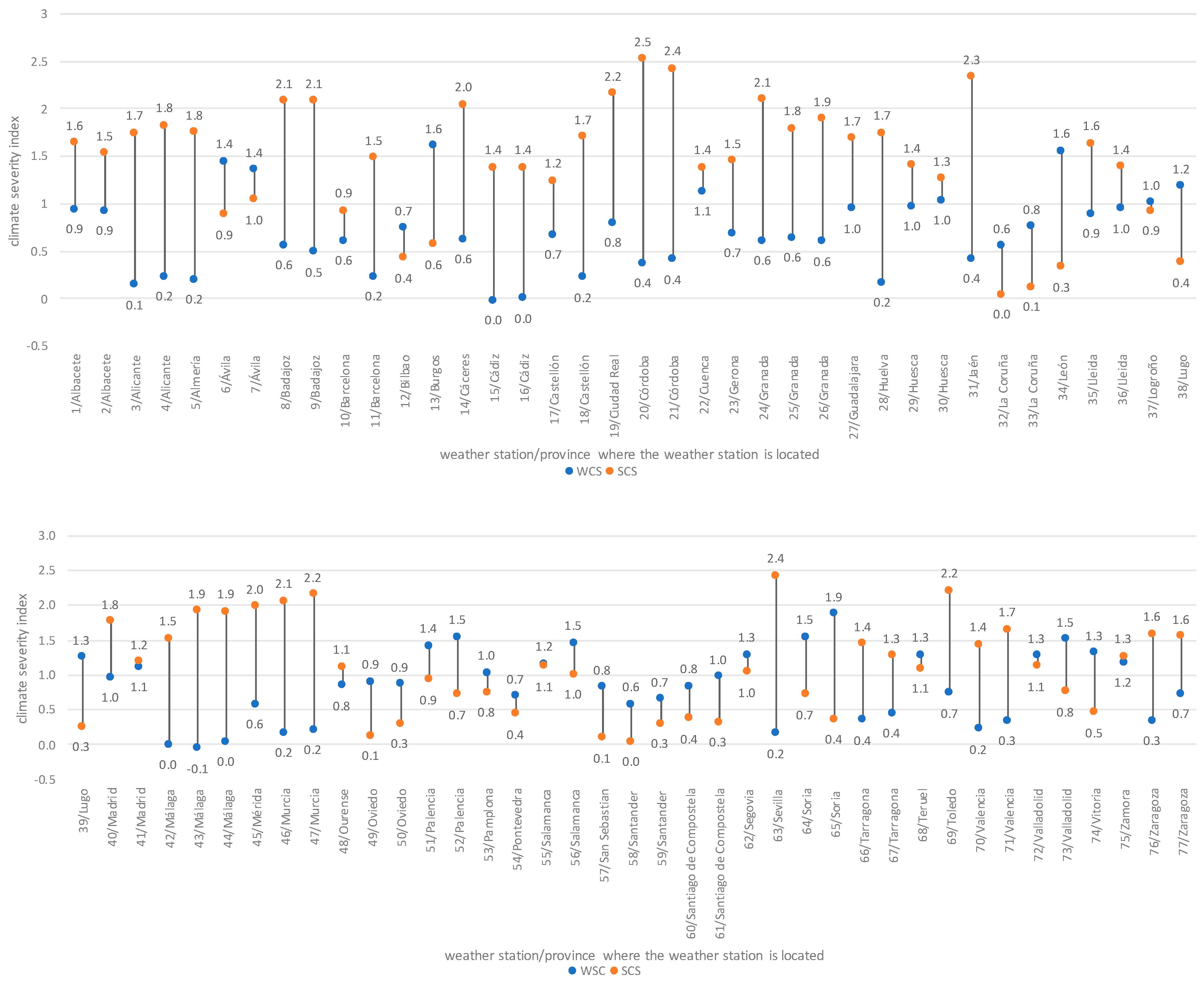
3.1. Determination of Climate Severity Indices
3.2. Determination of the Dynamics of Changes in Climate Severity Indices
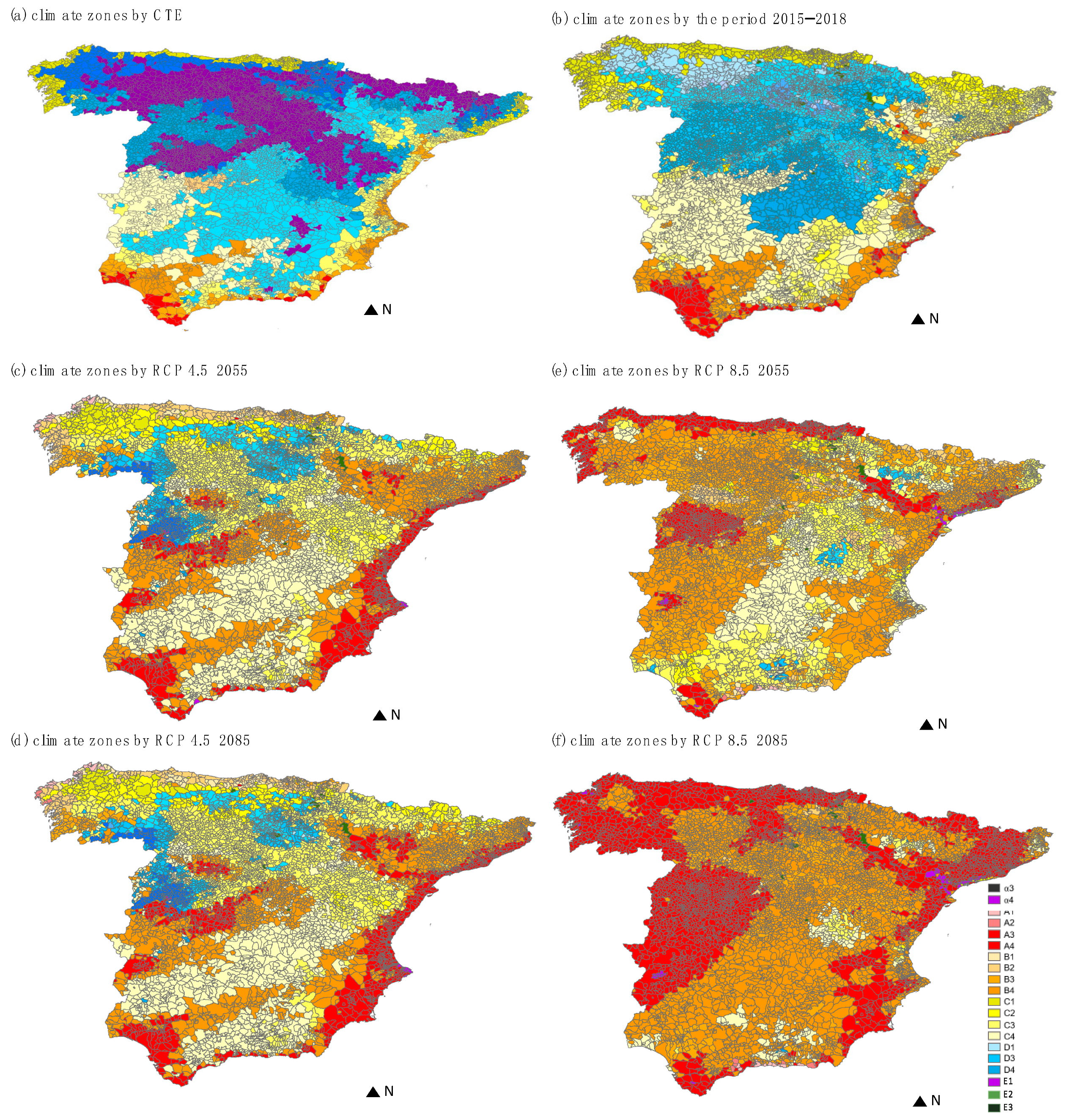
3.3. Proposed Update of Climate Zones for Peninsular Spain
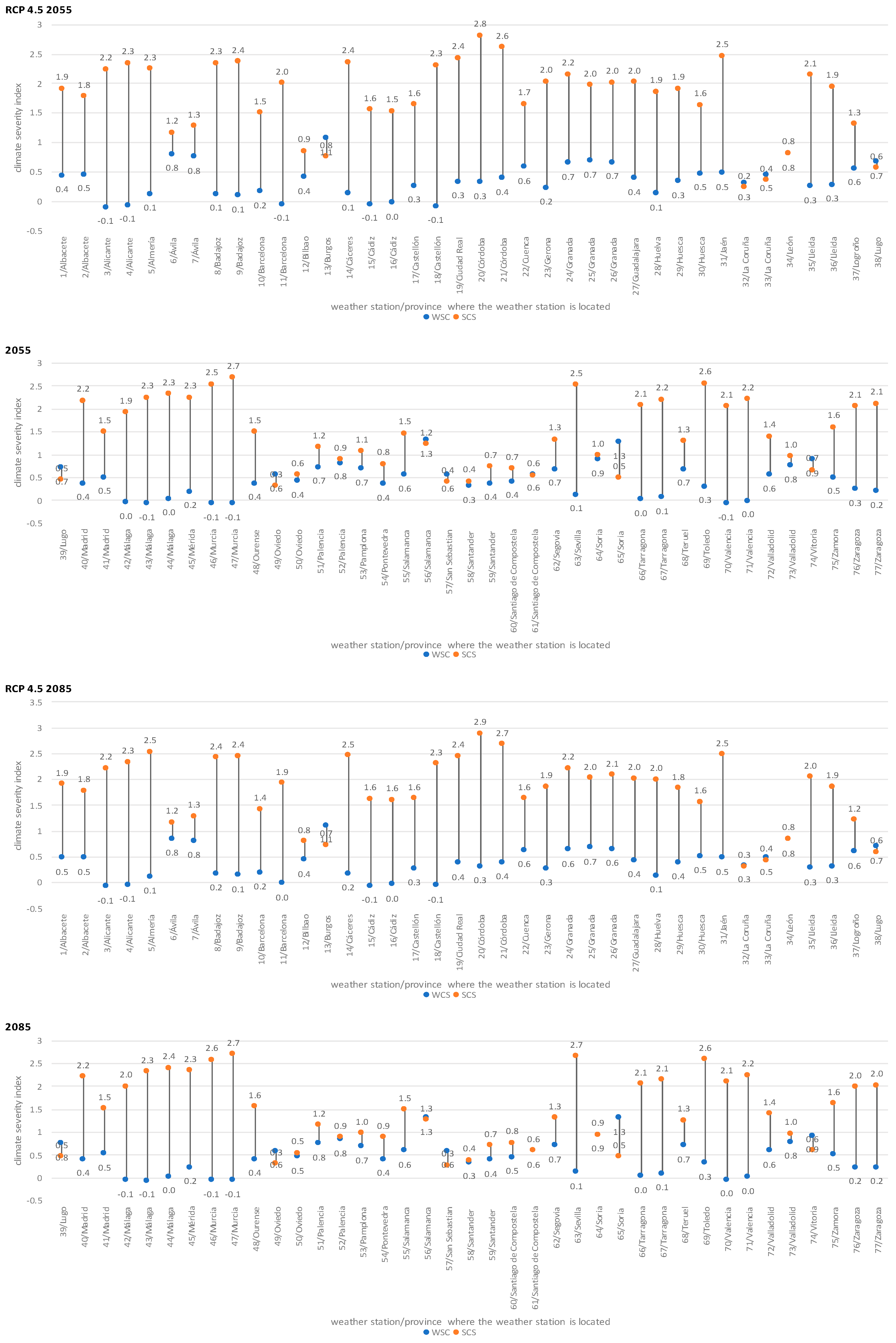
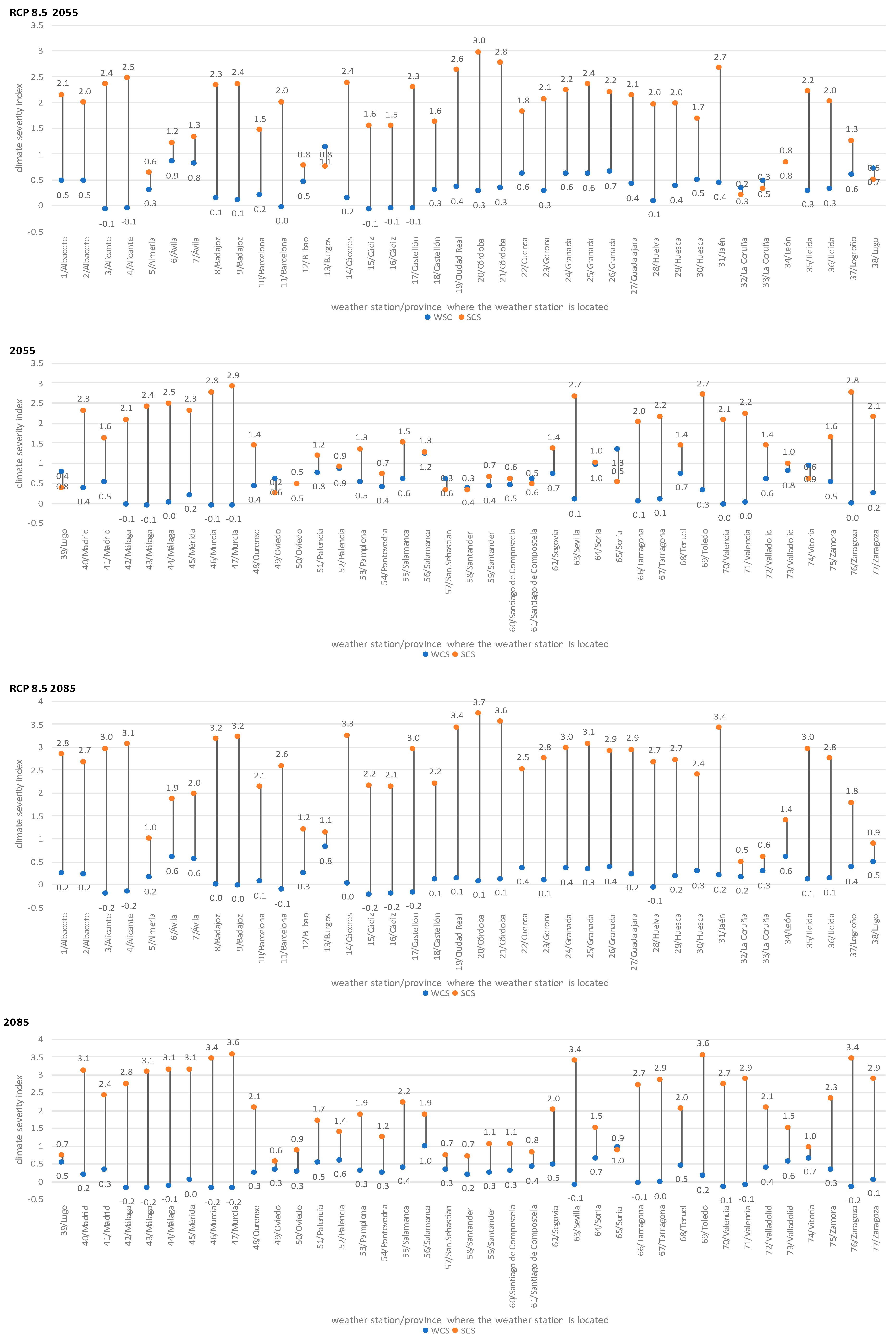
3.3.1. Climate Severities for 2015–2018 and the Periods 2055 and 2085 of the RCP 4.5 and 8.5 Scenarios for 7967 Locations in Mainland Spain
3.3.2. Proposed Update of Climate Zones for Peninsular Spain
Proposed Update of Climate Zones for Peninsular Spain for the Period 2015–2018
Proposed Climate Zones for Peninsular Spain for the RCP 4.5 Scenario Projections
Proposed Climate Zones for Peninsular Spain for the RCP 8.5 Scenario Projections
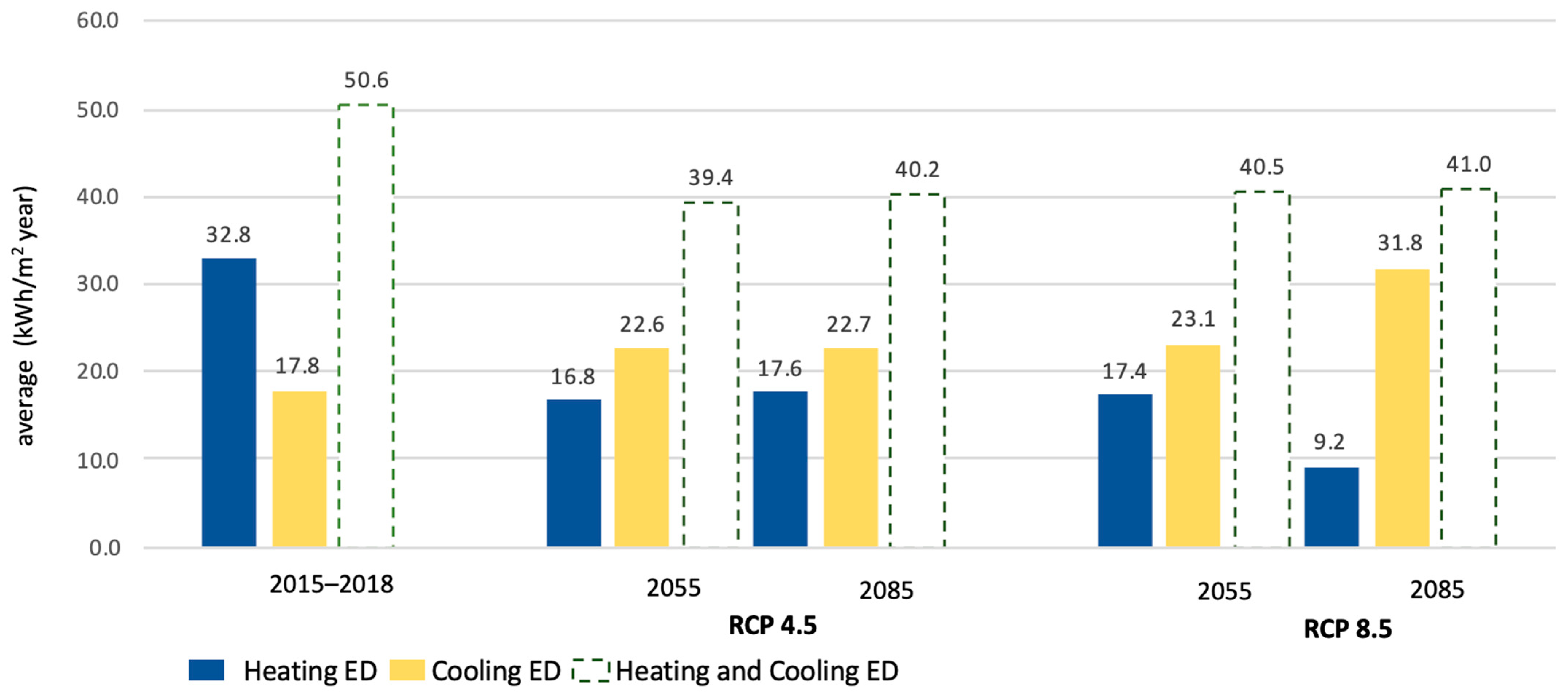
3.4. Analysis of the Dynamics of Dhanges in Energy Demand for RCP 4.5 and RCP 8.5 Scenarios
4. Conclusions
Author Contributions
Funding
Institutional Review Board Statement
Informed Consent Statement
Data Availability Statement
Conflicts of Interest
Abbreviations
| AdapteCCa | Climate Change Adaptation Platform |
| AEMET | State Meteorological Agency |
| C | cooling energy demand |
| CDD | cooling degree-days |
| CSI | climatic severity index |
| CTE | Technical Building Code |
| CZ | climate zone |
| DB-HE | Basic Document on Energy Saving |
| EC | energy consumption |
| ED | energy demand |
| ESRL | Earth System Research Laboratory |
| GDP | Gross Domestic Product |
| H | heating energy demand |
| HDD | heating degree-days |
| IPCC | Intergovernmental Panel on Climate Change |
| LLGHG | long-lived greenhouse gas emissions |
| RBF | radial basis functions |
| RF | Radiative Forcing |
| RCP | Representative Concentration Pathways |
| SCS | severity index for summer |
| WCS | severity index for winter |
| WS | Weather station |
References
- IPCC. Climate Change 2014: Synthesis Report. Contribution of Working Groups I, II and III to the Fifth Assessment Report of the Intergovernmental Panel on Climate Change; Core Writing Team, Pachauri, R.K., Meyer, L.A., Eds.; IPCC: Geneva, Switzerland, 2014; 151p. [Google Scholar]
- Houghton, J.T.; Ding, Y.D.J.G.; Griggs, D.J.; Noguer, M.; van der Linden, P.J.; Dai, X.; Johnson, C.A. Climate Change 2001: The Scientific Basis; The Press Syndicate of the University of Cambridge: Cambridge, UK, 2001; p. 881. [Google Scholar] [CrossRef]
- Chuwah, C.; Van Noije, T.; Van Vuuren, D.P.; Hazeleger, W.; Strunk, A.; Deetman, S.; Beltran, A.M.; Van Vliet, J. Implications of Alternative Assumptions Regarding Future Air Pollution Control in Scenarios Similar to the Representative Concentration Pathways. Atmos. Environ. 2013, 79, 787–801. [Google Scholar] [CrossRef]
- Verichev, K.; Zamorano, M.; Carpio, M. Effects of Climate Change on Variations in Climatic Zones and Heating Energy Consumption of Residential Buildings in the Southern Chile. Energy Build. 2020, 215, 109874. [Google Scholar] [CrossRef]
- Thomson, A.M.; Calvin, K.V.; Smith, S.J.; Kyle, G.P.; Volke, A.; Patel, P.; Delgado-Arias, S.; Bond-Lamberty, B.; Wise, M.A.; Clarke, L.E.; et al. RCP 4.5: A Pathway for Stabilization of Radiative Forcing by 2100. Clim. Chang. 2011, 109, 77–94. [Google Scholar] [CrossRef]
- Riahi, K.; Rao, S.; Krey, V.; Cho, C.; Chirkov, V.; Fischer, G.; Kindermann, G.; Nakicenovic, N.; Rafaj, P. RCP 8.5—A Scenario of Comparatively High Greenhouse gas Emissions. Clim. Chang. 2011, 109, 33–57. [Google Scholar] [CrossRef]
- Lorusso, A.; Maraziti, F. Heating System Projects Using the Degree-Days Method in Livestock Buildings. J. Agric. Eng. Res. 1998, 71, 285–290. [Google Scholar] [CrossRef]
- Troup, L.; Eckelman, M.J.; Fannon, D. Simulating Future Energy Consumption in Office Buildings Using an Ensemble of Morphed Climate Data. Appl. Energy 2019, 255, 113821. [Google Scholar] [CrossRef]
- Bellia, L.; Mazzei, P.; Palombo, A. Weather Data for Building Energy Cost-Benefit Analysis. Int. J. Energy Res. 1998, 22, 1205–1215. [Google Scholar] [CrossRef]
- Grøntoft, T. Climate Change Impact on Building Surfaces and Façades. Int. J. Clim. Chang. Strat. Manag. 2011, 3, 374–385. [Google Scholar] [CrossRef]
- Nik, V.M.; Mundt-Petersen, S.; Kalagasidis, A.S.; De Wilde, P. Future Moisture Loads for Building Facades in Sweden: Climate Change and Wind-Driven Rain. Build. Environ. 2015, 93, 362–375. [Google Scholar] [CrossRef]
- Brown, M.A.; Cox, M.; Staver, B.; Baer, P. Modeling climate-driven changes in U.S. buildings energy demand. Clim. Chang. 2016, 134, 29–44. [Google Scholar] [CrossRef]
- Christenson, M.; Manz, H.; Gyalistras, D. Climate warming impact on degree-days and building energy demand in Switzerland. Energy Convers. Manag. 2006, 47, 671–686. [Google Scholar] [CrossRef]
- De Rosa, M.; Bianco, V.; Scarpa, F.; Tagliafico, L.A. Heating and cooling building energy demand evaluation; a simplified model and a modified degree days approach. Appl. Energy 2014, 128, 217–229. [Google Scholar] [CrossRef]
- Dolinar, M.; Vidrih, B.; Kajfež-Bogataj, L.; Medved, S. Predicted changes in energy demands for heating and cooling due to climate change. Phys. Chem. Earth Parts A/B/C 2010, 35, 100–106. [Google Scholar] [CrossRef]
- Jylhä, K.; Jokisalo, J.; Ruosteenoja, K.; Pilli-Sihvola, K.; Kalamees, T.; Seitola, T.; Mäkelä, H.M.; Hyvönen, R.; Laapas, M.; Drebs, A. Energy demand for the heating and cooling of residential houses in Finland in a changing climate. Energy Build. 2015, 99, 104–116. [Google Scholar] [CrossRef]
- Berardi, U.; Jafarpur, P. Assessing the impact of climate change on building heating and cooling energy demand in Canada. Renew. Sustain. Energy Rev. 2020, 121, 109681. [Google Scholar] [CrossRef]
- da Guarda, E.L.A.; Domingos, R.M.A.; Jorge, S.H.M.; Durante, L.C.; Sanches, J.C.M.; Leão, M.; Callejas, I.J.A. The influence of climate change on renewable energy systems designed to achieve zero energy buildings in the present: A case study in the Brazilian Savannah. Sustain. Cities Soc. 2020, 52, 101843. [Google Scholar] [CrossRef]
- Hekkenberg, M.; Moll, H.; Uiterkamp, A.S. Dynamic temperature dependence patterns in future energy demand models in the context of climate change. Energy 2009, 34, 1797–1806. [Google Scholar] [CrossRef]
- Seljom, P.; Rosenberg, E.; Fidje, A.; Haugen, J.E.; Meir, M.; Rekstad, J.; Jarlset, T. Modelling the effects of climate change on the energy system—A case study of Norway. Energy Policy 2011, 39, 7310–7321. [Google Scholar] [CrossRef]
- Belzer, D.B.; Scott, M.J.; Sands, R.D. Climate Change Impacts on U.S. Commercial Building Energy Consumption: An Analysis Using Sample Survey Data. Energy Sources 1996, 18, 177–201. [Google Scholar] [CrossRef]
- Amato, A.D.; Ruth, M.; Kirshen, P.; Horwitz, J. Regional Energy Demand Responses to Climate Change: Methodology and Application to the Commonwealth of Massachusetts. Clim. Chang. 2005, 71, 175–201. [Google Scholar] [CrossRef]
- Xu, P.; Huang, Y.J.; Miller, N.; Schlegel, N.; Shen, P. Impacts of climate change on building heating and cooling energy patterns in California. Energy 2012, 44, 792–804. [Google Scholar] [CrossRef]
- Asimakopoulos, D.; Santamouris, M.; Farrou, I.; Laskari, M.; Saliari, M.; Zanis, G.; Giannakidis, G.; Tigas, K.; Kapsomenakis, J.; Douvis, C.; et al. Modelling the Energy Demand Projection of the Building Sector in Greece in the 21st Century. Energy Build. 2012, 49, 488–498. [Google Scholar] [CrossRef]
- Olonscheck, M.; Holsten, A.; Kropp, J.P. Heating and Cooling Energy Demand and Related Emissions of the German Residential Building Stock under Climate Change. Energy Policy 2011, 39, 4795–4806. [Google Scholar] [CrossRef]
- Zhai, Z.J.; Helman, J.M. Implications of Climate Changes to Building Energy and Design. Sustain. Cities Soc. 2019, 44, 511–519. [Google Scholar] [CrossRef]
- Shi, Y.; Wang, G. Changes in Building Climate Zones over China Based on High-Resolution Regional Climate Projections. Environ. Res. Lett. 2020, 15, 114045. [Google Scholar] [CrossRef]
- Belcher, S.; Hacker, J.; Powell, D. Constructing Design Weather Data for Future Climates. Build. Serv. Eng. Res. Technol. 2005, 26, 49–61. [Google Scholar] [CrossRef]
- Dodoo, A.; Gustavsson, L.; Bonakdar, F. Effects of Future Climate Change Scenarios on Overheating Risk and Primary Energy Use for Swedish Residential Buildings. Energy Procedia 2014, 61, 1179–1182. [Google Scholar] [CrossRef]
- Roux, C.; Schalbart, P.; Assoumou, E.; Peuportier, B. Integrating Climate Change and Energy Mix Scenarios in Lca Of Buildings and Districts. Appl. Energy 2016, 184, 619–629. [Google Scholar] [CrossRef]
- Sailor, D.J. Risks of Summertime Extreme Thermal Conditions in Buildings as a Result of Climate Change and Exacerbation of Urban Heat Islands. Build. Environ. 2014, 78, 81–88. [Google Scholar] [CrossRef]
- Guan, L. Preparation of Future Weather Data to Study the Impact of Climate Change on Buildings. Build. Environ. 2009, 44, 793–800. [Google Scholar] [CrossRef]
- Wang, X.; Chen, D.; Ren, Z. Assessment of Climate Change Impact on Residential Building Heating and Cooling Energy Requirement in Australia. Build. Environ. 2010, 45, 1663–1682. [Google Scholar] [CrossRef]
- Andrić, I.; Gomes, N.; Pina, A.; Ferrão, P.; Fournier, J.; Lacarrière, B.; Le Corre, O. Modeling the Long-Term Effect Of Climate Change on Building Heat Demand: Case Study on a District Level. Energy Build. 2016, 126, 77–93. [Google Scholar] [CrossRef]
- EUR-Lex-32018L0844-EN-EUR-Lex. Available online: https://eur-lex.europa.eu/eli/dir/2018/844/oj (accessed on 15 April 2020).
- Mulvaney, D. Green New Deal. Solar Power 2019, 47–65. [Google Scholar] [CrossRef]
- Australian Building Codes Board. Handbook: Energy Efficiency NCC Volume Two. 2019. Available online: https://www.abcb.gov.au/Resources/Publications/Education-Training/energy-efficiency-ncc-volume-two (accessed on 14 January 2021).
- International Code Council. The International Energy Conservation Code (IECC). 2000. Available online: https://shop.iccsafe.org/2000-international-energy-conservation-coder-pdf-download.html (accessed on 22 December 2020).
- HULC Unified Tool LIDER-CALENER, Version 1.0.1493.1049 (Herramienta Unificada LIDER-CALENER, Versión 1.0.1493.1049). Available online: http://www.codigotecnico.org/index.php/menu-recursos/menu-aplicaciones/282-herramienta-unificada-lider-calener (accessed on 1 July 2016).
- Rakoto-Joseph, O.; Garde, F.; David, M.; Adelard, L.; Randriamanantany, Z. Development of Climatic Zones and Passive Solar Design in Madagascar. Energy Convers. Manag. 2009, 50, 1004–1010. [Google Scholar] [CrossRef]
- Walsh, A.; Cóstola, D.; Labaki, L.C. Review of Methods for Climatic Zoning for Building Energy Efficiency Programs. Build. Environ. 2017, 112, 337–350. [Google Scholar] [CrossRef]
- Ministerio de Fomento Documento Básico HE Ahorro de Energía 2019. Código Técnico de la Edificacion 2019, 1–129.
- Ferreira, M.; Coelho, M.J.P.; Alves, R.V.L. Regulamento das Características de Comportamento Térmico de Edifícios (RCCTE): Desenvolvimento de Folha de Cálculo; Edições Universidade Fernando Pessoa: Porto, Portugal, 2009; pp. 67–75. [Google Scholar]
- France. Code de La Construction et de l’ Habitation Partie Législative Livre Ier: Dispositions Générales. Titre Préliminaire: Informations Du Parlement En Matière de Logement Partie Législative Livre Ier: Dispositions Générales. Titre Ier Constr. Des. 2011, 2007–2008.
- Carpio, M.; Jódar, J.; Rodíguez, M.L.; Zamorano, M. A Proposed Method Based on Approximation and Interpolation for Determining Climatic Zones and Its Effect on Energy Demand and CO2 Emissions from Buildings. Energy Build. 2015, 87, 253–264. [Google Scholar] [CrossRef]
- Lastra-Bravo, X.B.; Fernández-Membrive, V.J.; Flores-Parra, I.; Tolón-Becerra, A. Energy Qualification in Buildings. The Effect of Changes in Construction Methods in the Spanish A4 Climate Zone. Energy Procedia 2013, 42, 513–522. [Google Scholar] [CrossRef]
- Salmerón, J.; Álvarez, S.; Molina, J.; Ruiz, A.; Sánchez, F. Tightening the Energy Consumptions of Buildings Depending on Their Typology and on Climate Severity Indexes. Energy Build. 2013, 58, 372–377. [Google Scholar] [CrossRef]
- State Meteorological Agency-AEMET-Spanish Government. Available online: http://www.aemet.es/es/portada (accessed on 15 April 2021).
- NOAA ESRL GMD NOAA Solar Calculation. Available online: https://www.esrl.noaa.gov/gmd/grad/solcalc/calcdetails.html (accessed on 20 January 2021).
- National Platform for Adaptation to Climate Change. Available online: https://www.adaptecca.es/en (accessed on 20 January 2021).
- Jiang, A.; Zhu, Y.; Elsafty, A.; Tumeo, M. Effects of Global Climate Change on Building Energy Consumption and Its Implications in Florida. Int. J. Constr. Educ. Res. 2018, 14, 22–45. [Google Scholar] [CrossRef]
- Chan, A. Developing Future Hourly Weather Files for Studying the Impact of Climate Change on Building Energy Performance in Hong Kong. Energy Build. 2011, 43, 2860–2868. [Google Scholar] [CrossRef]
- Burden, R.L.; Faires, J.D.; Burden, A.M. Numerical Analysis; Cengage: New York, NY, USA, 2016; ISBN 9781305253667. [Google Scholar]
- Buhmann, M.D. Radial basis functions. Acta Numer. 2000, 9, 1–38. [Google Scholar] [CrossRef]
- López-Ochoa, L.M.; Las-Heras-Casas, J.; López-González, L.M.; García-Lozano, C. Environmental and Energy Impact of the Epbd in Residential Buildings in Cold Mediterranean Zones: The Case of Spain. Energy Build. 2017, 150, 567–582. [Google Scholar] [CrossRef]
- Royal Decree 314/2006 of March 17, Approving the Technical Building Code (Real Decreto 314/2006, de 17 de Marzo, Por El Que Se Aprueba El Código Técnico de La Edificación). Available online: http://www.boe.es/boe/dias/2006/03/28/pdfs/A11816-11831.pdf (accessed on 20 July 2020).
- Avendaño-Vera, C.; Martinez-Soto, A.; Marincioni, V. Determination of Optimal Thermal Inertia of Building Materials for Housing in Different Chilean Climate Zones. Renew. Sustain. Energy Rev. 2020, 131, 110031. [Google Scholar] [CrossRef]
- Parker, J. The Leeds Urban Heat Island and Its Implications for Energy Use and Thermal Comfort. Energy Build. 2021, 235, 110636. [Google Scholar] [CrossRef]
- Adloff, F.; Somot, S.; Sevault, F.; Jordà, G.; Aznar, R.; Déqué, M.; Herrmann, M.; Marcos, M.; Dubois, C.; Padorno, E.; et al. Mediterranean Sea Response to Climate Change in an Ensemble of Twenty First Century Scenarios. Clim. Dyn. 2015, 45, 2775–2802. [Google Scholar] [CrossRef]


| Intervals for Winter Zoning | |||||
| α | A | B | C | D | E |
| WCS ≤ 0 | 0 < WCS ≤ 0.23 | 0.23 < WCS ≤ 0.5 | 0.5 < WCS ≤ 0.93 | 0.93 < WCS ≤ 1.51 | WCS > 1.51 |
| Intervals for Summer Zoning | |||||
| 1 | 2 | 3 | 4 | ||
| SCS ≤ 0.5 | 0.5 < SCS ≤ 0.83 | 0.83 < SCS ≤ 1.38 | SCS > 1.38 | ||
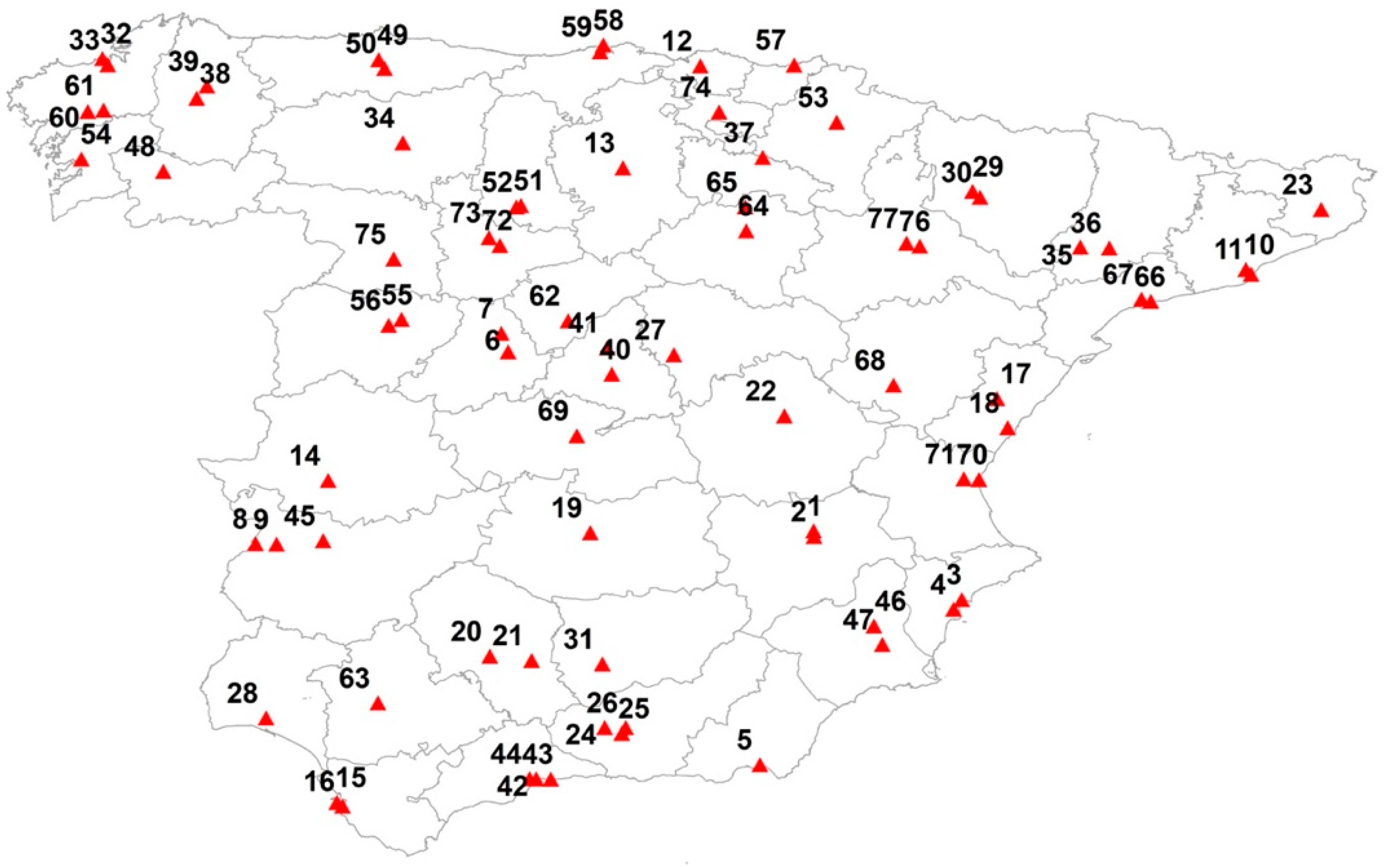
| WS | Latitude | Longitude | Altitude | WCS | SCS | WS | Latitude | Longitude | Altitude | WCS | SCS |
|---|---|---|---|---|---|---|---|---|---|---|---|
| 1 | 39.00556 | −1.862222 | 676 | 0.94 | 1.64 | 40 | 40.45167 | −3.724167 | 664 | 0.96 | 1.76 |
| 2 | 38.95417 | −1.856389 | 702 | 0.92 | 1.53 | 41 | 40.69611 | −3.765000 | 1004 | 1.11 | 1.19 |
| 3 | 38.37250 | −0.494167 | 22 | 0.14 | 1.74 | 42 | 36.71667 | −4.419722 | 25 | −0.01 | 1.52 |
| 4 | 38.28278 | −0.570833 | 43 | 0.23 | 1.82 | 43 | 36.71500 | −4.286111 | 7 | −0.06 | 1.91 |
| 5 | 36.84691 | −2.356989 | 21 | 0.20 | 1.75 | 44 | 36.71778 | −4.481667 | 54 | 0.04 | 1.90 |
| 6 | 40.65917 | −4.680000 | 1130 | 1.44 | 0.88 | 45 | 38.91583 | −6.385556 | 228 | 0.57 | 1.98 |
| 7 | 40.82889 | −4.741944 | 920 | 1.36 | 1.04 | 46 | 38.12806 | −1.305833 | 150 | 0.17 | 2.05 |
| 8 | 38.88750 | −7.008056 | 175 | 0.56 | 2.08 | 47 | 37.95778 | −1.228611 | 75 | 0.21 | 2.15 |
| 9 | 38.88333 | −6.813889 | 185 | 0.49 | 2.08 | 48 | 42.32528 | −7.859722 | 442 | 0.84 | 1.11 |
| 10 | 41.41833 | 2.124167 | 408 | 0.61 | 0.92 | 49 | 43.35333 | −5.874167 | 336 | 0.90 | 0.12 |
| 11 | 41.37500 | 2.173889 | 5 | 0.23 | 1.48 | 50 | 43.27500 | −5.819167 | 170 | 0.86 | 0.29 |
| 12 | 43.29806 | −2.906389 | 42 | 0.74 | 0.43 | 51 | 42.00944 | −4.560556 | 736 | 1.41 | 0.93 |
| 13 | 42.35694 | −3.620278 | 891 | 1.61 | 0.57 | 52 | 41.99556 | −4.602778 | 874 | 1.54 | 0.71 |
| 14 | 39.47139 | −6.338889 | 10 | 0.62 | 2.04 | 53 | 42.77750 | −1.649722 | 459 | 1.02 | 0.75 |
| 15 | 36.49972 | −6.257778 | 2 | −0.02 | 1.38 | 54 | 42.43833 | −8.615833 | 108 | 0.69 | 0.43 |
| 16 | 36.46556 | −6.205556 | 28 | 0.00 | 1.380 | 55 | 40.95750 | −5.662222 | 775 | 1.15 | 1.12 |
| 17 | 40.22722 | −0.169722 | 10 | 0.67 | 1.24 | 56 | 40.90361 | −5.779722 | 817 | 1.45 | 1.00 |
| 18 | 39.95722 | −0.071944 | 43 | 0.22 | 1.70 | 57 | 43.30639 | −2.041111 | 251 | 0.82 | 0.09 |
| 19 | 38.98917 | −3.920278 | 628 | 0.80 | 2.16 | 58 | 43.49111 | −3.800556 | 52 | 0.57 | 0.04 |
| 20 | 37.84889 | −4.846667 | 90 | 0.37 | 2.52 | 59 | 43.42861 | −3.831389 | 3 | 0.65 | 0.30 |
| 21 | 37.81028 | −4.462222 | 275 | 0.41 | 2.42 | 60 | 42.87611 | −8.555833 | 240 | 0.83 | 0.37 |
| 22 | 40.06722 | −2.131944 | 948 | 1.13 | 1.38 | 61 | 42.88806 | −8.410556 | 370 | 0.97 | 0.32 |
| 23 | 41.97222 | 2.819444 | 76 | 0.69 | 1.45 | 62 | 40.94528 | −4.126389 | 1005 | 1.28 | 1.04 |
| 24 | 37.18972 | −3.789444 | 567 | 0.61 | 2.10 | 63 | 37.41667 | −5.879167 | 34 | 0.16 | 2.420 |
| 25 | 37.13722 | −3.631389 | 687 | 0.64 | 1.79 | 64 | 41.77500 | −2.483056 | 1082 | 1.54 | 0.710 |
| 26 | 37.18972 | −3.595556 | 775 | 0.60 | 1.89 | 65 | 41.99583 | −2.494167 | 1260 | 1.87 | 0.360 |
| 27 | 40.63028 | −3.150000 | 721 | 0.95 | 1.69 | 66 | 41.12389 | 1.249167 | 55 | 0.35 | 1.440 |
| 28 | 37.27833 | −6.911667 | 19 | 0.17 | 1.74 | 67 | 41.14500 | 1.163611 | 71 | 0.44 | 1.270 |
| 29 | 42.13889 | −0.395000 | 463 | 0.97 | 1.40 | 68 | 40.35056 | −1.124167 | 900 | 1.28 | 1.090 |
| 30 | 42.08444 | −0.325556 | 546 | 1.03 | 1.26 | 69 | 39.88472 | −4.045278 | 515 | 0.74 | 2.200 |
| 31 | 37.77750 | −3.808889 | 580 | 0.42 | 2.33 | 70 | 39.47972 | −0.337500 | 6 | 0.22 | 1.430 |
| 32 | 43.36583 | −8.421389 | 58 | 0.55 | 0.04 | 71 | 39.48500 | −0.474722 | 56 | 0.34 | 1.650 |
| 33 | 43.30694 | −8.371944 | 98 | 0.76 | 0.12 | 72 | 41.64083 | −4.754444 | 735 | 1.27 | 1.120 |
| 34 | 42.58833 | −5.651111 | 912 | 1.55 | 0.33 | 73 | 41.71194 | −4.855556 | 846 | 1.51 | 0.760 |
| 35 | 41.62611 | 0.598056 | 185 | 0.89 | 1.63 | 74 | 42.87194 | −2.732778 | 513 | 1.32 | 0.460 |
| 36 | 41.61694 | 0.866667 | 252 | 0.95 | 1.39 | 75 | 41.51556 | −5.735278 | 656 | 1.18 | 1.260 |
| 37 | 42.45222 | −2.331111 | 353 | 1.01 | 0.92 | 76 | 41.63333 | −0.882222 | 258 | 0.34 | 1.580 |
| 38 | 42.99833 | −7.552500 | 442 | 1.18 | 0.38 | 77 | 41.66056 | −1.004167 | 249 | 0.72 | 1.550 |
| 39 | 43.11139 | −7.457500 | 445 | 1.25 | 0.25 |
| Scenario | Winter Climatic Zone | Summer Climatic Zone | Winter + Summer Climatic Zone | ||||
|---|---|---|---|---|---|---|---|
| Code Number of CZ that Change | % of Cities Modifying CZ | % of Cities that Change CZ | Code Number of CZ that Change | % of Cities Modifying CZ | % of Cities that Change CZ | % of Cities that Change CZ | |
| 2015–2018 | 1 | 47.2% | 52.1% | 1 | 58.7% | 72.0% | 84% |
| 2 | 4.4% | 2 | 12.2% | ||||
| 3 | 0.1% | 3 | 0.2% | ||||
| 4 | 0.1% | 4 | 0.0% | ||||
| 5 | 0.1% | −1 | 0.9% | ||||
| −1 | 0.1% | ||||||
| RCP 4.5 2055 | 1 | 44.8% | 89.0% | 1 | 47.7% | 88.6% | 98% |
| 2 | 40.5% | 2 | 39.4% | ||||
| 3 | 3.0% | 3 | 1.4% | ||||
| 4 | 0.0% | 4 | 0.0% | ||||
| 5 | 0.0% | −1 | 0.1% | ||||
| −1 | 0.7% | ||||||
| RCP 4.5 2085 | 1 | 41.0% | 89.9% | 1 | 48.3% | 87.6% | 98% |
| 2 | 43.4% | 2 | 38.1% | ||||
| 3 | 4.7% | 3 | 1.2% | ||||
| 4 | 0.1% | 4 | 0.0% | ||||
| 5 | 0.0% | −1 | 0.1% | ||||
| −1 | 0.7% | ||||||
| RCP 8.5 2055 | 1 | 24.4% | 92.4% | 1 | 33.0% | 82.7% | 97% |
| 2 | 33.1% | 2 | 25.5% | ||||
| 3 | 26.5% | 3 | 18.9% | ||||
| 4 | 4.1% | 4 | 0.0% | ||||
| 5 | 0.0% | −1 | 4.1% | ||||
| −1 | 3.8% | ||||||
| RCP 8.5 2085 | 1 | 10.1% | 100% | 1 | 31.0% | 91.0% | 98% |
| 2 | 36.7% | 2 | 26.3% | ||||
| 3 | 35.4% | 3 | 32.2% | ||||
| 4 | 11.6% | 4 | 0.0% | ||||
| 5 | 0.0% | −1 | 1.1% | ||||
| −1 | 0.6% | ||||||
| Climatic Zone | Present | RCP 4.5 | RCP 8.5 | |||
|---|---|---|---|---|---|---|
| CTE | 2015–2018 | 2055 | 2085 | 2055 | 2085 | |
| Winter Climatic Zone | ||||||
| α | 0.00% | 0.02% | 0.15% | 0.25% | 0.41% | 0.70% |
| A | 0.74% | 2.85% | 12.89% | 15.97% | 16.62% | 42.95% |
| B | 5.47% | 8.39% | 29.21% | 28.28% | 53.39% | 51.54% |
| C | 20.05% | 37.18% | 43.54% | 43.03% | 28.28% | 4.63% |
| D | 44.90% | 49.13% | 11.60% | 9.84% | 1.27% | 0.16% |
| E | 28.76% | 2.41% | 2.59% | 2.60% | 0.01% | 0.00% |
| Summer Climatic Zone | ||||||
| 1 | 40.05% | 8.65% | 1.41% | 2.11% | 0.99% | 0.38% |
| 2 | 22.80% | 23.79% | 10.53% | 11.83% | 8.11% | 0.44% |
| 3 | 28.58% | 38.21% | 38.54% | 36.45% | 41.02% | 13.83% |
| 4 | 8.55% | 29.35% | 49.51% | 49.60% | 49.84% | 85.31% |
| Climatic Zone (Winter + Summer) | ||||||
| α3 | 0.00% | 0.01% | 0.00% | 0.00% | 0.00% | 0.00% |
| α4 | 0.00% | 0.01% | 0.15% | 0.25% | 0.41% | 0.70% |
| A1 | 0.00% | 0.00% | 0.19% | 0.23% | 0.11% | 0.18% |
| A2 | 0.00% | 0.00% | 0.04% | 0.08% | 0.01% | 0.13% |
| A3 | 0.40% | 0.13% | 0.03% | 0.14% | 0.92% | 2.82% |
| A4 | 0.34% | 2.72% | 12.64% | 15.53% | 15.54% | 39.74% |
| B1 | 0.00% | 0.19% | 0.58% | 1.04% | 0.33% | 0.04% |
| B2 | 0.00% | 0.03% | 3.00% | 3.09% | 5.35% | 0.21% |
| B3 | 3.08% | 0.65% | 4.04% | 4.31% | 22.38% | 9.62% |
| B4 | 2.40% | 7.52% | 21.57% | 19.82% | 25.26% | 41.63% |
| C1 | 2.87% | 5.57% | 0.62% | 0.77% | 0.41% | 0.11% |
| C2 | 3.21% | 3.80% | 4.10% | 4.86% | 2.45% | 0.10% |
| C3 | 8.15% | 13.93% | 23.80% | 23.89% | 16.88% | 1.37% |
| C4 | 5.81% | 13.85% | 14.90% | 13.41% | 8.50% | 3.05% |
| D1 | 8.21% | 2.42% | 0.03% | 0.08% | 0.13% | 0.05% |
| D2 | 19.58% | 17.81% | 3.26% | 3.68% | 0.30% | 0.00% |
| D3 | 16.96% | 23.49% | 8.06% | 5.51% | 0.80% | 0.03% |
| D4 | 0.00% | 5.26% | 0.25% | 0.58% | 0.04% | 0.09% |
| E1 | 28.76% | 0.39% | 0.00% | 0.00% | 0.01% | 0.00% |
| E2 | 0.00% | 2.01% | 0.05% | 0.04% | 0.00% | 0.00% |
| E3 | 0.00% | 0.01% | 2.54% | 2.55% | 0.00% | 0.00% |
| 2015–2018 | RCP 4.5 | ||||||||||||
| 2055 | Change | 2085 | Change | ||||||||||
| ED between 2015–2018 and 2055 | ED between 2015–2018 and 2085 | ||||||||||||
| ED | ED | ED | |||||||||||
| H | C | H + C | H | C | H + C | H | C | H | C | H + C | H | C | |
| 73 | 64.5 | 10.7 | 75.2 | 32.5 | 13.5 | 46.0 | 32.1 | −2.8 | 33.8 | 13.5 | 47.3 | 30.8 | −2.8 |
| 5 | 8.5 | 24.7 | 33.2 | 5.1 | 31.7 | 36.8 | 3.4 | −7.0 | 4.7 | 35.5 | 40.2 | 3.8 | −10.8 |
| 17 | 28.6 | 17.5 | 46.1 | 11.1 | 23.1 | 34.2 | 17.5 | −5.6 | 11.5 | 22.8 | 34.4 | 17.1 | −5.4 |
| 76 | 14.5 | 22.3 | 36.8 | 10.7 | 29.0 | 39.7 | 3.8 | −6.8 | 9.4 | 27.9 | 37.3 | 5.1 | −5.6 |
| RCP 8.5 | |||||||||||||
| 2055 | change | 2085 | change | ||||||||||
| ED | ED between 2015–2018 and 2055 | ED | ED between 2015−2018 and 2085 | ||||||||||
| H | C | H + C | H | C | H | C | H + C | H | C | ||||
| 73 | 33.8 | 13.8 | 47.6 | 30.8 | −3.1 | 23.5 | 21.4 | 44.9 | 41.0 | −10.7 | |||
| 5 | 12.8 | 8.9 | 21.7 | −4.3 | 15.8 | 6.4 | 14.1 | 20.5 | 2.1 | 10.6 | |||
| 17 | −2.1 | 32.3 | 30.1 | 30.8 | −14.8 | −7.3 | 41.6 | 34.3 | 35.9 | −24.1 | |||
| 76 | −0.9 | 39.0 | 38.2 | 15.4 | −16.8 | −6.4 | 48.5 | 42.1 | 20.9 | −26.2 | |||
Publisher’s Note: MDPI stays neutral with regard to jurisdictional claims in published maps and institutional affiliations. |
© 2021 by the authors. Licensee MDPI, Basel, Switzerland. This article is an open access article distributed under the terms and conditions of the Creative Commons Attribution (CC BY) license (https://creativecommons.org/licenses/by/4.0/).
Share and Cite
Díaz-López, C.; Jódar, J.; Verichev, K.; Rodríguez, M.L.; Carpio, M.; Zamorano, M. Dynamics of Changes in Climate Zones and Building Energy Demand. A Case Study in Spain. Appl. Sci. 2021, 11, 4261. https://doi.org/10.3390/app11094261
Díaz-López C, Jódar J, Verichev K, Rodríguez ML, Carpio M, Zamorano M. Dynamics of Changes in Climate Zones and Building Energy Demand. A Case Study in Spain. Applied Sciences. 2021; 11(9):4261. https://doi.org/10.3390/app11094261
Chicago/Turabian StyleDíaz-López, Carmen, Joaquín Jódar, Konstantin Verichev, Miguel Luis Rodríguez, Manuel Carpio, and Montserrat Zamorano. 2021. "Dynamics of Changes in Climate Zones and Building Energy Demand. A Case Study in Spain" Applied Sciences 11, no. 9: 4261. https://doi.org/10.3390/app11094261
APA StyleDíaz-López, C., Jódar, J., Verichev, K., Rodríguez, M. L., Carpio, M., & Zamorano, M. (2021). Dynamics of Changes in Climate Zones and Building Energy Demand. A Case Study in Spain. Applied Sciences, 11(9), 4261. https://doi.org/10.3390/app11094261