Article

Neuro-Inspired Computing with Spin-VCSELs

Applied Physics Research Group, Vrije Universiteit Brussel, Pleinlaan 2, 1050 Brussels, Belgium
*
Authors to whom correspondence should be addressed.
Appl. Sci. 2021, 11(9), 4232; https://doi.org/10.3390/app11094232
Submission received: 9 March 2021 / Revised: 29 April 2021 / Accepted: 1 May 2021 / Published: 7 May 2021
(This article belongs to the Special Issue Photonics for Optical Computing)

Abstract

:
Delay-based reservoir computing (RC), a neuromorphic computing technique, has gathered lots of interest, as it promises compact and high-speed RC implementations. To further boost the computing speeds, we introduce and study an RC setup based on spin-VCSELs, thereby exploiting the high polarization modulation speed inherent to these lasers. Based on numerical simulations, we benchmarked this setup against state-of-the-art delay-based RC systems and its parameter space was analyzed for optimal performance. The high modulation speed enabled us to have more virtual nodes in a shorter time interval. However, we found that at these short time scales, the delay time and feedback rate heavily influence the nonlinear dynamics. Therefore, and contrary to other laser-based RC systems, the delay time has to be optimized in order to obtain good RC performances. We achieved state-of-the-art performances on a benchmark timeseries prediction task. This spin-VCSEL-based RC system shows a ten-fold improvement in processing speed, which can further be enhanced in a straightforward way by increasing the birefringence of the VCSEL chip.

1. Introduction

Reservoir computing (RC) is a neuromorphic computing technique which is gaining popularity rapidly in our age of Big Data and Digital Sustainability, because there is an urgent need for high-speed and energy-efficient computing techniques [1]. RC employs the transient dynamics of a nonlinear reservoir to map input data unto a high dimensional state space. An output layer can be constructed by sampling from this high dimensional state space and trained to perform tasks that are notoriously difficult for CPU-based algorithmic computing approaches, such as speech and pattern recognition, system identification and timeseries prediction [2,3,4,5]. The main advantage of RC is the simplification of the training procedure, as only a single layer of nodes needs to be trained and the larger part of the network (the reservoir) is left as it is.
The reservoir of an RC system can be any dynamical system that has an accessible high dimensional state space. Typically, the reservoirs are categorized into spatially and temporally distributed reservoirs. In spatially distributed reservoirs, the individual neurons (or nodes) can be accessed individually to read out their state value, very much like neural networks. Some successful examples of spatially distributed reservoirs are echo state networks [6,7], liquid state machines [8,9], a network of memristors [10], a network of on-chip ring resonators [5,11,12] or an array of VCSELs [13]. RC with temporally distributed reservoirs is generally known as a delay-based RC system [14]. A single nonlinear dynamical system is subjected to feedback, which creates a recurrent network. The nonlinear response of the RC system is enriched by preprocessing the input data with a step-wise constant mask. The nodes in this case can be accessed indirectly by sampling the temporal stream, hence we speak of virtual nodes. Photonic systems are especially interesting to this end, because of their high-speed response and energy efficiency. Some examples of photonic delay-based reservoir computing systems are a semiconductor laser subjected to feedback with electrical data injection [15,16] or optical data injection [17,18,19,20]. Delay-based RC lends itself very well for integrated design and the first results were achieved in [21,22]. An overview of all the (photonic) RC systems can be found in [3,5,21].
Due to the time-multiplexed nodes in a delay-based RC setup, the processing speed is inversely proportional to the duration of a single sample. This duration is determined by the number of nodes and the length of these nodes in the time domain. In [17], processing speeds around 10 MSa/s could be achieved, limited by the relaxation oscillations in the intensity. Follow-up research in [18] showed that the length of the nodes could be shortened thanks to phase dynamics occurring in the system, leading to speeds of 0.25 GSa/s. In [19], it was suggested to further increase the processing speed by spreading the number of nodes over different longitudinal modes available in the laser cavity.
Recently, ultra-fast modulation techniques have been demonstrated by relying on the polarization dynamics of spin-VCSELs [23,24,25]. Modulation speeds of up to 200 GHz were achieved in [26]. We conjecture that this fast modulation speed can be used to speed up delay-based RC systems. In this work, we numerically investigated a delay-based RC system using a spin-VCSEL and injecting the data via the pump ellipticity, such that we can employ the ultra-fast polarization dynamics to increase the processing speed. Previously, there have been numerical studies on delay-based RC systems using VCSELs, but they rather rely on the phase dynamics and the polarization modes only serve to increase the state diversity in the output layer via polarization multiplexing [27,28].
In the next section, we describe the model we used for the spin-VCSEL and we provide details on our RC setup. Afterwards, we present the results obtained from different parameter scans, accompanied by a discussion, followed by the conclusions.

2. The Theoretical Model
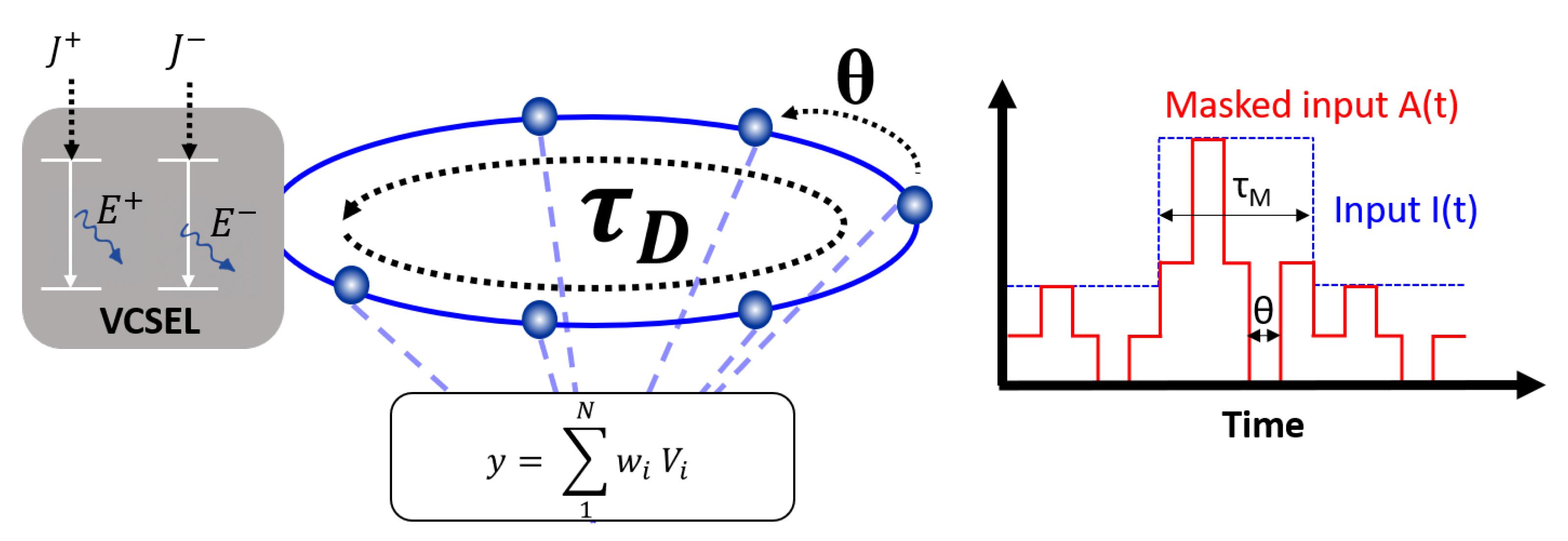
2.1. The Spin-VCSEL

The spin-flip model as described in [26] is used to simulate the spin-VCSEL, as it has been shown to correctly describe the experimentally observed behavior of these lasers. We extend the model to incorporate the optical feedback, which gives us the following rate equations:
E ˙ ± = 1 2 τ p 1 + i α N ± n 1 E ± γ a + i γ p E ϵ a + i ϵ p E ± 2 E ± + η e i Ω E ± ( t τ D )
N ˙ = γ J + ( t ) + J ( t ) N N + n E + 2 N n E 2
n ˙ = γ J + ( t ) J ( t ) N + n E + 2 + N n E 2 γ s n
Here, E ± stands for the right (+) and left (-) circularly polarized components of the slowly varying amplitudes of the electric field, N is the total population inversion in the laser with a decay rate γ and n is the population difference between the spin-up and spin-down electrons with a decay rate γ s due to spin relaxation. The photon lifetime and linewidth enhancement factor are given by, respectively, τ p and α . The amplitude and phase anisotropies of the laser cavity are given by γ a and γ p . The term ϵ a + i ϵ p E ± 2 E ± takes into account saturation effects associated with the amplitude and phase of the field. In the last term of Equation (1), E ± ( t τ D ) is the optical feedback after a delay τ D , Ω is the constant feedback phase and η is the feedback rate. J ± are the time-dependent pumping rates of spin-up (+) and spin-down (-) electrons. In practice, as mentioned in [26], the spin-VCSEL has an electrical pump J 0 and a pulsed optical spin injection. The electrical pump contributes equally to the spin-up and spin-down populations, whereas the individual populations can be pumped separately with the optical spin injection. The pumping mechanism is further explained in Section 2.2, since it is also the mechanism used to inject data.
The values used for the different parameters are summarized in Table 1. The parameters of the spin-VCSEL were chosen to be the same as in [26], where a bitstream was being modulated at speeds of 240 Gbit/s. The electrical pump and optical pump amplitude were chosen after a few exploratory trials and in Section 3.3 an extensive scan was performed to find the optimized values. The number of nodes was scanned from 5 to 100, as the typical number lies in this range [19,20,21]. The node spacing is scanned over a range from 0.5 ps to 10 ps, which is centered around the period of the polarization oscillation π γ p , because the node spacing is typically of the same order of magnitude as the fastest time scale present in the system [3,14].

2.2. The RC Setup

A schematic overview of the simulated theoretical model is shown on the left in Figure 1. A spin-VCSEL is connected to a delay line, which has a round-trip time τ D . Data are injected in the VCSEL through the optical spin injection, such that we achieve the following pump rates:
J + = J 0 2 + δ J A ( t ) and J = J 0 2 ,
where J 0 is the previously mentioned electrical pump, δ J is the amplitude of the optical spin injection and A ( t ) is the normalized masked data that is to be processed. The masked data A ( t ) are obtained via the product I ( t ) M ( t ) , where I ( t ) is the input data and M ( t ) is a sequence periodically repeating a mask. The masked data A ( t ) are normalized between 0 and 1. The mask consists of N step-wise constant levels of duration θ . Each datapoint in I ( t ) is held constant for a duration τ M = N θ that corresponds to the mask length, as shown on the right in Figure 1. The purpose of the different levels in the mask is to create diversity in the nonlinear response of the VCSEL, such that we obtain a diverse set of virtual nodes spread along the delay line. The mask length τ M is often matched to the delay time τ D , however, in this paper, this is not the case and τ M can be much larger than τ D , such that a single masked datapoint is spread over multiple roundtrips of the delay line. A principal mask is generated for a maximum of 100 nodes by randomly selecting each mask level from the following set, 0 , 0.25 , 0.5 , 0.75 , 1 . If N < 100 , we used the first N values from this principal mask to obtain our mask. The principal mask is kept fixed. We only inject data in the spin-down carrier population, which contributes to the left circularly polarized mode.
We do not have fixed values for the node separation θ , the number of nodes N, nor the delay time τ D or mask length τ M , because this is the first time that delay-based RC using spin-VCSELs is being investigated and we will scan these parameters for optimal RC performance. Typically, θ is closely related to the fastest timescale of the laser-based reservoir, which in this case is the polarization oscillation, which on its turn is linearly dependent on the inverse of the birefringence γ p . Hence, we expected θ to be in the range of 1–10 ps, which is a substantial improvement in comparison with node spacings of 20 ps used in other laser-based RC systems [19].
There are several ways in which the output layer of the RC can be constructed. The virtual nodes V i , shown in Figure 1, can either be formed by sampling the output power P = E 2 in a single mode E + or E or by concatenating the virtual nodes from both modes P + = E + 2 and P = E 2 , resulting in 2 N nodes in contrast with the N nodes introduced by the mask. One could instead also construct an output layer consisting of the output polarization P O L o u t = P + P P + + P as virtual node values, but we found that the performance was negatively affected by this added hyperbolic nonlinearity. We briefly discuss this in our results in Section 3.1.
The training phase consists of feeding the setup with m masked datapoints and sampling the virtual nodes, so that we obtain the state matrix Q ( m × 2 N ) . We already know the expected output y e x p e c t e d for the m datapoints and hence, the 2 N weights of the output layer can be calculated with the Moore–Penrose inverse Q + , such that:
w = Q + y e x p e c t e d .
The obtained weights are then kept constant, such that unseen data can be fed to the system in order to test the performance. In this paper, the performance was benchmarked by the Santa Fe timeseries prediction task [29]. The data were from the Santa Fe timeseries competition [29] and consist of a univariate chaotic timeseries obtained from a N H 3 laser. The goal of the task was to predict the chaotic timeseries one step ahead. This task is frequently used to benchmark RC setups [17,18,22,27]. The first 3000 datapoints were used for the training and 1000 for testing. The performance was measured and indicated by the normalized mean square error ( N M S E ) :
N M S E ( y , y e x p e c t e d ) = | | y ( n ) y e x p e c t e d ( n ) | | 2 | | y e x p e c t e d ( n ) y e x p e c t e d ( n ) | | 2 ,
where y ( n ) is the value predicted by the RC, y e x p e c t e d is the expected value for the given input and the symbols | | | | | and stand for the norm and time average, respectively. The lower the N M S E is, the better the system performs. For the Santa Fe timeseries prediction task, the state-of-the-art performances for numeric RC simulations ranges between 0.01 and 0.1 [4,19,21,22].

3. Results and Discussion

Our setup has many parameters that affect the RC performance, hence we will perform scans along certain parameter spaces to obtain optimal parameter values.

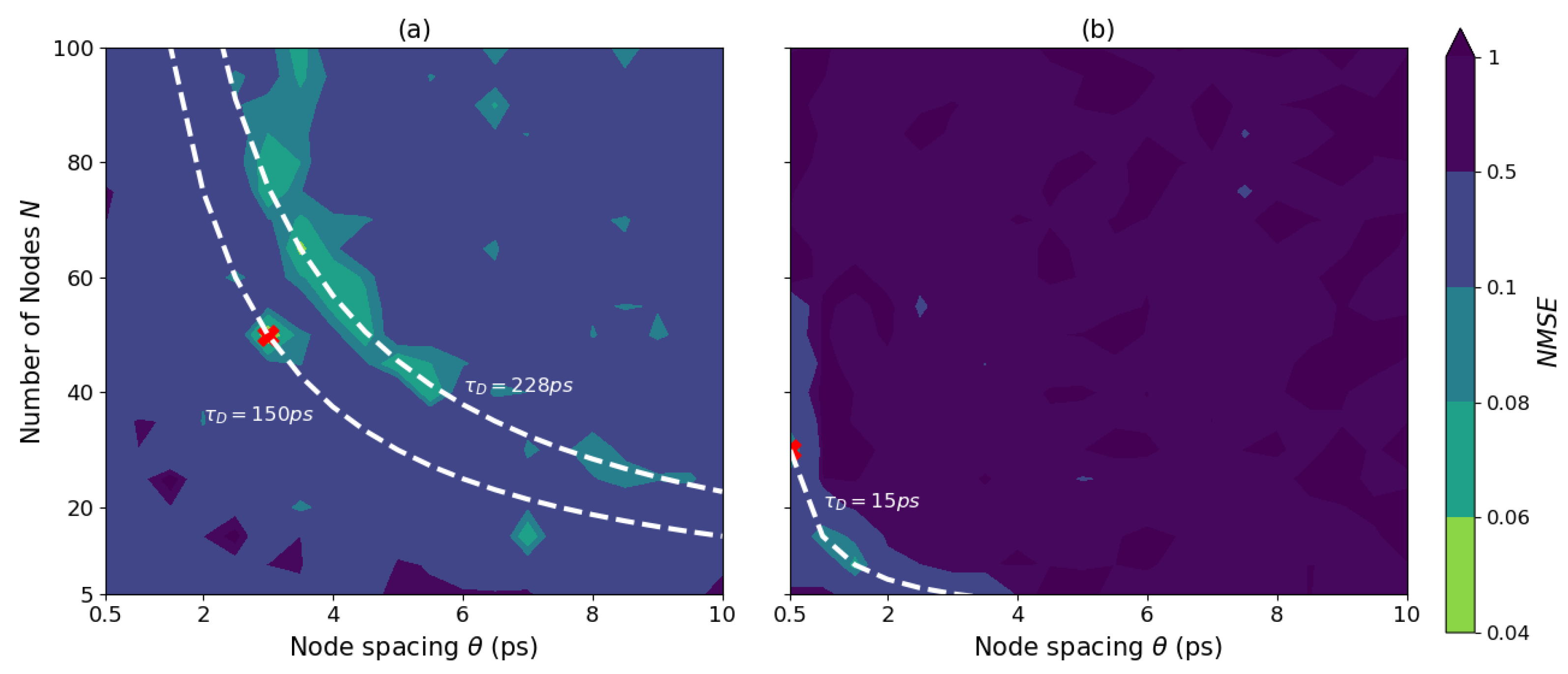
3.1. The Role of Delay Time
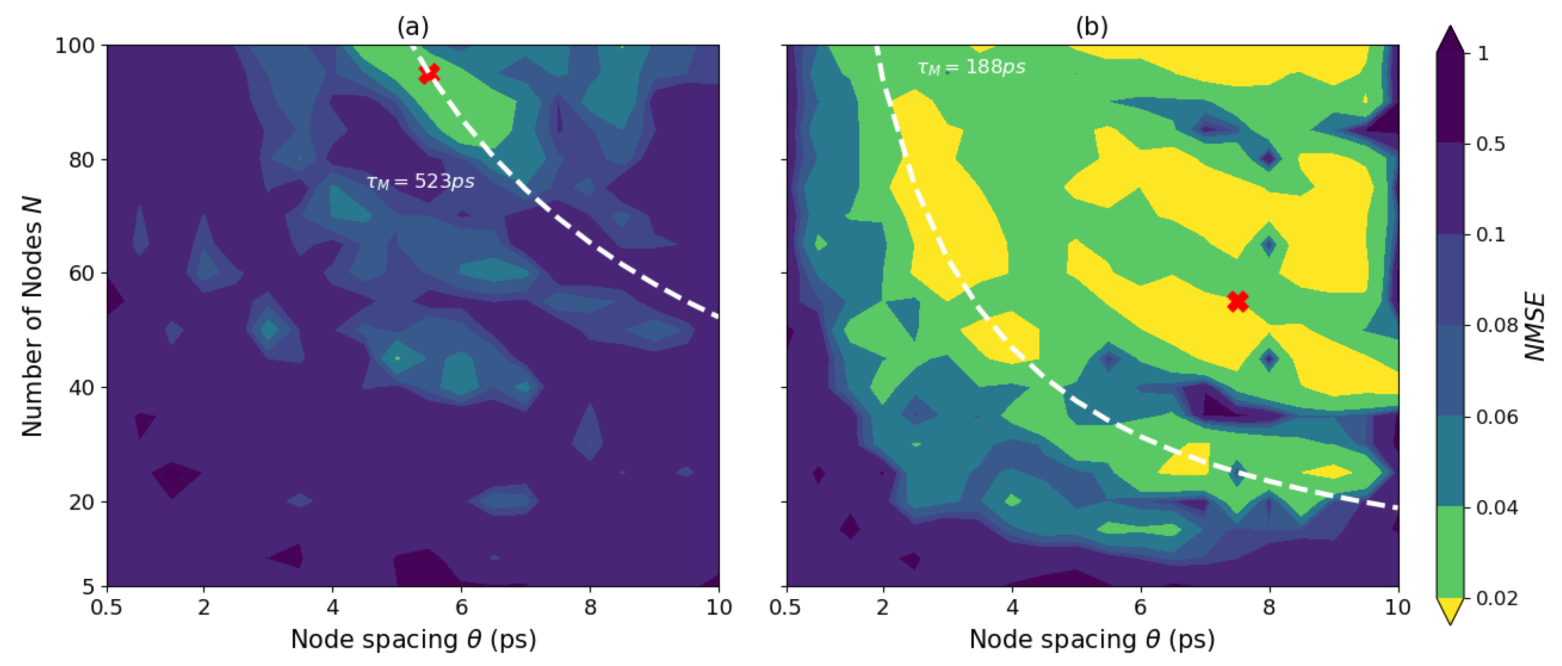
 τ D

In previous studies, the delay time τ D is often matched to the mask length τ M [14,17,18,19]. Initially, we did the same, such that τ D = τ M . This allowed us to observe the effects of feedback-induced dynamics (related to τ D ) on the performance and at the same time we could find a combination of N and θ that might work for our benchmark task ( τ M = N θ ). In Figure 2a,b, we saw the results of these scans for a low feedback rate η = 1 ns 1 and for a high feedback rate η = 100 ns 1 , respectively. For the system with a low feedback rate, we saw a rather large area with good performance (lighter colors) in contrast with the results for the system with a high feedback rate. We would expect the best performing regions to be aggregated at higher values of N and around a particular value of θ , because the node state diversity becomes poor at low N and the node spacing has to be around the period of the polarization oscillations. Here, we see two contrasting plots for the different feedback rates. For η = 1 ns 1 , the absolute best performance was achieved at N = 50 and θ = 3 ps with N M S E = 0.044 . For η = 100 ns 1 , the absolute best performance was achieved at N = 30 and θ = 0.5 ps with N M S E = 0.071 . These best points were shown as red crosses in Figure 2a,b.
On both plots, we see the regions with good performances (lighter colors) that coalesce around hyperbolic curves, corresponding to constant mask length τ M and the delay time τ D , as τ D = τ M . For the low feedback system, we found the best performance at τ D = τ M = 150 ps and a larger region of good performance at τ D = τ M = 228 ps. These are shown as white dashed lines in the left plot. For the strong feedback system, we found the best performance at τ D = τ M = 15 ps, shown as a white dashed line in the right plot. We observe that longer delay lines are required to obtain good performance for a low feedback rate and vice versa. Furthermore, for low feedback rates, the best performances are found near the middle of the hyperbolic line, showing a trade-off between the number of nodes N and the node spacing θ . For high feedback rates, a similar trend is seen, where the performance worsens as the number of nodes N is decreased. This makes sense as the diversity of states of the virtual nodes is reduced if N is too small and hence the nonlinear memory capacity of the system will deteriorate [30].
It seems that the delay time, in combination with the feedback rate, has a very profound effect on the performance of our setup via feedback-induced dynamics. This is in stark contrast with previous delay-based RC setups using edge-emitting semiconductor lasers, where the delay time τ D had no such significant role in the RC performance [20,31].
The results indicate that τ D and η affect the dynamical regime of the VCSEL considerably. This observation was supported by the findings in [32], where the nonlinear dynamics of the spin-VCSEL subjected to feedback was studied. The authors found that VCSELs connected to longer delay lines quickly move towards chaotic regimes with increasing feedback rates, whereas VCSELs connected to shorter delay lines would have various plateaus of steady state behavior, interspersed between chaotic regions, as the feedback rate is increased.
To further investigate the effect of τ D and η on the dynamical regime, we prepared two RC systems with the optimal parameters corresponding to the red crosses in Figure 2a,b. We studied the modal output power as the system was injected with a constant value instead of masked data. The resulting orbit diagrams of the modal output power, as the feedback rate was varied, are shown in Figure 3a,b. In Figure 3a, we see the orbit diagram for a long delay time τ D = 150 ps. The laser has a steady state behavior for the lowest feedback rate, but it quickly moves towards a chaotic regime via a period-doubling route. In contrast, for a shorter delay line τ D = 15 ps (orbit diagram shown in Figure 3b), we see plateaus of steady state behavior, interspersed by periodic regimes, similar to findings in [32].
In Figure 3c,d, we show the Santa Fe timeseries prediction performance as a function of the feedback rate for τ D = 150 ps and τ D = 15 ps, respectively. Furthermore, we show the performance for each possible output layer. From both plots, it is clear that the best performances were achieved when the output layer consists of virtual nodes from both P + and P , whereas training on virtual nodes from a single mode gives the worst outcome. Training on the output polarization P O L o u t = P + P P + + P is not recommended either, since its performance is almost always worse. We see a brief interval for η [ 50 , 80 ] in Figure 3c,d where the output layer formed by the output polarization has a better performance than the rest. However, this performance is nowhere near the minimum N M S E .
From the literature, we know that the best performing reservoirs are typically tuned to be at the edge of a periodic or chaotic dynamical regime before data are injected into the system [3,33,34]. It is at η = 1 ns 1 for τ D = 150 ps and η = 100 ns 1 for τ D = 15 ps, where we see a switch from a steady state to a periodic regime. These are also the feedback rates with which we achieve the best N M S E values. Another local minimum N M S E was found around η = 15.5 ns 1 for τ D = 15 ps in Figure 3d, which corresponds to a switch from a steady state regime to a periodic regime in Figure 3b.
The findings from Figure 3 confirm our assumption that the delay time τ D and feedback rate were intrinsically linked to the RC performance as opposed to previous RC setups, where the delay time is several orders of magnitude larger, and where the delay can be kept fixed when the feedback rate is changed [14,17,18,27].

3.2. Decoupling τ D and τ M

Now that we established that the delay time τ D is intrinsically linked to the RC performance, we decouple the mask length τ M from the delay time τ D , such that we can find the optimal number of nodes N and optimal node spacing θ . There have already been studies where the delay time was longer than the mask length ( τ D > τ M ), with state-of-the-art performances [16,20,31]. This mismatch between mask length and delay time is favorable for RC performances, because the interconnection between nodes over multiple round trips becomes more complex. In our case, however, the delay time τ D is already fixed at rather low values. For the reservoir with weak feedback, the delay time is fixed at τ D = 150 ps and for the reservoir with strong feedback at τ D = 15 ps. Here, we expect that the case where τ D < τ M will be favored, since τ M = N θ and we need a sufficient number of nodes N to be able to perform the tasks.
We did the same parameter scan as in Figure 2, but this time with constant delay times ( τ D = 150 ps for η = 1 ns 1 and τ D = 15 ps for η = 100 ns 1 , corresponding to the white lines in Figure 1) and the results are shown in Figure 4. We again see the best performing regions coalesce along hyperbolic curves only corresponding to a constant mask length τ M this time. For the reservoir with low feedback, we find the best performance N M S E = 0.025 at θ = 5.5 ps and N = 95 , corresponding to τ M = 522.5 ps. This point was depicted with a red cross in Figure 4. The mask length at this point corresponds to a processing speed of approximately 2 GSa/s.
For the reservoir with strong feedback, shown in Figure 4b, we have a considerably larger part of parameter space which gives excellent performance. The best performance for this reservoir is N M S E = 0.012 , found at θ = 7.5 ps and N = 55 , corresponding to τ M = 412.5 ps. This point is depicted with a red cross. However, we observe another region with similar performances ( N M S E around 0.015) around the hyperbolic curve corresponding to τ M = 188 ps (shown as a white dashed line). The points on this white curve have a shorter mask length and hence a higher processing speed as compared to the red cross. The processing speed for the points on this white line is 5.3 GSa/s, almost three times faster than that of the RC with low feedback. Both based on the N M S E as well as the processing speed, we found that our RC has superior qualities when operated with strong feedback rates.
It is worth noting for the discussion later on, that at the best processing speed, a single masked datapoint traverses the delay line τ M τ D = 3.5 times for the low feedback setting and 12.5 times for the high feedback setting.
We also note that the lower left corner of Figure 4 shows high N M S E values, i.e., worse performances, which corresponds to the area where τ D < τ M . In this region, either the number of nodes are not sufficient to deliver the nonlinear memory capacity needed to perform the task or the node spacing becomes too small for the laser to be able to follow the input data. These findings are similar to those in [20]. Similarly, in Figure 4b, we see the lower left corner turn darker, indicating worsening performances. This area is smaller, given that the delay time τ D = 15 ps is smaller than τ D = 150 ps in Figure 4a.

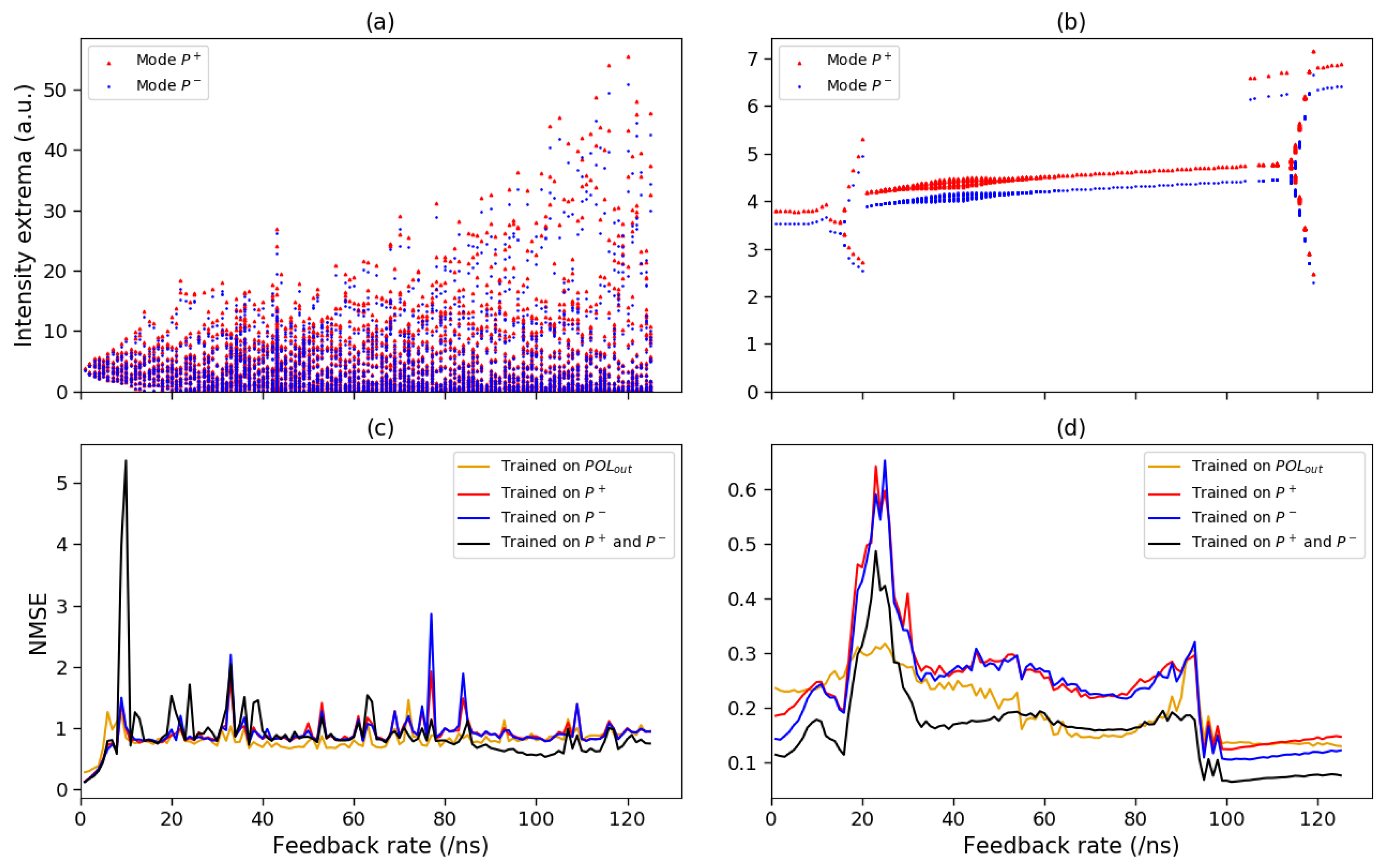
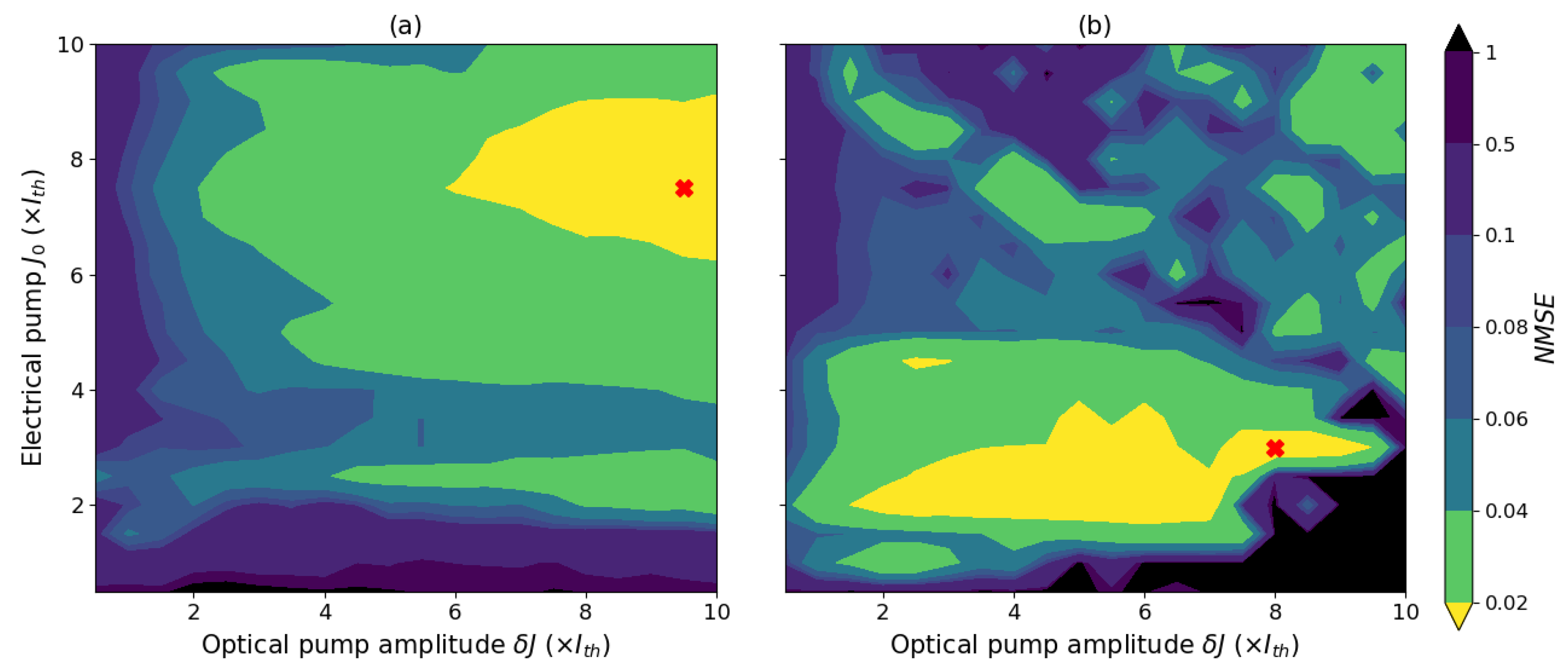
3.3. The Role of Pumping Parameters

Two other important parameters of the RC system are the electrical pump J 0 and the optical pump amplitude δ J . We scanned these two parameters, for a reservoir with weak feedback and a reservoir with strong feedback corresponding to the red crosses in Figure 4a,b. The result of this scan is shown in Figure 5a,b, respectively. We observe that the best performance for the reservoir with weak feedback is found at higher electrical bias as well as higher spin pump amplitude. For the reservoir with strong feedback, the best performances are found at lower electrical biases and a fairly wide interval of optical pump amplitudes (between 2 J t h and 8 J t h ). The points of best performances are indicated by the red crosses. For the low feedback reservoir, this point, corresponding to an N M S E of 0.015 , was found at an electrical pump of 7.5 J t h and an optical pump amplitude of 9.5 J t h . For the high feedback reservoir, the lowest N M S E = 0.013 was found at an electrical pump of 3 J t h and an optical pump amplitude of 8 J t h .
The pump parameters are optimized to rather high values for the reservoir with weak feedback and to low values for the reservoir with strong feedback. We presumed that these optimized parameter sets are such that there is a balance between the linear and nonlinear memory capacity needed for the Santa Fe task. In Ref. [31], in the case of a standard semiconductor laser, Köster et al. showed that the linear memory capacity drastically decreases as the mask becomes longer than the delay time. In our reservoirs, both with weak and strong feedback, the mask is longer than the delay time, namely τ M = 3.5 τ D for weak feedback and τ M = 12.5 τ D for strong feedback. The nonlinear memory capacity in these systems increases, since nodes related to one data sample (i.e., within one mask length) strongly mix with each other due to the mask looping around the delay line multiple times. This increase in nonlinear memory capacity comes at the expense of linear memory capacity, which is typically due to the interaction between nodes of subsequent data samples (i.e., over subsequent mask lengths). However, contrary to the system studied in [31], which have two characteristic timescales (namely the nodal response timescale and the feedback dynamics timescale), our system has three characteristic timescales that can couple nodes with each other. The first of these is the timescale introduced by the polarization dynamics, which governs the nodal response. The second is the timescale introduced by the feedback dynamics, which couples nodes separated by the delay time τ D and lastly, we have the timescale introduced by relaxation oscillations (ROs). The RO frequency and damping are strongly influenced by the pumping parameters.
We prepared two reservoirs to look at the effect of ROs on the interaction between nodes. One reservoir was set up with a weak feedback rate ( η = 1 ns 1 and τ D = 150 ps) and another with a strong feedback rate ( η = 100 ns 1 and τ D = 15 ps). The other parameters of these reservoirs were optimized for best performance in the Santa Fe task. Both systems were injected with a constant stream of zeros until they reached a steady state regime. Then, we applied a perturbation of length θ and observed how this perturbation rippled through the system into the sum of the modal intensities.
The result is shown in Figure 6, where we showed the total output intensity response for the reservoir with weak feedback (in blue) and for the reservoir with strong feedback (in orange). For the sake of the discussion, we plotted the output versus the time in multiples of the mask length ( τ M ), meaning that the blue curve ( τ M = 522.5 ps) is slightly compressed compared to the orange curve ( τ M = 412.5 ps). In addition, we noted that the perturbation has a duration θ , which was different for both optimized systems, namely θ = 5.5 ps for the weak feedback reservoir (blue curve) and θ = 7.5 ps for the strong feedback reservoir (orange curve). The oscillations found in the output of the weak feedback reservoir and strong feedback reservoir had frequencies of around 10 GHz and 5 GHz, respectively. This corresponds to typical RO frequencies found for VCSELs operated at given pump parameters. Furthermore, we see that the RO frequency and the damping increase as the pump parameters are increased.
For the reservoir with weak feedback (blue curve in Figure 6), we see that the response to the perturbation is short-lived. The perturbation introduced at the start of the data sample has an effect over approximately one mask-length. This means that the nodes related to one data sample (i.e., within one mask length) were interacting with each other thanks to the RO, but also nodes between subsequent samples (i.e., over subsequent mask lengths) interact with each other at the edges of the samples. The linear memory capacity that is lost due to the mask looping 3.5 times around the delay line is somewhat reinstated by the interaction between nodes of subsequent samples due to the RO.
For the reservoir with strong feedback (orange curve in Figure 6), we see that the response lingers in the system for at least two subsequent data samples. The mask loops for 12.5 times around the delay time, drastically decreasing the linear memory capacity according to Ref. [31], however, we see that the pumping parameters were optimized such that the RO damping rate was low and hence nodes over multiple samples could still interact with each other, which will counteract the decrease in linear memory capacity.
To conclude this section, we observed that the weak and strong feedback reservoirs could be fine tuned to give better performances, by adjusting the pumping parameters that affect the relaxation oscillations, which on its turn affects how nodes within (and over multiple) mask lengths interact with each other. Further detailed research into the linear and nonlinear memory capacities of the system can be useful to further interpret these results, but such a study is outside the scope of this paper.

4. Conclusions

We numerically investigated a delay-based reservoir computer using a spin-VCSEL, taking advantage of the high modulation speeds achievable with these lasers. We systematically scanned the RC performance as a function of the delay time, the mask length and the pumping parameters. In contrast with known photonic delay-based RC systems, this RC with spin-VCSELs shows a rather strong relation between the delay time and feedback rate on one hand and the RC performance on the other hand. A reservoir with weak feedback has better performances at longer delay times and vice versa for a reservoir with strong feedback. We further observe that the weak (strong) feedback regimes also favor different pumping parameters. We found that the reservoir with strong feedback has superior qualities, both based on the RC performance and the processing speed.
The RC system is benchmarked using the Santa Fe timeseries prediction task and has shown performances comparable to state-of-the-art delay-based RC systems, but at a considerable faster processing speed. The speed reached with this setup is around 5 GSa/s, an improvement by a factor of 10 compared to delay-based RC using single-mode semiconductor lasers [18,20], while maintaining the same error rate. The optimal node spacing is found to be between 5 and 8 ps, which is of the same order of magnitude as the inverse of the used birefringence (5 ps). Since the speed of this system is linked to the birefringence of the lasing cavity, the processing speeds can be increased in the future as the expertise on tuning the birefringence improves.

Author Contributions

Conceptualization, K.H., G.V. and G.V.d.S.; methodology, K.H.; software, K.H.; validation, K.H.; formal analysis, K.H.; investigation, K.H.; resources, K.H.; data curation, K.H.; writing—original draft preparation, K.H.; writing—review and editing, K.H., G.V. and G.V.d.S.; visualization, K.H.; supervision, G.V. and G.V.d.S.; project administration, K.H.; funding acquisition, G.V. and G.V.d.S. All authors have read and agreed to the published version of the manuscript.

Funding

This research was funded by the Research Foundation Flanders (FWO) under the grants G028618N, G029519N and G006020N.

Acknowledgments

We would like to thank Kathy Lüdge and Felix Köster from the Institute of Theoretical Physics of TU Berlin for interesting discussions.

Conflicts of Interest

The authors declare no conflict of interest.

References

  1. Manyika, J.; Chui, M.; Brown, B.; Bughin, J.; Dobbs, R.; Roxburgh, C.; Hung Byers, A. Big Data: The Next Frontier for Innovation, Competition, and Productivity; McKinsey Global Institute: Washington, DC, USA, 2011. [Google Scholar]
  2. Araujo, F.A.; Riou, M.; Torrejon, J.; Tsunegi, S.; Querlioz, D.; Yakushiji, K.; Fukushima, A.; Kubota, H.; Yuasa, S.; Stiles, M.D.; et al. Role of non-linear data processing on speech recognition task in the framework of reservoir computing. Sci. Rep. 2020, 10, 1–11. [Google Scholar]
  3. Van der Sande, G.; Brunner, D.; Soriano, M.C. Advances in photonic reservoir computing. Nanophotonics 2017, 6, 561–576. [Google Scholar] [CrossRef]
  4. Tanaka, G.; Yamane, T.; Héroux, J.B.; Nakane, R.; Kanazawa, N.; Takeda, S.; Numata, H.; Nakano, D.; Hirose, A. Recent advances in physical reservoir computing: A review. Neural Netw. 2019, 115, 100–123. [Google Scholar] [CrossRef] [PubMed]
  5. Lugnan, A.; Katumba, A.; Laporte, F.; Freiberger, M.; Sackesyn, S.; Ma, C.; Gooskens, E.; Dambre, J.; Bienstman, P. Photonic neuromorphic information processing and reservoir computing. APL Photonics 2020, 5, 020901. [Google Scholar] [CrossRef]
  6. Jaeger, H. Short Term Memory in Echo State Networks; GMD-Forschungszentrum Informationstechnik: Bremen, Germany, 2001; Volume 5. [Google Scholar]
  7. Grigoryeva, L.; Ortega, J.P. Echo state networks are universal. Neural Netw. 2018, 108, 495–508. [Google Scholar] [CrossRef] [Green Version]
  8. Maass, W.; Natschläger, T.; Markram, H. Real-time computing without stable states: A new framework for neural computation based on perturbations. Neural Comput. 2002, 14, 2531–2560. [Google Scholar] [CrossRef] [PubMed]
  9. Maass, W. Liquid state machines: Motivation, theory, and applications. In Computability in Context: Computation and Logic in the Real World; World Scientific: Singapore, 2011; pp. 275–296. [Google Scholar]
  10. Kulkarni, M.S.; Teuscher, C. Memristor-based reservoir computing. In Proceedings of the 2012 IEEE/ACM International Symposium on Nanoscale Architectures (NANOARCH), Amsterdam, The Netherlands, 4–6 July 2012; pp. 226–232. [Google Scholar]
  11. Vandoorne, K.; Mechet, P.; Van Vaerenbergh, T.; Fiers, M.; Morthier, G.; Verstraeten, D.; Schrauwen, B.; Dambre, J.; Bienstman, P. Experimental demonstration of reservoir computing on a silicon photonics chip. Nat. Commun. 2014, 5, 1–6. [Google Scholar] [CrossRef] [Green Version]
  12. Denis-Le Coarer, F.; Sciamanna, M.; Katumba, A.; Freiberger, M.; Dambre, J.; Bienstman, P.; Rontani, D. All-optical reservoir computing on a photonic chip using silicon-based ring resonators. IEEE J. Sel. Top. Quantum Electron. 2018, 24, 1–8. [Google Scholar] [CrossRef] [Green Version]
  13. Brunner, D.; Fischer, I. Reconfigurable semiconductor laser networks based on diffractive coupling. Opt. Lett. 2015, 40, 3854–3857. [Google Scholar] [CrossRef] [Green Version]
  14. Appeltant, L.; Soriano, M.C.; Van der Sande, G.; Danckaert, J.; Massar, S.; Dambre, J.; Schrauwen, B.; Mirasso, C.R.; Fischer, I. Information processing using a single dynamical node as complex system. Nat. Commun. 2011, 2, 1–6. [Google Scholar] [CrossRef] [PubMed] [Green Version]
  15. Paquot, Y.; Duport, F.; Smerieri, A.; Dambre, J.; Schrauwen, B.; Haelterman, M.; Massar, S. Optoelectronic reservoir computing. Sci. Rep. 2012, 2, 1–6. [Google Scholar] [CrossRef]
  16. Larger, L.; Baylón-Fuentes, A.; Martinenghi, R.; Udaltsov, V.S.; Chembo, Y.K.; Jacquot, M. High-speed photonic reservoir computing using a time-delay-based architecture: Million words per second classification. Phys. Rev. X 2017, 7, 011015. [Google Scholar] [CrossRef]
  17. Brunner, D.; Soriano, M.C.; Mirasso, C.R.; Fischer, I. Parallel photonic information processing at gigabyte per second data rates using transient states. Nat. Commun. 2013, 4, 1–7. [Google Scholar] [CrossRef] [PubMed] [Green Version]
  18. Nguimdo, R.M.; Verschaffelt, G.; Danckaert, J.; Van der Sande, G. Fast photonic information processing using semiconductor lasers with delayed optical feedback: Role of phase dynamics. Opt. Express 2014, 22, 8672–8686. [Google Scholar] [CrossRef] [PubMed]
  19. Harkhoe, K.; Van der Sande, G. Delay-based reservoir computing using multimode semiconductor lasers: Exploiting the rich carrier dynamics. IEEE J. Sel. Top. Quantum Electron. 2019, 25, 1–9. [Google Scholar] [CrossRef]
  20. Harkhoe, K.; Van der Sande, G. Task-independent computational abilities of semiconductor lasers with delayed optical feedback for reservoir computing. Photonics 2019, 6, 124. [Google Scholar] [CrossRef] [Green Version]
  21. Takano, K.; Sugano, C.; Inubushi, M.; Yoshimura, K.; Sunada, S.; Kanno, K.; Uchida, A. Compact reservoir computing with a photonic integrated circuit. Opt. Express 2018, 26, 29424–29439. [Google Scholar] [CrossRef]
  22. Harkhoe, K.; Verschaffelt, G.; Katumba, A.; Bienstman, P.; Van der Sande, G. Demonstrating delay-based reservoir computing using a compact photonic integrated chip. Opt. Express 2020, 28, 3086–3096. [Google Scholar] [CrossRef]
  23. San Miguel, M.; Feng, Q.; Moloney, J.V. Light-polarization dynamics in surface-emitting semiconductor lasers. Phys. Rev. A 1995, 52, 1728. [Google Scholar] [CrossRef]
  24. Martin-Regalado, J.; Prati, F.; San Miguel, M.; Abraham, N. Polarization properties of vertical-cavity surface-emitting lasers. IEEE J. Quantum Electron. 1997, 33, 765–783. [Google Scholar] [CrossRef] [Green Version]
  25. Gahl, A.; Balle, S.; Miguel, M.S. Polarization dynamics of optically pumped VCSELs. IEEE J. Quantum Electron. 1999, 35, 342–351. [Google Scholar] [CrossRef]
  26. Lindemann, M.; Xu, G.; Pusch, T.; Michalzik, R.; Hofmann, M.R.; Žutić, I.; Gerhardt, N.C. Ultrafast spin-lasers. Nature 2019, 568, 212–215. [Google Scholar] [CrossRef]
  27. Vatin, J.; Rontani, D.; Sciamanna, M. Experimental reservoir computing using VCSEL polarization dynamics. Opt. Express 2019, 27, 18579–18584. [Google Scholar] [CrossRef]
  28. Guo, X.X.; Xiang, S.Y.; Zhang, Y.H.; Lin, L.; Wen, A.J.; Hao, Y. Polarization multiplexing reservoir computing based on a VCSEL with polarized optical feedback. IEEE J. Sel. Top. Quantum Electron. 2019, 26, 1–9. [Google Scholar] [CrossRef]
  29. Weigend, A.S.; Gershenfeld, N.A. Results of the time series prediction competition at the Santa Fe Institute. In Proceedings of the IEEE International Conference on Neural Networks, San Francisco, CA, USA, 28 March–1 April 1993; pp. 1786–1793. [Google Scholar]
  30. Dambre, J.; Verstraeten, D.; Schrauwen, B.; Massar, S. Information processing capacity of dynamical systems. Sci. Rep. 2012, 2, 1–7. [Google Scholar] [CrossRef] [PubMed]
  31. Köster, F.; Ehlert, D.; Lüdge, K. Limitations of the Recall Capabilities in Delay-Based Reservoir Computing Systems. Cogn. Comput. 2020, 1–8. [Google Scholar] [CrossRef]
  32. Song, T.; Xie, Y.; Ye, Y.; Liu, B.; Chai, J.; Jiang, X.; Zheng, Y. Numerical Analysis of Nonlinear Dynamics Based on Spin-VCSELs with Optical Feedback. Photonics 2021, 8, 10. [Google Scholar] [CrossRef]
  33. Boedecker, J.; Obst, O.; Lizier, J.T.; Mayer, N.M.; Asada, M. Information processing in echo state networks at the edge of chaos. Theory Biosci. 2012, 131, 205–213. [Google Scholar] [CrossRef] [PubMed]
  34. Chrol-Cannon, J.; Jin, Y. On the correlation between reservoir metrics and performance for time series classification under the influence of synaptic plasticity. PLoS ONE 2014, 9, e101792. [Google Scholar] [CrossRef] [Green Version]
Figure 1. (left) Schematic overview of our setup, consisting of a spin-VCSEL connected to a feedback line with delay τ D . The spin-up and spin-down populations are pumped separately by J + and J , respectively. (right) A simplified plot showing the input data I ( t ) in blue, the masked input data A ( t ) in red and the timescales of τ M and θ .
Applsci 11 04232 g001
Figure 2. Santa Fe timeseries prediction performance, indicated by the N M S E , color-coded unto the parameter space spanned by N and θ for (a) η = 1 ns 1 and (b) η = 100 ns 1 . The delay time was fixed to match the mask length, τ D = τ M . The red crosses denote the minimum N M S E achieved over the scanned space and the white dashed lines are a guide to the eye, denoting a constant delay time τ D and hence constant mask length τ M .
Applsci 11 04232 g002
Figure 3. Orbit diagram of the modal output power as the feedback rate η is varied for (a) τ D = 150 ps and (b) τ D = 15 ps. The N M S E for the Santa Fe timeseries prediction task as the feedback is varied for (c) τ D = 150 ps and (d) τ D = 15 ps.
Applsci 11 04232 g003
Figure 4. Santa Fe timeseries prediction performance, indicated by the N M S E , color-coded unto the parameter space spanned by N and θ for (a) τ D = 150 ps and η = 1 ns 1 , and (b) τ D = 15 ps and η = 100 ns 1 . The red crosses denote the minimum N M S E achieved over the scanned space and the white dashed lines are a guide to the eye, denoting a constant mask length τ M τ D .
Applsci 11 04232 g004
Figure 5. Santa Fe timeseries prediction performance, indicated by the N M S E , color-coded unto the parameter space spanned by the electrical pump J 0 and the optical pump amplitude δ J for (a) η = 1 ns 1 , τ D = 150 ps, N = 95 and θ = 5.5 ps and (b) η = 100 ns 1 , τ D = 15 ps, N = 55 and θ = 7.5 ps. The red crosses denote the minimum N M S E achieved over the scanned space.
Applsci 11 04232 g005
Figure 6. A reservoir with weak and another one with a strong feedback rate are prepared with a constant injection of zeros. A perturbation is introduced in the first node of the second datapoint and we observe how this perturbation ripples through the sum of the modal intensities. Parameters for the reservoir with weak feedback: η = 1 ns 1 , τ D = 150 ps, N = 95 , θ = 5.5 ps, J 0 = 7.5 J t h and δ J = 9.5 J t h and for the reservoir with strong feedback: η = 100 ns 1 , τ D = 15 ps, N = 55 , θ = 7.5 ps, J 0 = 3 J t h and δ J = 8 J t h .
Applsci 11 04232 g006
Table 1. List of paramaters, designation and values used in the simulations for delay-based RC using the SFM.
ParameterSymbolValue
Linewidth enhancement factor α 5
Carrier decay rate γ 1 ns 1
Photon lifetime τ p 1.54 ps
Spin decay rate γ s 450 ns 1
Linear dichroism γ a −1.16 ns 1
Linear birefringence γ p 200 π GHz
Amplitude saturation factor ϵ a 1.6
Phase saturation factor ϵ p 3.2
Electrical pump J 0 2 J t h , unless mentioned otherwise.
Optical pump amplitude δ J 6 J t h , unless mentioned otherwise.
Constant feedback phase Ω 0
Mask length τ M τ M = N θ
Delay time τ D scanned from 2.5 ps to 1 ns
Feedback rate η scanned from 1 to 100 ns 1
Number of nodesNscanned from 5 to 100
Node spacing θ scanned from 0.5 to 10 ps
Publisher’s Note: MDPI stays neutral with regard to jurisdictional claims in published maps and institutional affiliations.

