Simplified Numerical Analysis of Soil–Structure Systems Subjected to Monotonically Increasing Lateral Load

Abstract

Numerical modelling of the soil in seismic design of structures is always a daunting task. The goal of this article is to develop a simplistic numerical modelling technique for shallow founded buildings on compliant soils. An existing large-scale experimental research (TRISEE) was used for calibration. The physical model comprised of a rigid square foundation placed on a sand bed connected to a rigid column and was subjected to a dynamic sine loading. The results from the TRISEE experiment are well known and commonly used by researchers in this field, yet none of the numerical studies were conducted considering the loose sand case. Nonlinear link elements and linear springs were used for representing the soil. It was determined that the soil behavior is highly influenced by the stiffness, selected hysteresis model, and the p-y curve. Considering the software limitations, numerical models represent the experimental behavior in a good manner. Based on the results obtained from the experiment, a case study on a steel frame building with SSI effects included was conducted. Considering the results from this research, the authors recommend implementation of SSI effects into the building’s design phase since they exhibit unfavorable impacts on the seismic behavior and can lead to underdesigned structural elements. However, it has to be emphasized that certain limitations exist due to simplified modelling approaches that were used for this research.

1. Introduction

Experimental research usually presents a valuable insight into the effects of soil–structure interaction (SSI), yet due to high costs it is not always conducted. Some valuable SSI experimental results and sand modelling techniques on including SSI effects in soil–structure systems are available in literature [1,2,3]. These types of experiments can be conducted statically or dynamically and in large or small scale, but considering the significant costs of this type of experiments, small scale experiments are more common. Most of the small-scale experiments are conducted in geotechnical centrifuges [3,4,5,6,7,8,9,10] which result in severe use of interpretation scaling factors of the experimental results. Large scale experiments, on the other hand, are commonly conducted using shaking tables [1,3] or as static or cyclic experiments [2,11,12]. For any SSI experiment, large-scale experiments are encouraged [13,14] since they describe the behavior of structures more accurately than their small-scale counterparts. Furthermore, the research on buildings with shallow foundations founded on compliant soils is of great importance since a large number of buildings are built in this manner [15,16].

One of the available large-scale SSI experiments on compliant soils is TRISEE [12,17,18,19]. Set of large-size experiments was designed to investigate the nonlinear interaction between buildings with shallow foundations and compliant soils during cyclic loading. More information regarding this experiment can be found in the following chapters.

What is more, performance based seismic design requires complex numerical modelling to reflect the realistic behavior of a building. To achieve this notion, not only structural systems but also foundation soil should be modelled appropriately. It is well known that buildings founded on rock behave differently than buildings on soft soils during seismic events [20,21,22,23]. It is not uncommon in nowadays design practice to model buildings fixed at the base, which is certainly not true for buildings founded on soft soils. During a seismic event, buildings founded on compliant soils can incline, rock, or slide, which in most cases results in seismic energy dissipation that can be interpreted as a mechanism for building protection [24,25,26]. Therefore, in some cases, the soft soil layer can function as a seismic isolator under the building, although one must be careful when determining beneficial or detrimental soil effects on the building [26]. To conduct research in the field of soil–structure interaction, both the structural and geotechnical design aspects have to be studied and appropriate simplifications for the structure and soil have to be used.

Since many buildings are designed without considering SSI, the purpose of this study is to more closely examine how SSI affects the seismic response of a building and how to include it in the non-linear static methods of analysis (like for example the pushover analysis), which are widely used by practicing engineers due to the relatively high degree of accuracy and low computational cost [27,28,29,30]. It should be noted that soil–structure interaction effects in pushover analysis have already been studied by other researchers to some extent [30,31,32,33,34,35]. The research comprised in this article present simplified approaches for the modelling of the soil–structure systems tested on large-scale experiments. The proposed modelling approach is further applied to two two-dimensional frames under nonlinear static analysis. The results obtained on soil–structure systems are compared to results on the structure itself which give valuable conclusions regarding the effect of the soil on the frame using simplified modelling methods.

2. Large Scale Experiment

The research of non-linear soil–structure interaction under simulated seismic loading was conducted within the TRISEE research project. The project was carried out in the late 1990s and it comprised of several different large-scale experiments. The structure model included of a rigid steel column and a slab representing typical shallow footing. The column was used to introduce simulated seismic loading into the model. Through the column, horizontal force and overturning moment simulating the inertial loads were transmitted to foundations. The research programme included experiments conducted on dense and on loose sand with the relative density D_r of 85% and 45%, respectively. Ticino sand is a uniform coarse-to-medium silica sand with D₅₀ = 0.55 mm, coefficient of uniformity, C_u = 1.6, specific gravity, G_s = 2.684, e_min = 0.579, e_max = 0.931 and constant volume frictional angle, ${\phi }_{cv}=35°$, Poisson’s ratio equal to ν = 0.30. The calculation of dynamic soil properties incorporated sand shear wave velocity taken from [12], $v_s=220 \raisebox{1ex}{$\mathrm{m}$}\!\left/ \!\raisebox{-1ex}{$\mathrm{s}$}\right.$ for dense sand, and $v_s=185 \raisebox{1ex}{$\mathrm{m}$}\!\left/ \!\raisebox{-1ex}{$\mathrm{s}$}\right.$ for the loose sand case. Square footing of 1.00 × 1.00 m in plane, 0.20 m in thickness was embedded to the depth of 1.00 m so that the overburden pressure was simulated. The column of the model was modelled as 0.12 × 0.12 m in cross section and 1.00 m in height. The model was made of steel with elasticity modulus equal to E = 210,000 $\raisebox{1ex}{$\mathrm{N}$}\!\left/ \!\raisebox{-1ex}{${\mathrm{mm}}^2$}\right.$. 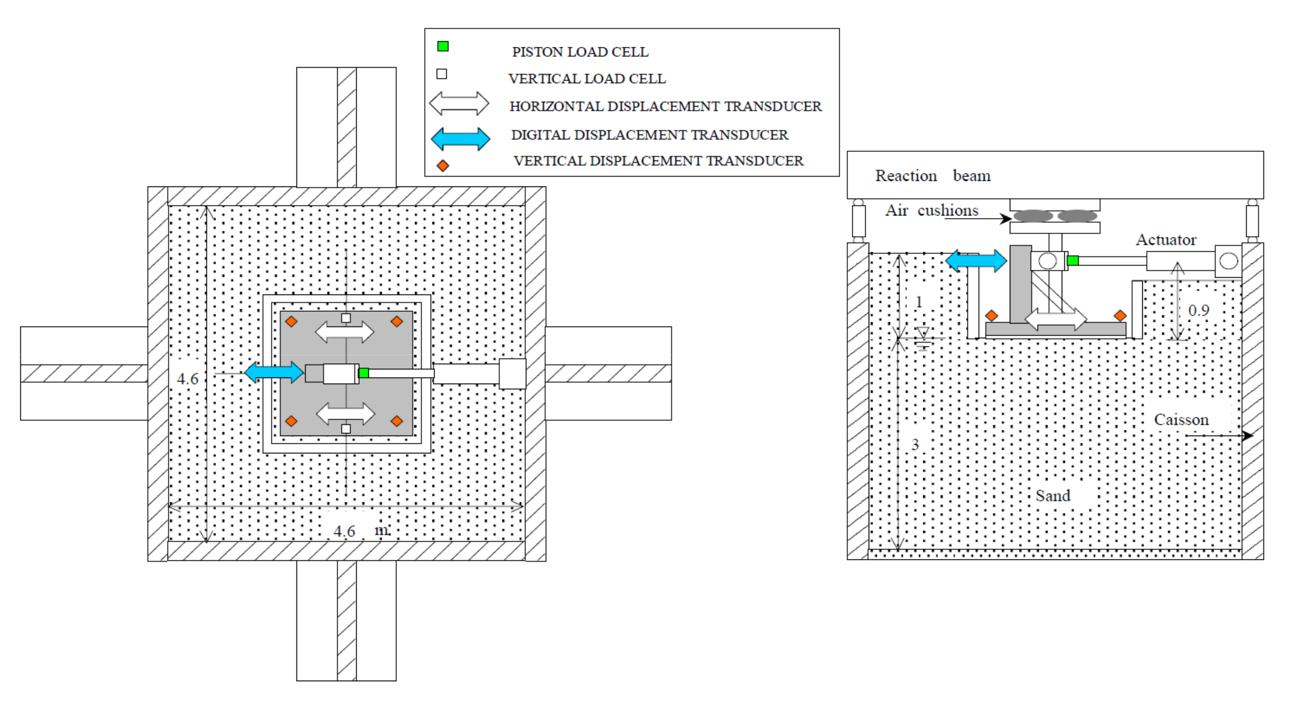A large sand box, measuring 4.60 × 4.60 m in plan and 4.00 m in height (Figure 1) was constructed. Saturated Ticino sand was used to simulate the soil.

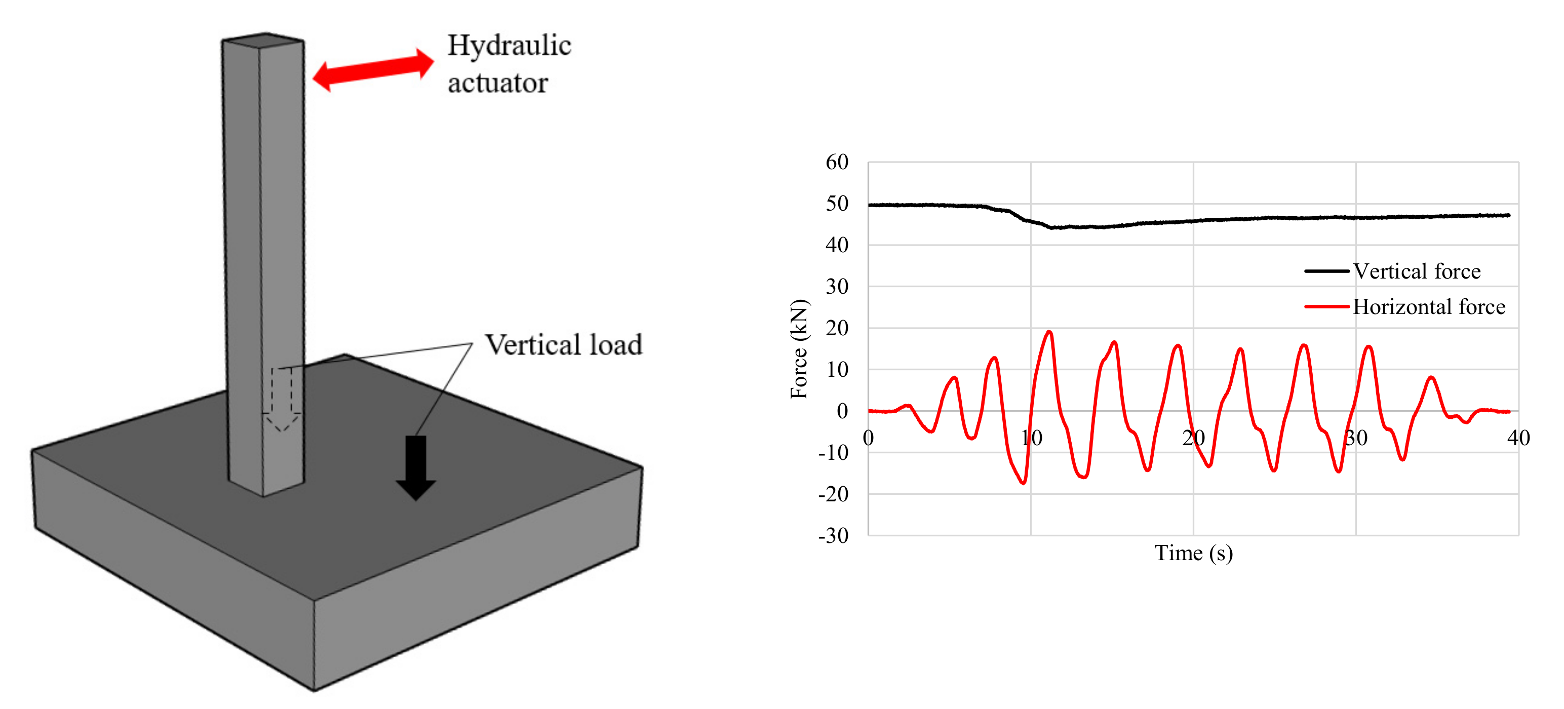
The model founded on loosely built-in sand was loaded with 100 kN of vertical load, while the model founded on dense sand was loaded with a vertical force equal to 300 kN. In both cases, the vertical load applied was considerably lower than the soil load bearing capacity. The vertical load was introduced to the model using air cushions and a reaction beam while the horizontal cyclic load was applied at the top of the column using a hydraulic actuator. The vertical load was firstly applied to the model as it represents the weight of the superstructure. After the full vertical load was applied, cyclic load was introduced to the model as presented Figure 2. The cyclic load was applied to the model in three series, starting with small amplitude force-controlled cycles in Phase I, followed by application of earthquake-like time history loading in Phase II and finished with sinusoidal displacement cycles of increasing amplitude.

The experimental model was examined by two groups of instruments. The first group of instruments embedded into the sand was used for the assessment of the initial soil conditions. Following sensors were placed in the soil: 9 small geophones which were used to measure saturation of the soil, 6 thermal and 6 electrical probes for the local check. The soil was tested by three cone penetration tests (CPT) performed by a standard cone with 35.7 mm in diameter. Moreover, body-wave velocities were measured during the different phases of sample preparation. A second group of instruments was used for observation of the foundation. Applied forces, horizontal and vertical displacements of the foundation, total and effective soil pressures underneath the foundation were monitored. The following sensors were installed: 11 load cells for horizontal and vertical stresses in the soil, 2 mini-piezometers for measuring the water pressure, 5 pressure cells underneath the foundation, 4 vertical displacement transducers at the corners of the foundation to measure settlements and rotations, 2 horizontal transducers in the foundation, a digital transducer to measure the horizontal displacement of the actuator, 2 load cells for the vertical force and 1 load cell (in the piston) for the horizontal force.

For this research the authors used the Phase II record and the setup comprising the structure founded on the loose sand.

3. Numerical Modelling of the SSI System

In the scope of the research at hand, the model tested within the TRISEE project was modelled using the finite element analysis software SAP2000 v21.0.2 [36]. The physical model of the structure was modelled in 3D using shell finite elements representing the foundation slab and frame elements representing the column. The loading curve recorded during the experiment was applied at the top of the column as a horizontal cyclic loading.

Multilinear plastic links were used to simulate the soil compliance in the vertical direction. The foundation model was supported by 25 identical link elements. Vertical stiffness of the soil was calculated according to Gazetas [37] and Mylonakis et al. [38] which are presented in Equations (1)–(3). According to this proposal, the axial stiffness of the spring is a function of the soil’s shear modulus (G), Poisson ratio (ν), and geometry of the foundation strip (L,B) where L is half of the foundation strip length and B is half of the foundation strip width.

$$k_x=k_y-\frac{0.2\cdot G\cdot L}{0.75-\nu }\cdot \left(1-\frac{B}{L}\right)$$

(1)

$$k_y=\frac{2\cdot G\cdot L}{2-\nu }\cdot \left[2+2.5\cdot {\left(\frac{B}{L}\right)}^{0.85}\right]$$

(2)

$$k_z=\frac{2\cdot G\cdot L}{1-\nu }\cdot \left[0.73+1.54\cdot {\left(\frac{B}{L}\right)}^{0.75}\right]$$

(3)

Multilinear links require information regarding the force–deformation backbone curve as well as the hysteresis type for the soil. The backbone curve was determined according to Rees and Van Impe [39] briefly presented in Figure 3 and Equations (4)–(7). A step-by-step detailed procedure for the backbone curve calculation in sand can be found in [40]. The damping ratio of the soil could have been included into the numerical model within the vertical link elements, but it was neglected, since it did not have a significant impact on results, such as settlement or tilting of the foundation. In the particular case, the inclusion of damping did not to have a significant impact on overall results for the soil–structure system since it was loaded with relatively slow cycles of loading.

$$p_{ult}=\overline{A_s}·p_s$$

(4)

$$p_m=\overline{B_s}·p_s$$

(5)

$$p=k_{py}·z·y_k$$

(6)

$$p_{st}=\gamma ·z·\left[\frac{k_0·z tan\phi sin\beta }{\tan \left(\beta -\phi \right)·cos\alpha }+\frac{tan\beta }{\tan \left(\beta -\phi \right)}·\left(b+z·tan\beta ·tan\alpha \right)+k_0·z·tan\beta ·\left(tan\phi ·sin\beta -tan\alpha \right)-k_{\alpha }·b\right]$$

(7)

To simulate the hysteretic behavior of the soil-foundation system the Takeda model [41] was chosen from the available hysteretic models in the software. This model was primarily developed for the purpose of modelling the response analysis of reinforced concrete structures, yet due to similarities in the shape of the curve to the response of the sand, it can be also used for soil modelling. In recent years it has been successfully implemented to model the nonlinear response of soils [42]. The compression part of the hysteresis loop is modelled by force–deformation (p-y) curve (Figure 3.) while the tension part is neglected. It is important to stress out that use of simplified modelling approaches leads to certain limitations, therefore, initial imperfections of the soil–structure system are not included in the numerical model as well as saturation of the foundation soil.

Gap elements and horizontal linear springs are assigned along the edges of the model. As the foundation model is symmetrical, both, the stiffness in x and y direction have the same properties (Figure 4).

The model was loaded with three different time-dependent functions. Two functions simulated gravitational loading in the vertical direction and one function simulated seismic loading in the horizontal direction. The vertical load was applied directly on the foundation slab, while the horizontal load was applied at the top of the column. The recorded loading curve taken from the TRISEE experiment was imported to the numerical model as a Time history load.

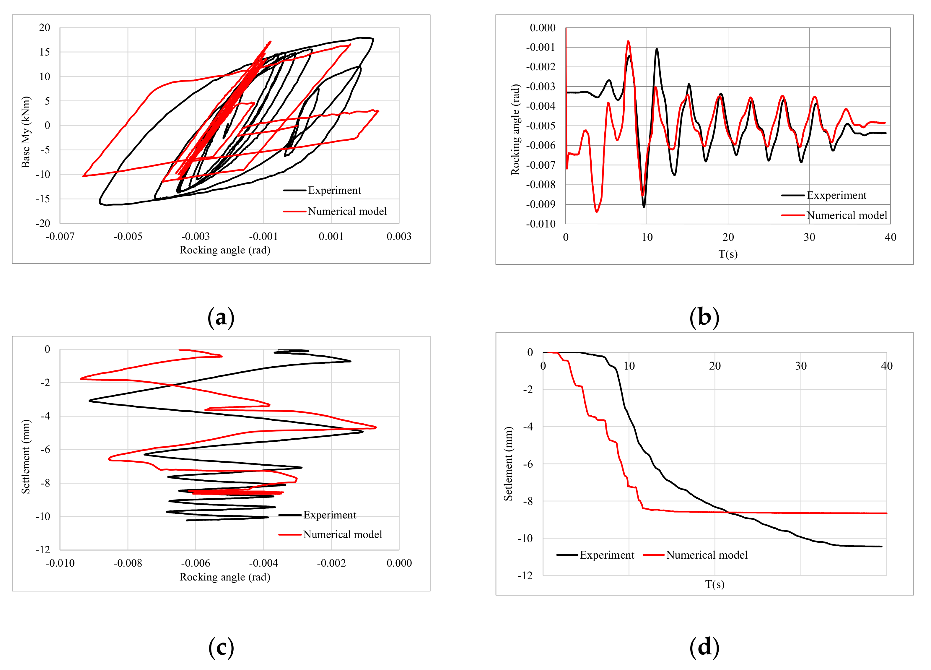
The comparison of experimental and numerical results (Figure 5) is presented through: (a) rocking angle–overturning moment curve; (b) time–rocking angle curve; (c) rocking angle–settlement curve; and (d) time–settlement curve. Observing Figure 5, it can be concluded that rocking of the foundation in the numerical model matches well with the experimental results, although the settlement of the foundation shows a difference in the numerical model (8.50 mm) and experiment (10.00 mm). Moreover, rocking of the foundation shows significant difference at the beginning until the plasticity of foundation soil is reached when the amplitude of rocking is matched well with the experiment.

A preliminary parametric study showed that the numerical results are highly sensitive to both the shape of the force–displacement backbone curve and the hysteretic model selected to simulate the soil behavior. It is important to emphasize that the structural model of the experimental setup was not fully horizontally leveled when placed on the sand bed. It was assumed that tilting of the model resulted with plasticity of the sand on one end of the foundation. The model was tilted by around 2° in the loading direction which resulted in a horizontal shift of the top of the column by 3.33 mm. The implementation of an initial tilting in the numerical model would consider the adoption of additional assumptions, therefore tilting was not implemented into the numerical model. Furthermore, limitations of this numerical model have to be stressed out. The numerical model, specifically the model of the soil represent dry sand conditions in contrary to the experiment with saturated soil under the foundation. The saturation of the sand could be included into Equations (1)–(3) only by varying the Poisson’s ratio which was determined not to have a large impact on the numerical results. Moreover, as it was mentioned earlier, imperfections of the model placement on the foundation soil were not included in the numerical model. With all this considered, more efficient numerical models might capture experimental results even more accurately.

Figure 6 shows the comparison between the numerical and experimental horizontal displacement of the top of the column in the direction of the applied horizontal load. To exclude the tilting of the physical model, numerical results were shifted by 3.33 mm in the direction of the horizontal load.

After the occurrence of pronounced plasticity under the action of the maximum horizontal force the numerical model describes the behavior of the experimentally tested model with a large degree of accuracy. In spite of all of the above, the hysteretic cycles in the moment-rocking angle, as well as rocking time-history and vertical settlement time history describe the behavior of the experimentally tested model with satisfactory accuracy, as shown in Figure 5.

4. Numerical Case Study—Assessment of SSI Effects on a Steel Building

The conclusions acquired within numerical and experimental research presented in earlier chapters were further assessed on a building designed according to Eurocode regulations under a nonlinear static analysis. Nonlinear static analysis was chosen because of its low computational costs and significant numerical accuracy. The building was designed without the consideration of SSI effects by Castro and Elghazouli [43]. The steel frame building comprised of five stories with composite steel–concrete slabs. Seismic capacity of the building has already been extensively analyzed in the two doctoral theses [43,44], and is used herein for calibration of the structural numerical model shown in Figure 8. The columns are regularly spaced with 9.0 m of spacing in both directions and are oriented to form a moment resisting frame in X-direction and a braced frame in Y-direction as shown in Figure 7. The columns and beams are made of HEB and IPE steel cross-sections (mild structural steel S275) to suit the provisions of Eurocodes 3, 4, and 8 (Figure 7). Structural slabs are assigned with 2.0 kN/m² of additional dead load and 3.0 kN/m² of live load. The building was designed by considering foundations on rock (Ground Type A) with a design peak ground acceleration (PGA) of 0.30 g.

In order to study the SSI effects on frames, a moment resisting frame and a braced frame were studied as separate two-dimensional (2D) frames. The moment resisting frames are flexible and exhibit a frame behavior while the braced frames acquire higher stiffness potentially representing the behavior of shear walls. Since the observed building is regular in plane and in elevation, designed not to suffer the high impact of three-dimensional (3D) effects, it is possible to research such building frames in 2D as it was already done in the literature [45,46,47]. The frames are firstly observed as fixed at the base and later with foundations and the links representing the compliance of the soil. Numerical models were made in the SAP2000 v21.0.2 software [36].

4.1. Moment Resisting Frame

4.1.1. Fixed-Base Moment Resisting Frame

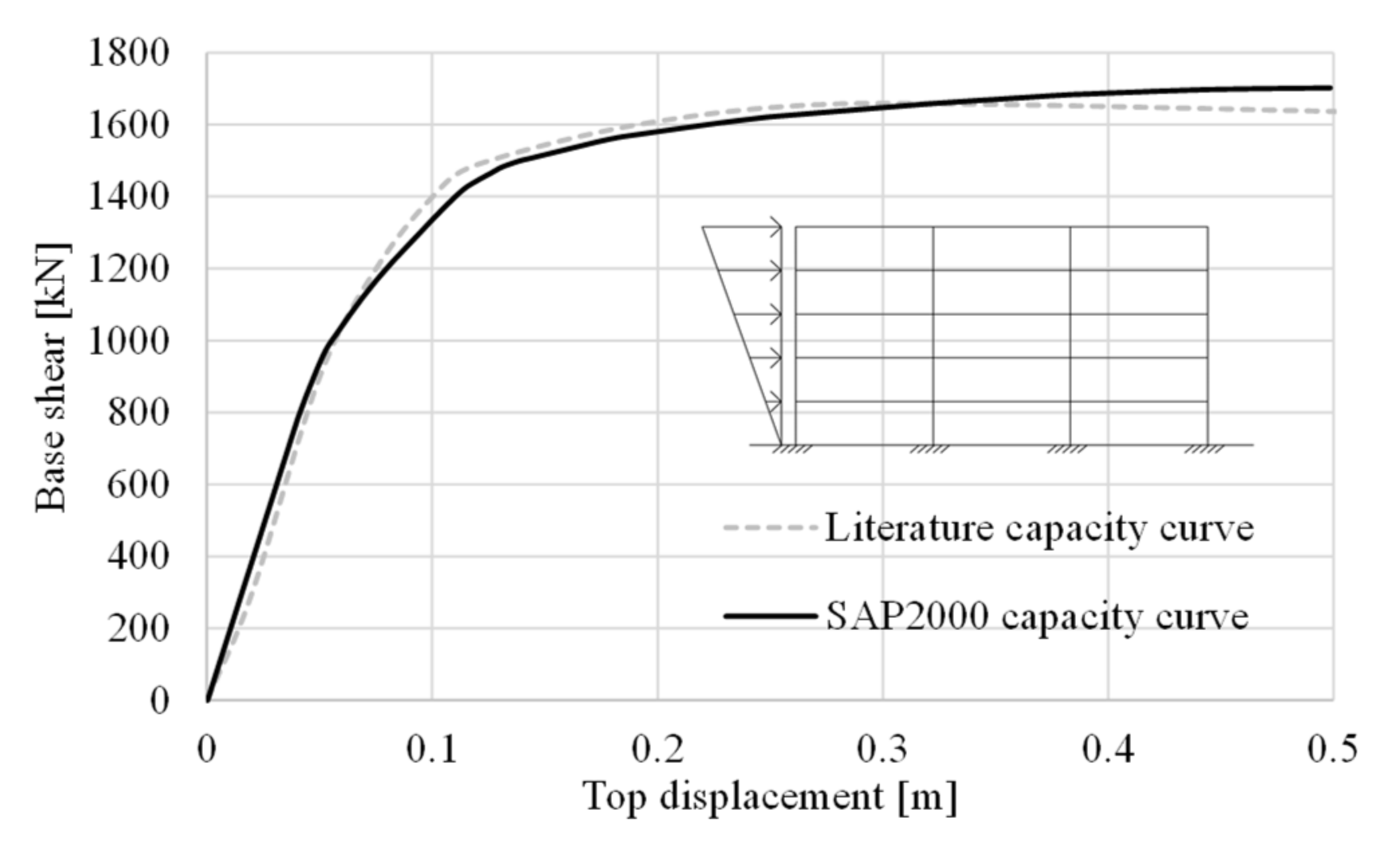
The numerical model of the moment resisting frame (MRF) is modelled in accordance with the data given in [43,44]. A simple frame model without composite connections and slabs was made using frame elements. The first period of vibration (T₁) for this model equals to 1.0 s [43]. Since literature [43,44] provides detailed information about the geometry, material model, mass distribution, and lateral force distribution, it was therefore possible to calibrate the numerical model to match the capacity curve to the one presented in [44], as showed in Figure 8.

Material non-linearity was considered in the form of lumped plasticity, consisting of plastic hinges in columns and beams, modelled in accordance with Eurocode 8—Part 3. Plastic hinges were modelled with a trilinear moment–rotation relationship, while the yielding (M_y) and plastic moment (M_p) were determined for each cross section and floor separately and assigned manually as presented in

Table 1. Calculated plastic hinge properties.

Cross-Section	Story	My (kNm)/Mp (kNm)	θy/θp
HEB 340	1, 2, 3, 4, and 5	593/662	0.004/0.026
HEB 450	1, 2, 3, 4, and 5	976/1095	0.003/0.019
IPE 500	1, 2, 3, 4, and 5	530/603	0.009/0.05

. The building loads were assigned to the frame model as uniform loads. The loads were composed of the self-weight, considered by the software, and linear vertical loads on the frames due to actions on the slabs, additional 45.0 kN/m of dead load and 27.0 kN/m of live load. In order to match the capacity curve presented in [43] an identical triangular lateral load distribution to Castro and Elghazouli [43] was used. The effective seismic mass of the building was composed of 100% dead load and 30% of live load.

In Table 1 the M_y and M_p are given, along with the corresponding yielding rotation (θ_y) and plastic rotation (θ_p). Since the building was designed following the capacity design principle, the inelastic deformations first occur in the beams (strong columns–weak beams principle).

4.1.2. Moment Frame with SSI Effects

To incorporate SSI effects, shallow single foundations were designed by following the provisions of Eurocode 7 (EC7) [48] and the Croatian national annex [49]. According to the national annex for EC7 in Croatia, design approach number three should be used for the design.

The soil properties were taken from the local river sand. Sand was determined to be uniform when it was tested in geotechnical laboratory, detailed results can be found in [50]. The properties that are used for this research are for the compacted sand case: density 1550 kg/m ³, shear wave velocity 135 m/s, and Poisson ratio 0.3.

Under each column, single foundations with layout dimensions 3.60 × 3.60 m and a depth of 1.0 m were considered. Foundations are numerically modelled as reinforced concrete shell elements under each column connected with a foundation frame beam 0.80 m wide, 0.50 m high, and 5.40 m long.

Horizontal stiffness of the soil around the foundation were represented by linear horizontal springs determined according to Gazetas [37] and Mylonakis et al. [38]. Every single foundation was modeled with two horizontal springs for each direction (

Table 2. Total spring stiffnesses.

Spring Stiffness Direction	Stiffness (N/m2)
x, y	4.57 × 108
z	3.55 × 108

). Vertical soil stiffness was represented by nonlinear link elements which were assigned soil properties determined for local river sand following the steps described in Section 3. There were nine vertical links total under every single foundation.

Furthermore, two different lateral load distributions were used for the numerical models founded on the soil. Firstly, a lateral load distribution in the analysis corresponding to the first mode of oscillation and second, uniform lateral load distribution. Modal lateral load distribution is encouraged to be used for SSI systems as shown in [51]. In

Table 3. Lateral load distributions for the moment resisting frame.

Story	Modal Distribution (N)		Uniform Distribution (N)
	Fixed Base	Model on the Soil	Fixed Base	Model on the Soil
Foundation	-	0.5	-	50
1st story	10.4	11.3	50	50
2nd story	24.3	24.7	50	50
3rd story	36.5	36.6	50	50
4th story	45.5	45.3	50	50
5th story	50.5	50.2	50	50

one can find information regarding the forces applied on the model. The comparison of the capacity curves for each case will benefit explaining the effects of the lateral load distributions on the results.

Figure 9 presents capacity curves obtained within the numerical calculations for the moment resisting frame system on the soil. Differences in the capacity and stiffness are noticeable but further conclusions will be made when the effects of the load distribution will be studied on the structure elements separately.

4.2. Braced Frame

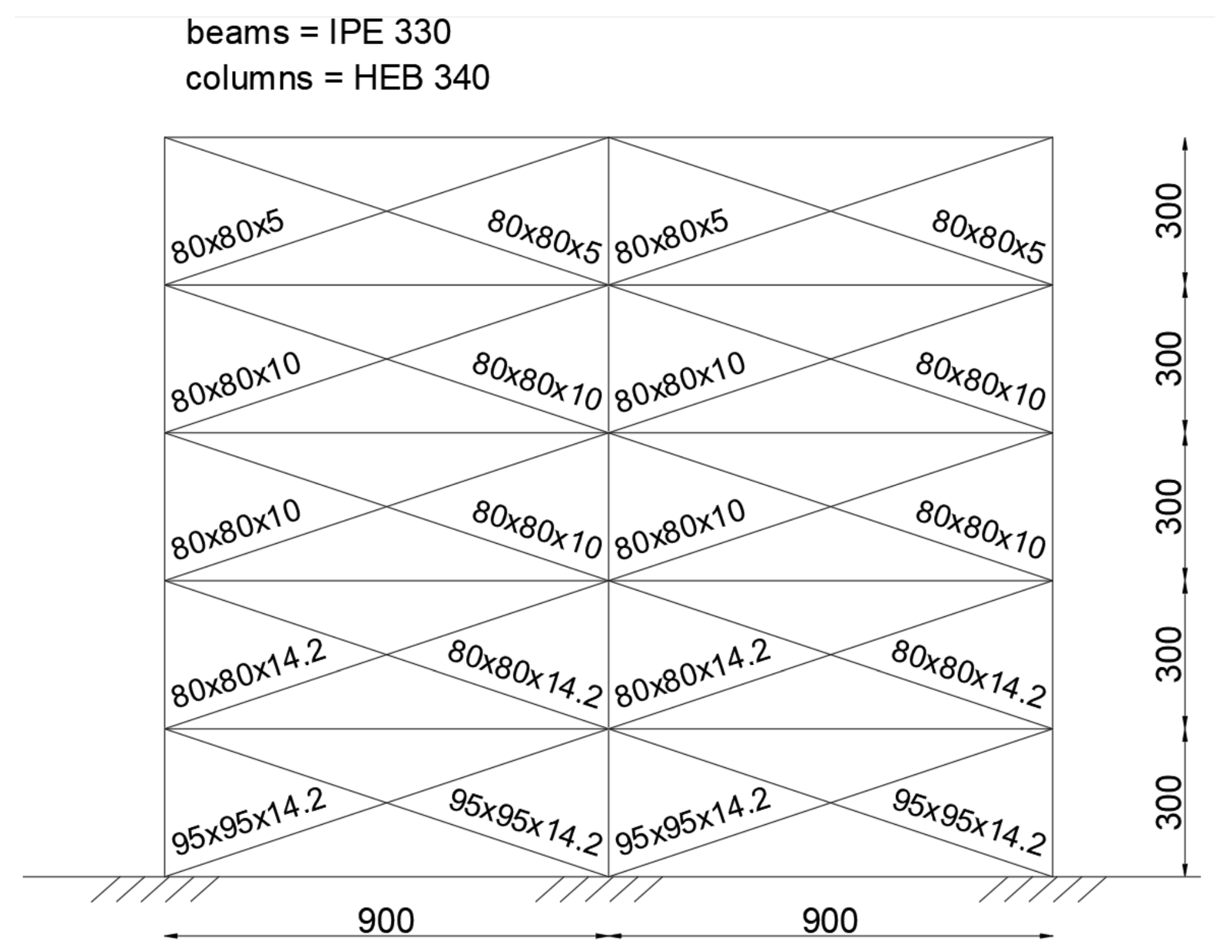
In the final step of the numerical study, the braced frame (BF) from the Y-direction of the building was also studied to assess the SSI effects on this structural typology. When braced frames are subjected to horizontal actions, their displacements, interstory drifts and internal force distributions resemble the behavior of shear walls rather than the moment resisting frame.

4.2.1. Fixed-Base Braced Frame

Since in the observed literature [43,44] only the moment resisting frame was analyzed, the information regarding the placement and geometry of the bracing system was not given. Therefore, the equivalent seismic force approach was used for the design of the braces. The selected braces are shown in Figure 10. It was decided to use hollow steel tubes with a square cross-section that were designed according to Eurocode 8 by fulfilling the code-based bracing criteria [45,52]. Bracing was placed only on the external frames while the inner frames were left without bracing. This research deals with examination of one external frame. It is important to emphasize that most of the dead and live loads in the building are carried by the moment resisting frames. Braced frames are loaded with self-weight and also with nodal forces coming from seismic load combination from the slabs at the nodes connecting columns and beams. Nodal forces are calculated to be 235 kN for the middle nodes and 117 kN for external nodes for seismic combination of the forces. Plastic hinges, described in

Table 4. Braced frame plastic hinge properties.

Cross-Section	Story	My (kNm)/Mp (kNm)	θy/θp	χ
HEB 340	1, 2, 3, 4 and 5	178/271	0.007/0.039	1
IPE 330	1, 2, 3, 4 and 5	196/221	0.013/0.08	1
Cross-section	Story	+N(kN)/−N(kN)	Δt(mm)/Δc(mm)
80 × 80 × 5	5	412.5/113.58	6.21/1.71
80 × 80 × 10	3 and 4	770/189.74	6.21/1.53
80 × 80 × 14.2	2	1027.68/231.38	6.21/1.39
95 × 95 × 14.2	1	1262.1/406.12	6.21/1.99

, were calculated for all cross-sections and assigned to the model. The bracing is designed only to withstand axial loads. Pushover analysis was performed for two different types of lateral load distributions as it was done in previous chapters for the moment resisting frame.

If the bracing cross sections are observed, the hinges are compound of compressive and tensile axial limits parallel with deformations of tensile force Δt and compressive force Δc.

4.2.2. Braced Frame with SSI

The braced frame with added foundation, vertical nonlinear links, and horizontal linear springs was studied. Single foundations under each column connected with foundation beams were added as it is presented in Section 4.2 and recommended according to EC7. Since the soil properties and geometry of the foundation did not change, the spring and link properties are the same as presented in Section 4.1.2.

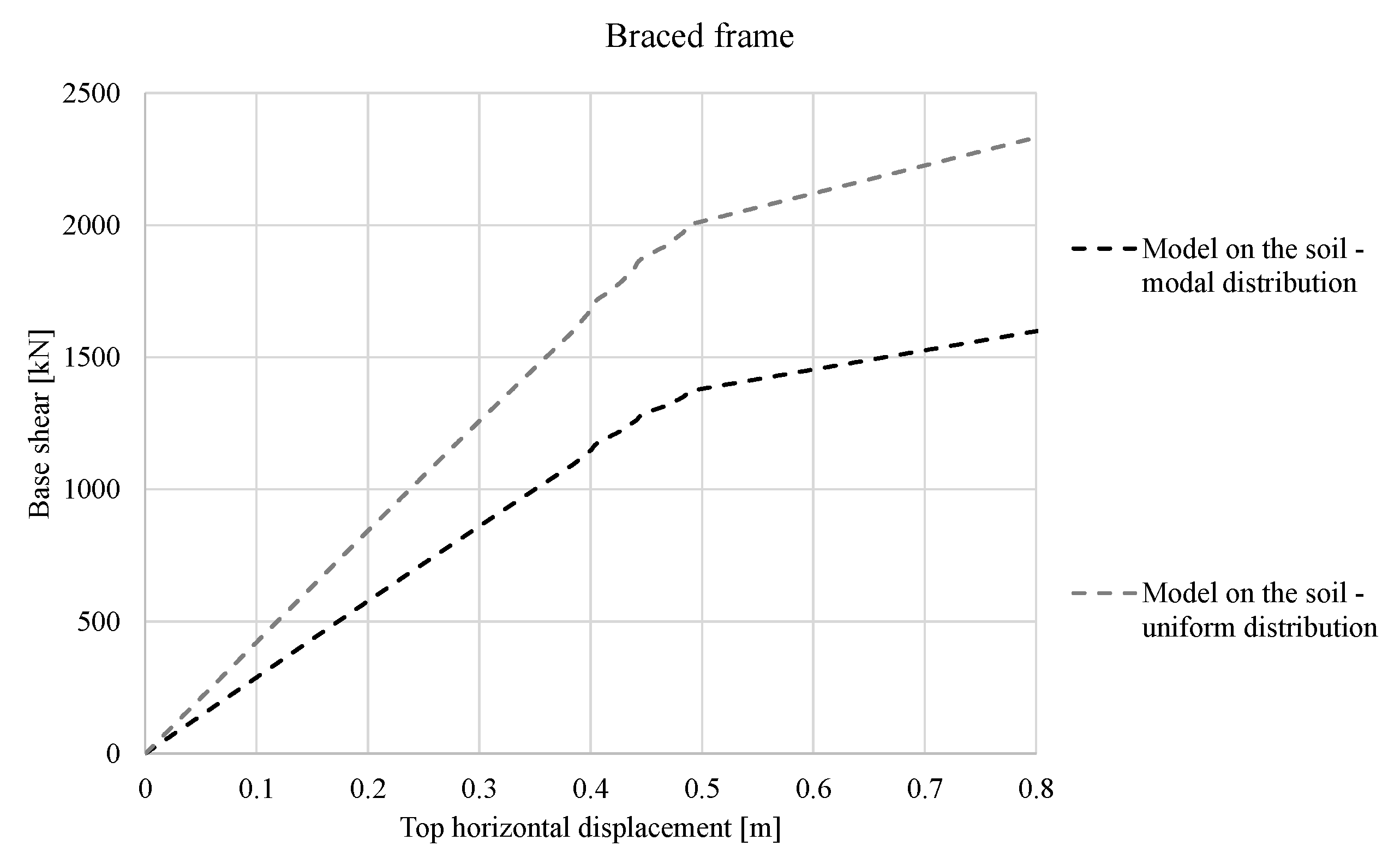
The braced frame was loaded with two different lateral load distributions as shown in

Table 5. Lateral load distributions for braced frame.

Story	Modal Distribution (N)		Uniform Distribution (N)
	Fixed Base	Model on the Soil	Fixed Base	Model on the Soil
Foundation	-	1.6	-	50
1st story	16.3	18.2	50	50
2nd story	36.1	36.7	50	50
3rd story	58.8	57.1	50	50
4th story	76.7	74.4	50	50
5th story	94.3	91.5	50	50

. The results obtained within the numerical analyses are compared in Figure 11.

The comparison of the capacity curves is presented in Figure 11 and it is possible to conclude the same tendencies as for the moment resisting frames are repeated. The coupled system with soil that is loaded with an uniform lateral load distribution is showing higher capacity and stiffness which is a result of the additional force at the foundation level that is significantly larger when compared to the foundation force for the modal lateral load case.

5. Comparison and Discussion

The main objective of the comparative case study was to assess the extent of SSI effects on two different steel typologies (MRF and BF) in order to learn how different structural systems and lateral load distributions are affecting the overall seismic response of the analyzed topologies.

Changes in the story drift for different levels of peak ground acceleration (PGA) were observed. The target displacements for each seismic acceleration were determined based on the N2 method [53]. Limit values of the story drifts for the two analyzed typologies are given in terms of limit states by Eurocode 8—Part 3 [54] or FEMA as follows: (i) Damage limitation (DL or IO), (ii) Significant damage (SD or LS), and (iii) Near collapse (NC or CP). According to Croatian annex, two limit states should be observed, which means that a return period of 475 years should be checked for the SD limit state and a return period of 95 years for the DL limit state.

The analyzed moment resisting frame was designed without consideration of SSI effects. The building is located on a moderately active seismic area with a peak ground acceleration (PGA) equal to 0.22 g and a soft soil site that corresponds to sub-soil of class D in accordance with Eurocode 8—Part 1 [52].

A comparison between the pushover curves of the SSI system (coupled systems) is already presented in Section 4. The capacity curves for both lateral load distributions are plotted in Figure 9 and Figure 11.

Changes of the capacity for the moment resisting frame (MRF) coupled systems present an increase of the capacity up to 25% when uniform load distribution is compared to the modal lateral load distribution. Uniform and modal lateral load distributions for the braced frame (BF) on the soil resulted with differences in the capacity up to 35%.

Furthermore, Figure 12 presents the story drift for a seismic event with a 475-year return period. When the MRF is observed, increase in the story drifts for the systems on the soil are highlighted. Substantial differences are found in higher stories, while the lower stories present a smaller increase for the soil systems. It is important to emphasize that fixed-base model loaded with uniform load showed larger drifts than allowed within the Eurocode regulations. When the soil is included, the damage limit is not reached. In other hand, there are no safety reserves when the soil is taken into consideration.

It is noticed that a large increase of the story drifts is found for the BF of the soil compared to fixed-base BF, especially for the modal lateral load distribution which exceeds the significant damage (SD) state according to Eurocode. This implies that BF is underdesigned if the soil part of the system is considered. Damage within the building floors is kept similar for each lateral load distribution case when the frame is modelled as fixed at the base and founded on compliant soil. Overall, comparing the two lateral load distributions for MFR and BF, larger story drifts are distinguished for the modal lateral load distribution than the uniform load distribution no matter the foundation case.

Results for the incremental N2 method are presented in Figure 13. The PGA was increased incrementally from zero to 0.50 g, with a step size of 0.05 g. Fixed-base models and models on the soil with varying lateral load distribution were considered. It can be seen from Figure 13, the target displacement for both frames is increased as the PGA increases.

Generally, fixed models have lower target displacement demands compared to coupled systems on the soil. Again, the model with the uniform lateral load distribution is showing lower demand for the same required acceleration for models with modal distribution. Generally, the uniform load distribution is less accurate than the modal distribution since it does not consider the relationships between the modal displacements of each story. Interestingly, larger increase of the demanded target displacement for models on the soil is found for BF compared to MRF. This could potentially lead to the conclusion that frames with higher stiffness are more sensitive to SSI effects.

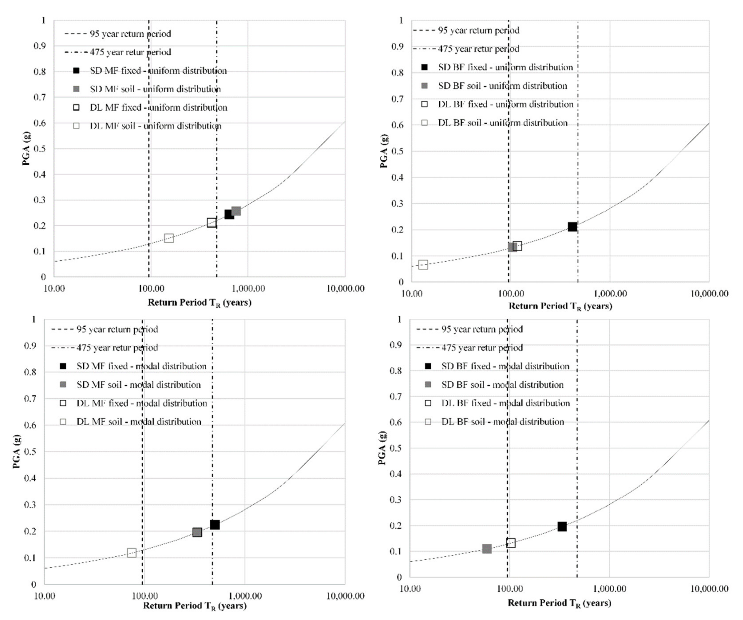
In Figure 14 the results plotted on the site hazard curve expressed as the return period (T_R) vs. the PGA are presented. The points on the curve indicate the PGA value and the corresponding seismic return period when a specific structural model reaches the SD and DL limit state. SSI models resulted in lower peak acceleration and shorter return period which leads to conclusion that fixed-base models are underdesigned.

When modal lateral load distribution for MRF is observed, the numerical models for SD limit state show a decreased peak acceleration of 12% and a return period of 33% compared to the uniform load distribution for MRF where peak acceleration increased 5% and return period 17% for the models on the soil compared to fixed-base cases. If the DL limit state is considered, the peak acceleration is decreased 39% and the return period 78% for the modal distribution, while the uniform distribution shows 29% lower peak acceleration and 64% return period. This goes in hand with the higher story drifts for the modal distribution presented before.

Site hazard was further calculated for each BF model. For the SD limit state, BF on the soil show a decreased peak acceleration of 37% and return period of 75% for uniform distribution compared to fixed-base models while in the case of the modal load distribution the peak acceleration decreased 44% and return period 83%. DL limit state shows a decrease in peak acceleration of 51% and a return period of 89% for uniform load distribution. Modal distribution for BF DL limit state resulted with a decrease of peak acceleration 58% and a return period of 193%.

Overall results show that most of the SD model cases on the soil did not exceed the return period of 475 years, which leads to the concerned conclusion of underdesigned frames. Similar conclusion can be derived for the soil DL cases which drawback the return period of 95 years obligated by Croatian annex.

6. Conclusions

Soil structure interaction (SSI) presents an important aspect in the complex numerical modelling of buildings under seismic actions. Buildings founded on compliant soils can incline rock or slide which result in seismic energy dissipation, while on other hand the increase of the period of oscillation could potentially lead to higher seismic forces. Therefore, one must be careful when determining beneficial or detrimental soil effects on the building.

The goal of this article was to investigate more closely the simplistic SSI modelling parameters and approaches for buildings founded on soft soils represented by sand. Therefore, an existing experimental campaign was studied to learn more about SSI effects and numerical soil modelling. A well-documented experimentally tested model was used to validate the numerical model. The physical model was experimentally tested within the TRISEE project. The physical model comprised of a relatively simple superstructure and a foundation plate. It was founded on a loose Ticino sand embedded in a large rigid tank and subjected to horizontal cyclic loading. Loose sand case of this experiment was not studied or numerically modelled in detail by other authors up to this day.

The soil–structure system was modelled adopting simplified approaches. Simplified numerical models are less time consuming and easily adopted by engineering practice. The soil was modelled using vertical multilinear link elements and the Takeda hysteretic model, while the structure and foundation were modelled using elastic frame and shell elements, respectively. This research shows that for the case of SSI simple numerical models can describe the overall behavior of experimentally obtained data with a satisfactory level of accuracy in the light of rocking of the foundation and energy dissipation in the soil. In contrary, settlement of the foundation soil and behavior of the model in early stages—before plasticity of the soil is achieved—contains larger discrepancies due to imperfections of the experimental setup that were not considered in the numerical model. After the occurrence of pronounced plasticity, under the action of the maximum horizontal force, the numerical model well describes the behavior of the experimentally tested model. In spite of all above, the hysteretic cycles in the moment-rocking angle, as well as rocking time history and the vertical settlement describe the behavior of the experimentally tested model to satisfactory accuracy.

Based on the results from the experimental campaign, a case study on a steel building with SSI effects was conducted. A realistic regular five-story steel building designed according to Eurocode regulations found in literature was used. The building was designed as fixed at the base and within this research a single foundation under every column was added. A local river sand from the Drava river was taken as the foundation soil. The building comprised of regularly spaced columns in both directions oriented to form a moment resisting frame in one direction and a braced frame in perpendicular direction. Frames from both directions separately, were studied within this research. Modal and uniform lateral load distributions were used for both of the numerical models in the fixed-base setup and on the soil. Changes in the story drift and target displacement were observed for different levels of peak ground acceleration. Pushover curves were compared for each load case and the corresponding return periods for the models were calculated. It was concluded that the lateral force distribution is important in terms of SSI effects. Models on the soil showed unfavorable mechanisms. However, an increase of the capacity is noticeable for particular lateral load systems.

Furthermore, the incremental N2 method showed higher target displacements for the coupled systems as in the fixed-base systems. Results indicated on the hazard curve showed that the coupled models result in a lower peak acceleration and shorter return periods, which leads to the conclusion that fixed-base models are underdesigned.

For the observed cases the research has shown an unfavorable effect due to the soil. To get a general conclusion, extended research should be conducted for many different structural typologies and soils. Considering the results from this research the authors recommend the implementation of SSI effects into the design of the buildings.

Nevertheless, it should also be emphasized that due to simplification purposes some assumptions have been made in the conducted research, i.e., the selected hysteresis model and the neglection of damping. Therefore, the presented results should be interpreted in the scope of these assumptions. Furthermore, the research could be further extended by observing the building in 3D under several real seismic events in addition to detailed parametric analyses.