Sizing and Sitting of DERs in Active Distribution Networks Incorporating Load Prevailing Uncertainties Using Probabilistic Approaches

Abstract

In this study, a microgrid scheme encompassing photovoltaic panels, an energy storage system, and a diesel generator as a backup supply source is designed, and the optimal placement for installation is suggested. The main purpose of this microgrid is to meet the intrinsic demand without being supplied by the upstream network. Thus, the main objective in the design of the microgrid is to minimize the operational cost of microgrid’s sources subject to satisfy the loads by these sources. Therefore, the considered problem in this study is to determine the optimal size and placement for generation sources simultaneously for a microgrid with the objectives of minimization of cost of generation resources along with mitigation of power losses. In order to deal with uncertainties of PV generation and load forecasting, the lognormal distribution model and Gaussian process quantile regression (GPQR) approaches are employed. In order to solve the optimization problem, the lightning attachment procedure optimization (LAPO) and artificial bee colony (ABC) methods are employed, and the results are compared. The results imply the more effectiveness and priority of the LAPO approach in comparison with ABC in convergence speed and the accuracy of solution-finding.

1. Introduction

In recent years, the increase in electrical demand, the rise of crude oil and natural gas prices, restructuring and the growth of privatization, and the advent of modern technologies have been led to revolutionary changes in the electricity industry and the assumption of specific attention to distributed generation (DG) technologies [1,2,3]. DG sources or small-scale electricity sources can generate power in the range of 1 kW to 10 MW in the location of the load or in the vicinity of consumption centers. DG technologies bring tangible benefits such as peak clipping (peak shaving), improvement of reliability indices, reduction in power losses due to being close to consumption places, alleviation of voltage drops and improvement of voltage profile, etc., for distribution networks. In addition, the integration of renewable clean energy sources, such as solar, wind, and fuel cell sources, has promoted the power system planners and experts to use these DG units as much as possible [4,5]. The increase in the pervasiveness of DGs and the combined use of various types of DG sources has resulted in the emergence of the microgrid concept. The microgrids are generally defined as small-scale power systems in distribution voltage level encompassing some DGs and some electrical and thermal loads usually accompanied by energy storage systems (ESS) [6,7].

In traditional power systems, the power generation was used to be centralized, and the power flow was always unidirectional from generation and transmission systems toward distribution systems and loads. However, in the recent decade, the structure of power systems has evolved so that modern power systems are experiencing more interest in the use of DG systems at the distribution level [8]. According to the rules and regulations in different countries, various definitions are given based on the place of DG installation, the purpose of use of DG, and their scale of generation (DG sizing). However, a common definition that overlaps all those definitions can be expressed as a small-scale generating unit with limited scalability, which is intended to be used in a distribution network or demand-side [9,10,11,12,13,14,15,16].

Determination of the optimal size of DG units and the optimal place for installation of them is distribution network subject to satisfy all constraints of the grid and minimize the incurred cost to the grid’s operation have assumed particular attention since the last decade. In this regard, a wide diversity of studies is conducted on this subject, and various methods are proposed in order to solve and assess this problem. In [17], a microgrid scheme including a photovoltaic (PV) system is proposed, in which the microgrid works in grid-connected and isolated modes. In this work, the objective of the study is to minimize the power losses in the distribution grid. The authors in [18] have proposed an isolated microgrid scheme, which includes PV, wind turbine, diesel generator units, and the object is to minimize the overall cost. A hybrid system model is presented in [19], in which various types of DGs are used. However, as a critique, in this study, the places of DG units are supposed to be fixed, and no optimal placement for DGs has been done. In such a circumstance, by altering the installation location, the determined sizes are not valid as optimized scale anymore. Another research is carried out on the design of hybrid energy systems in [20]. The downside of this study is that the size, installation placement, and optimal performance are not considered into account simultaneously, and they are assessed separately. Such an evaluation cannot assure the optimal design and the optimal performance point of the hybrid system. Thus, all the optimization variables attributable to the design of hybrid systems and microgrids must be optimized at the same time rather than separately. Another critical factor is the consideration of uncertainties in PV generation and demand forecasting, which is not well addressed in the previous works. The authors in [21] have investigated a multi-objective DG placement and sizing problem subject to reduce loss and to enhance the voltage profile using the shuffled frog leap algorithm. Optimal sizing of renewable energy resources with the goal of loss reduction in distribution grids using the ant lion optimization method is presented in [22]. A battery placement problem is also presented in [23], in which it is objected to reducing losses in a distribution grid with high penetration of solar sources. In [24], optimal allocation and sizing of renewable distributed generation are investigated. Reference [25] has delved into the optimal sizing and placement of RESs in distribution systems considering load growth. The optimal allocation of DG units for a distribution network is presented in [26]. In addition, optimal sizing renewable and dispatchable DGs in distribution networks has been investigated in [27]. The authors in [28] have proposed a new method to deal with the optimization problem of optimal placement and sizing of energy storage systems subject to improve the reliability of hybrid power distribution networks encompassing renewable energy sources. In [29], a multi-objective dynamic and static reconfiguration model with the optimized placement of solar unit and battery storage system is proposed. A meta-heuristic algorithm is employed to find the optimal size and installation location of DG sources with the objective of loss reduction in [30,31]. As it is clear, none of the works in the literature has paid attention to the uncertainties of distribution-side resources. In other words, the uncertainties of load and demand-side generation sources can have a great impact on the operation and planning of the distribution sector as well as microgrids that should be taken into account. In [32,33], lightning attachment procedure optimization is employed to solve a non-smooth and non-convex dispatch problem, including uncertain variables pertaining to wind power sources. The authors in [34] also have presented a novel method to deal with the uncertainty of load forecasts as well as the uncertainty of renewable generation sources to solve a placement problem. Similar studies are conducted in which the uncertainty of load, price, and renewable sources are investigated [35,36,37].

In this paper, a hybrid energy system is designed, which is regarded as a microgrid in a distribution network. The costs of operation, maintenance, and investment are also taken into account. In order to deal with uncertain variables of solar generation, the lognormal distribution model is employed to exploit the trends and patterns of solar irradiance. In addition, the Gaussian process quantile regression is applied as the forecasting approach to deal with uncertainties of load forecasting. A novel optimization algorithm is employed in order to optimize the performance and to find the optimal location for the installation of DGs. It is supposed that the microgrid is connected to the upstream network. Hence, the cost of energy exchange with the main grid is also taken into consideration in the objective function. The proposed scheme is implemented on the 69-bus IEEE test system in order to evaluate the effectiveness of the model. In Section 2, the problem outlines are described. In this section, the objective function and the constraints of the problem are expressed. In Section 3, the employed optimization algorithm is explained, and in Section 4, the simulation and results are discussed. Ultimately, in the last section, the conclusions are drawn.

2. Problem Outlines

As declared, the purpose of this study is to design a microgrid scheme subject to supply the loads in a distribution feeder or network. This microgrid consists of a PV panel, an energy storage system, and a diesel generator as a backup source of energy. The primary goal of this study is to determine the optimal size of the PV panel, diesel generator, and the sufficient quantity of batteries to maintain an uninterrupted supply for the loads with respect to the objective function of the problem. Hence, at first, the demand for the microgrid must be specified.

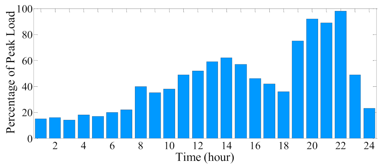
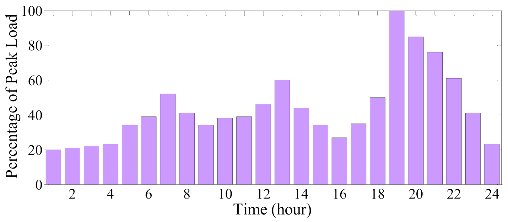
2.1. Microgrid’s Demand

The contemplated microgrid is a local distribution network that has a variable load during a day. With regard to the incremental trend of consumption of residential and industrial loads at the early hours of the evening, the peak of the demand curve is supposed to be in the evening. In addition, with regard to the consumption pattern of industrial loads, another peak exists around midday hours. Thus, in order to consider the load pattern of the microgrid, a 24 h load profile with two peaks is taken into account as figured out as follows. Figure 1 demonstrates the normalized demand of the microgrid. It is noteworthy to assert that the load of the distribution network is also determined in a similar way.

2.2. Microgrid’s Supply Strategy

The first goal of size determination of microgrid’s generation sources is to supply the loads in this micro-scale grid. The PV panels have a vital role in power provision for the loads. However, when PV panels cannot generate sufficient power, the energy storage unit and diesel generator unit are responsible for meeting the loads. Thus, the optimal supply strategy can be express as follows:

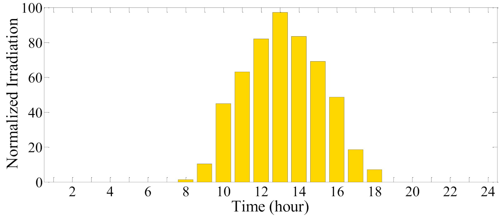
2.2.1. Enjoying Photovoltaic Panel’s Power

• If the PV generation is more than the grid’s demand and the batteries are not fully charged, the excess PV generation should be stored in the batteries;
• If the PV generation is more than the grid’s demand and the batteries are fully charged, the excess generation of PV panels must be sold to the distribution network;
• If the PV generation is lower than the grid’s demand, a portion of the loads will be supplied through PV generation, and the rest of the demand must be procured through the energy storage system;
• If the PV generation is lower than the grid’s demand and the battery system is not adequate to supply the loads entirely, the loads will be satisfied by PV panels and energy storage units as much as possible, and the rest of the loads must be met by the diesel generator;
• If the total generation by PV panels, batteries, and the diesel generator is not sufficient for satisfying the load, the load-shedding measure must be imposed for the excessive demand.

2.2.2. Being Deprived of PV Generation

• If the batteries’ capacity is adequate to supply the demand, the loads will be served by the batteries solely;
• If the batteries’ capacity is not sufficient to supply the demand, the rest of the loads must be served by the diesel generator;
• If the demand is more than the combined capacity of PV panels and the diesel generator, the rest of the loads must be remained unsupplied by load shedding.

It should be noted that the unsupplied load cannot be higher than 25% of the total demand of the grid. In addition, the capacity of the diesel generator must be so determined that it is not allowed to operate less than 20% of its maximum capable generation.

2.3. The Objective Function

When the suggested capacities for the generation sources are adequate to supply the microgrid’s loads properly, the excess generated power can be sold to the distribution network. However, it must be determined which bus in the distribution network must be chosen, from which the excess generation will be injected into the distribution grid. The injection point has a considerable impact on the performance of the distribution grid. Thus, the location of the microgrid is an important item. Hence, the optimal placement of the microgrid must be investigated. The objective function for the optimal placement of the microgrid can be expressed as follows:

$$\min f=C_{PV}+C_{loss}+C_{bat}+C_{dg}-B_{ex}$$

(1)

2.3.1. Power Losses

In order to model the power losses, the losses are supposed to be as a power, which must be bought from the upstream network. Thus, it is modeled as a cost in the overall objective function equation. This objective can be expressed as follows:

$$C_{loss}={\displaystyle \sum _{d=1}^{365}{\displaystyle \sum _{t=1}^{24}{\displaystyle \sum _{i=1}^{N_b}{P}_{{}_{loss}}^{i,t,d}\times {\rho }^{t,d}}}}$$

(2)

In the above equation, ρ^t,d denotes the price of electricity on the day of d at hour t, and $P_{loss}^{i,t,d}$ stands for the number of losses on the day of d at hour t in the ith line. It is noticeable that the price of electricity at peak, mid-peak, and off-peak hours is different.

2.3.2. The Cost Related to the Photovoltaic System

Deployment of solar energy incurs installation cost of PV panels, operation and maintenance cost, and replacement cost. Thus, the cost pertaining to PV panels can be modeled as below. The subscript of PV a is a symbol for a photovoltaic unit, O&M addresses operation and maintenance cost, inv indicates investment cost, and rep corresponds with replacement cost.

$$C_{PV}=C_{PV\_inv}+C_{PV\_O\&M}+C_{PV\_rep}$$

(3)

2.3.3. The Battery Cost

The energy storage facility in this work is a set of batteries that have similar costs, such as the PV panel, and can be formulated as Equation (4). The subscript of bat stands for battery energy storage system, O&M addresses operation and maintenance cost, inv indicates investment cost, and rep corresponds with replacement cost.

$$C_{bat}=C_{bat\_inv}+C_{bat\_O\&M}+C_{bat\_rep}$$

(4)

2.3.4. The Cost Pertaining to Diesel Generator

The cost of such equipment consists of investment cost, maintenance cost, and replacement cost. The subscript of dg stands for the diesel generator, O&M addresses operation and maintenance cost, inv indicates investment cost, and rep corresponds with replacement cost.

$$C_{dg}=C_{dg\_inv}+C_{dg\_O\&M}+C_{dg\_rep}$$

(5)

2.3.5. The Cost Pertaining to Load Shedding

If the load-shedding measure has to be imposed, this matter incurs a cost to the model, which must be included in the objective function of the problem.

2.3.6. The Profit Yielded by Excess Generation Selling

If the power generated by the PV panel is higher than the demand of the microgrid and charging capability of batteries, the excess power can be sold to the distribution network and earn a profit. The obtainable benefit (profit) can be calculated by the following equation:

$$B_{ex}={\displaystyle \sum _{d=1}^{365}{\displaystyle \sum _{t=1}^{24}{P}_{{}_{ex}}^{t,d}\times {\rho }^{t,d}}}$$

(6)

In above, B_ex is the benefit (profit) gain by the sale of surplus generation, and $P_{ex}^{t,d}$ shows the amount of surplus power on the day of d and at hour t.

2.3.7. Constraints

The optimization problem is accompanied by a set of technical constraints that restrict the solution space and must be considered in the model. These constraints can be defined as follows:

The power balance equality constraint during all intervals of a day:

$${\displaystyle \sum _{t=1}^{24}{P}_{PV}^t+P_{dg}^t+P_{bat}^t-P_{D\_mic}^t}=0$$

(7)

The maximum permissible load shedding in the microgrid:

$${\displaystyle \sum _{t=1}^{24}{P}_{sh}^t}\le 0.25\times {\displaystyle \sum _{t=1}^{24}{P}_{D\_mic}^t}$$

(8)

Generation balance in the distribution network must be observed.

$${\displaystyle \sum _{t=1}^{24}{P}_g^t+P_{ex}^t+P_{slack}^t-P_{loss}^t-P_{D\_dis}^t}=0$$

(9)

The boundaries of the photovoltaic panel and diesel generator must be met.

$$0<P_{PV}<P_{PV}^{\max }$$

(10)

$$0<P_{dg}<P_{dg}^{\max }$$

(11)

The voltage of buses must be restricted within their permissible range.

$$V_{\min }<V<V_{\max }$$

(12)

The power flow passing through the lines must be restricted.

$$F_b<Limi{t}_b$$

(13)

In the above equations, $P_{PV}^t$, $P_{dg}^t$, and $P_{bat}^t$ represent power generation of PV panel, diesel generator, and batteries, respectively. Moreover, $P_{D\_mic}^t$ indicates the consumption of the microgrid at hour t. The shed load of the microgrid is shown by $P_{sh}^t$. In addition, $P_g^t$, $P_{ex}^t, P_{slack}^t$, $P_{loss}^t$, and $P_{D\_dis}^t$ represent the power generated by the generators in the distribution network, the exchanged power of the microgrid with the distribution network, the power maintains from the slack bus of the distribution network, the power losses in the distribution network, and the consumption of the distribution network at hour t. Moreover, $P_{PV}^t$, $P_{dg}^t$, V, V_min, V_max, F_b, and Limit_b stand for the maximum capable power generation by PV panel, the maximum capable power generation by a diesel generator, bus voltage, the minimum and maximum permissible voltage of buses, the flow passing through branch b, and the thermal limit of branch b.

The prevailing constraints of the problem can be divided into two general categories of network constraints and storage constraints that must always be observed when seeking for optimal point in the solution space. Network constraints include the following two constraints:

As the thermal limit constraints express, the feeder power flow is not allowed to violate a specific cap.

$$S_k\le \lim i{t}_k$$

(14)

The hourly constraints pertaining to the energy storage unit consist of two constraints of the maximum storage capacity and charge/discharge rate limits. This limitation expresses that the storage charge level must always be below the maximum storage capacity and can be formulated as follows:

$$P_{min\_ch}^{}\times I_{ch}(t)\le P_{ch}^{}\left(t\right)\le P_{max\_ch}^{}\times I_{ch}(t)$$

(15)

$$P_{min\_dch}^{}\times I_{dch}(t)\le P_{dch}^{}\left(t\right)\le P_{max\_dch}^{}\times I_{dch}(t)$$

(16)

$$So{C}_{min}^{}\le SoC\left(t\right) \le So{C}_{max}^{}$$

(17)

$$SoC\left(t+1\right)=SoC\left(t\right)-P_{dch}\left(t\right)\times I_{dch}\left(t\right)+P_{ch}\left(t\right)\times I_{ch}\left(t\right)$$

(18)

$$I_{ch}(t)+I_{sch}(t)\le 1$$

(19)

In this equation, t represents the time, P_ch and P_dch denote the charge and discharge rates, and SoC stands for the state of charge of the storage unit that has a maximum storage capacity limit and a minimum storage capacity boundary owing to the long-run operation and maintenance facets. Each storage unit can be charged or discharged by a limited amount within an hour. The last equation also ensures that the storage unit cannot operate at charge and discharging modes simultaneously. In this equation, I(t) is a binary variable.

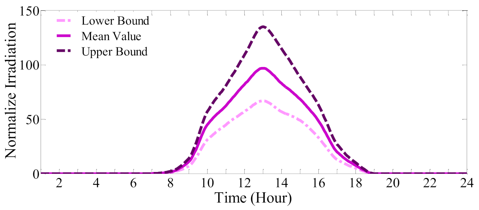
2.3.8. The Uncertainty Modeling for PV Sources

The nature of solar power and photovoltaic irradiance can be represented by various types of distribution functions. One of the most efficient types for this purpose is the lognormal probability distribution function (PDF), which effectively and precisely characterizes the intensity of irradiance on a typical day. The PDF of solar irradiance (ζ_s) trailing the lognormal distribution function with a mean value of μ_s and standard deviation of σ_s that is presented in Equation (20).

$$f\left({\zeta }_s|{\mu }_s,{\sigma }_s^2\right)=\frac{1}{{\sigma }_s^2\sqrt{2\pi }}\exp \left\{-\left(\frac{{\left(\log \left({\zeta }_s\right)-{\mu }_s\right)}^2}{2{\sigma }_s^2}\right)\right\} \forall {\zeta }_s>0$$

(20)

The solar power generation (P_PV) depends on the solar radiation intensity, also known as solar irradiance, which is shown by ζ_s. The generation curve can be different based on different items such as the location and type of installation, the technology of solar panels, as well as the ambient temperature. A typical photovoltaic irradiance-power curve is given in Equation (21).

$$P_{PV}^{}\left({\zeta }_s\right)=A_{PV}{\eta }_{pv}{\zeta }_s$$

(21)

$${\eta }_{pv}={\eta }_0[1-0.0042 (\frac{{\zeta }_s}{18}+T_a-20)] {\eta }_{\mathrm{inv}}$$

(22)

The amount of power generation by a solar panel depends on different factors, which can be estimated by Equations (21) and (22). Above, η stands for efficiency, and T_a denotes the ambient temperature.

In order to model the intermittencies, a dataset of historical records associated with the solar radiation. Such irradiance datasets can effectively be matched with a lognormal or Weibull distribution function. These distribution models usually have high mathematical compatibility with various natural phenomena. The PDF helps to generate randomly derived samples within the occurrence range while specifying a confidence range to eliminate low-probable cases. For each scenario, a random value is derived from the lognormal model. If the number of scenarios is high, various scenario reduction techniques can be employed that merge similar cases into one class. Based on the model objectives, the operation state can be adjusted within the confidence range with respect to the level of risk chosen by the operator. The operator can arrange the operation point in a risk-averse zone to ensure a reliable and secure operation, although it incurs higher costs. On the other hand, the operation of the grid, with respect to the whole uncertainties, can be stated in a high-risk zone by ignoring less-probable incidences to boost the profitability and the economy of the model.

2.3.9. Load Forecast Uncertainty

Load forecasting is a critical item in many planning applications in power systems. Load forecasting can also be performed in different intervals for various purposes. Load forecasts are dependent on weather conditions (temperature, humidity, air brightness, wind speed). In addition, each day of the week has its own load curve. Load consumption curves on holidays and non-holidays are also different from each other. In different seasons of the year, according to the factors specific to each season, such as day length, the load consumption pattern will be different. Short-term load forecasting is a pivotal data needed for running a day-ahead market. The results of STLF are employed by GENCOs to discover prices with regard to the way other market participants may act. Price forecast signals are also applied to bidding strategy techniques to maximize profitability. The system operator will clear the market for the next-day delivery according to the forecasted values along with the bids from GENCOs. ISO is responsible for balancing the market between generation level and the forecasted demand at each interval. However, with regard to the inaccuracy of forecasts, there is always a violation that must be redressed by storage units or other controlling actions such as load shedding.

There are multiple approaches to deal with load forecasting. The most common methods are the time series method, regression methods, and intelligent methods. Intelligent methods are also classified into several categories such as artificial neural networks, fuzzy logic-based methods, also ANFIS models, wavelet transformation methods, as well as support vector machines. In order to deal with uncertainties, probabilistic models can be integrated into the employed load forecasting paradigm. In this study, the Gaussian process quantile regression (GPQR) is employed to deal with uncertainties [38]. Due to the stochastic nature of load patterns as well as various external factors such as weather conditions, calendar effects, and seasonal factors, the power demand signals exhibit intermittent and volatile characteristics. Hence, a prediction scheme is needed to provide the most probable distribution of power demand patterns rather than a crisp value. A Gaussian process model is a set of random variables, in which any member corresponds with a probability distribution that can be represented by the following function:

$$f\left(l\right)\sim GP\left(\mu \left(l\right),COV\left(l,l^{\prime }\right)\right)$$

(23)

In this equation, μ(l) and COV(l,l′) denote the mean and covariance functions that can be calculated as follows:

$$\mu \left(l\right)=E\left\{f\left(l\right)\right\}$$

(24)

$$COV\left(l,l^{\prime }\right)=E\left\{\left[f\left(l\right)-\mu \left(l\right)\right]\times {\left[f\left(l^{\prime }\right)-\mu \left(l^{\prime }\right)\right]}^T\right\}$$

(25)

The covariance function illustrates the similarity between data points. One of the most widely-used functions for describing covariance is the squared exponential (SE) model that can be represented as follows:

$$CO{V}_{SE}\left(l,l^{\prime }\right)={\theta }_f^2\exp \left(\frac{‖l-l^{\prime }‖}{{\theta }_{length}^2}\right)$$

(26)

The parameters θ_f and θ_l control the scale and length. With regard to the differentiability of this covariance, which implies that the Gaussian process is very smooth, a simplified alternative, known as Matern covariance, can be replaced because, in practice, no phenomena do not reflect such a strong smoothness.

$$CO{V}_{Mat}\left(l-l^{\prime }\right)={\sigma }^2\frac{2^{1-v}}{\mathrm{\Gamma }\left(v\right)}{\left(\sqrt{2v}\frac{l-l^{\prime }}{i}\right)}^v{B}_v\left(\sqrt{2v}\frac{l-l^{\prime }}{i}\right)$$

(27)

In the above, B_v represents the modified Bessel function, in which v and i are both positive hyperparameters. To simplify this covariance function, the value of v is supposed to be v = p + 1/2. In this parameter, p is a non-negative integer. The value of v is set as 5/2 or 3/2 in most previously conducted research studies, which subsequently and, respectively, are named Mat5 and Mat3. The probabilistic prediction model also has another covariance function named the period covariance, which is useful to model periodic phenomena and can be described as follows:

$$CO{V}_{Mat}\left(l,l^{\prime }\right)={\theta }_f^2\exp \left(-\frac{2}{{\theta }_{length}^2}{\sin }^2\left(\pi \frac{l-l^{\prime }}{p}\right)\right)$$

(28)

Typically, the load forecasts are highly influenced by a variety of features that can be defined by Equation (29). According to this equation, load at time t depends on the similar hours (t∈{0, 24}) throughout the historical records, the day of the year (d∈{1, …, 365}), the value of the load at similar intervals, the value of weather variables such as temperature, and the price at similar intervals.

$$\widehat{y}=f\left(t,d,v_l,v_w,price\right)$$

(29)

GPQR method seeks for the relationships and correlation between inputs and output based on a probabilistic framework. Quantile regression (QR) delineates a type of regression analysis that detects and exploits the relationships between quantiles of the conditional distribution of a response variable and input variables. The least absolute deviations regression integrates the median of the conditional distribution, which is called the norm regression case of quantile regression shown by L₁. Unlike least-squares regression and norm regression, the quantile regression encompasses minimization of the summation of asymmetrically weighted absolute residuals. Hence, QR can find more sophisticated relationships between inputs and outputs with better precision. QR has more flexibility and compatibility to deal with large datasets, such as market analysis or econometrics. With regard to the accuracy of predictions, the loss function can be described as follows:

$$L_{\tau }\left({\epsilon }_i\right)=\left\{\begin{array}{lllllll}\tau {\epsilon }_i& & & if& & & {\epsilon }_i\ge 0\\ \left(\tau -1\right){\epsilon }_i& & & if& & & {\epsilon }_i\ge 0\end{array}\right.$$

(30)

The required quantile is defined by τ∈[0, 1] and ${\epsilon }_i=y_i-{\widehat{y}}_i$ so that y_i is the actual model and ${\widehat{y}}_i$ denotes the predicted quantile model. So far, different linear programming methods are employed to achieve the desired quantiles through direct loss function minimization, which leads to the maximization of a likelihood. To solve this drawback, the Gaussian process is incorporated into the QR model. The density function of loss based on this model can be represented as follows:

$$L\left(t|\mu ,\sigma ,\tau \right)=\frac{\tau \left(1-\tau \right)}{\sigma }\exp \left[-\frac{t-\mu }{\sigma }\left(t-I\left(t\le \mu \right)\right)\right]$$

(31)

where τ∈[0, 1] is responsible for shaping and controlling the skewness of the distribution curve, μ stands for the mean value, and σ denotes the standard deviation, which should always be positive. The binary variable I takes the value of 1 when the condition is true; otherwise, it takes 0.

$$U_{\tau }\left(y,q\right)=Z\exp \left[-{\displaystyle \sum _{i=1}^N{L}_{\tau }\left(y_i,q_i\right)}\right]$$

(32)

In Equation (32), q denotes the predicted value of the τ quantile, Z is the normalization constant. Afterward, a Gaussian process is placed on the QR function:

$$p\left(q\right)=GP\left(q|0,K\right)$$

(33)

The GPQR model training can be conducted by integral maximization. The expectation propagation algorithm can be employed to locally approximate this integral.

$$\arg \max \underset{q}{\mathsf{\int }}{U}_{\tau }\left(y,q\right)p\left(q\right) d\left(q\right)$$

(34)

Suppose a dataset of historical load records as l = {x₁, x₂, …, x_N}, which are independently distributed samples. The estimated shape of this distribution function can be obtained through a Gaussian kernel density estimator model.

$$K\left(x_1,x_2,\sigma \right)=\frac{1}{\sqrt{2\pi }\sigma }{e}^{-\frac{{\left(x_1-x_2\right)}^2}{2{\sigma }^2}}$$

(35)

Mean absolute percentage errors (MAPE) and root mean squared error (RMSE) are two employed evaluation metrics that can exhibit the performance of the forecasting model.

$$RMSE\left(y_i,{\widehat{y}}_i\right)=\sqrt{\frac{1}{N}{\displaystyle \sum _{i=1}^N{\left(y_i,{\widehat{y}}_i\right)}^2}}$$

(36)

$$MAPE\left(y_i,{\widehat{y}}_i\right)=\frac{1}{N}{\displaystyle \sum _{i=1}^N\left|\frac{y_i,{\widehat{y}}_i}{y_i}\right|}$$

(37)

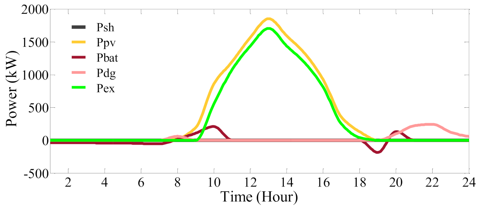
2.4. Energy Management Paradigm by Microgrid’s Controller

The controlling framework of a microgrid is a vital element in this planning scheme. The microgrid controller, also known as the microgrid operator, is responsible for collecting raw data and analyzing them to find the optimum operation point with respect to all operational constraints of both sides. In other words, it has to provide an accurate estimation of generation sources for all intervals and take a sensible range of risk for being preserved from the detrimental zone. Then it can dedicate the level of power exchange with the upstream grid for various hours. To implement such an intelligent autonomous mechanism, a smart environment is needed that is only feasible through IoT infrastructures [39]. The following flowchart concisely describes the proposed scheme. The paradigm of the proposed scheme is depicted in Figure 2.

3. Lightning Attachment Procedure Optimization (LAPO) Method

This algorithm was inspired by the procedure of lightning the attachment process to the ground or any type of earthed object. In order to simulate this optimization algorithm, at first, some test points are considered on a cloud or the ground as the initial population. By increasing the electric field at the points on the cloud, the streamer channels begin to break down the air and move toward the ground, which is called a downward leader. As these downward leaders move toward the ground, the opposite charges will be enhanced in the ground and produce upward leaders. The striking point at the final jump step is a point where the upward leader collides with the downward leader [40,41,42]. The algorithm is composed of some sections that will be presented as follows:

3.1. Initialization

At first, the test points on the surface of a cloud as well as on the ground are defined. These dedicated charges are called the initial population.

3.2. The Next Jumping Node

Each branch of the lightning has some probable points in front of itself, which can move toward one of them. The choice of the next jumping point of the lightning is highly correlated with the intensity of the electric field between the point and the probable points. Of course, the next jump will not necessarily be toward the point with the maximum field, and part of the process of selecting the next point will occur randomly. For the mathematical modeling of this section, a random node is selected for each node in the search space. If the electric field in this point (merit value of the point or the fitness value at the intended point) is greater than the background field (which is supposed to be the mean field), the lightning moves toward this point; otherwise, the path of lightning will be in another direction. It is noticeable that the term opposite direction does not imply an upward movement exclusively rather than an angled motion toward this point. Hence, for determining the next jump, the following equation can be employed:

$$P=sign(F_{av}-F(r))$$

(38)

$$X_{new}(i,j)=X(i,j)-P\times rand\times (Xav(1,j)-X(r,j))$$

(39)

3.3. Streaming Forward and Elimination of Branches

When a new lightning branch is formed, this branch can stream downward until the branch’s charge cuts down and becomes lower than a specific value (critical value). The critical value is assigned to be 1 μC because the air cannot be broken down for the lower levels of charges, and the branch will be faded.

3.4. Upward Leader Propagation

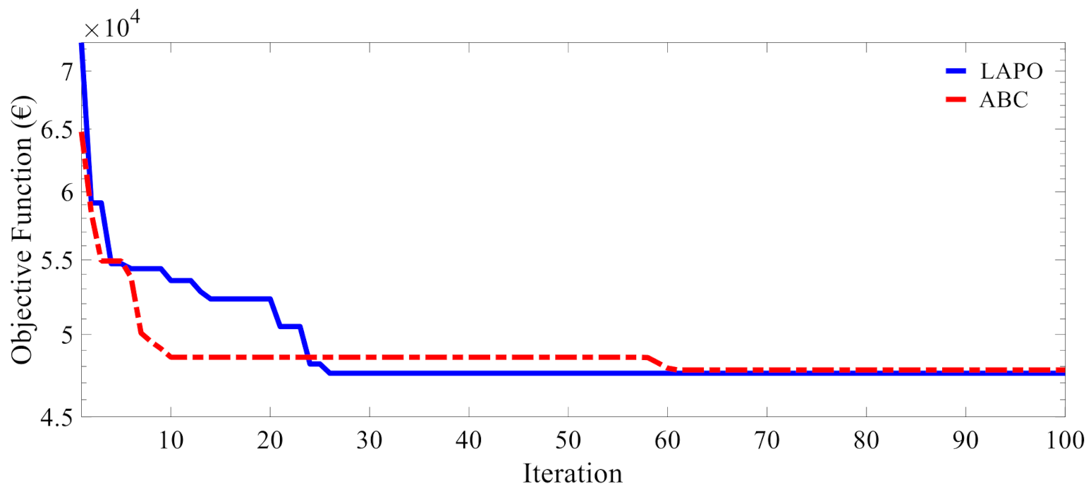
When the branches start to move downward, the upward leaders start to move upward. The motion speed of the upward leader is correlated with the amount of charge aggregated at this point as well as the total charge of the downward branch. The distribution of charge in the downward branch is so that there are fewer charges near the cloud and more charge at the tip of the leader. This is why the tip of the leader is brighter. This incremental charge aggregation over the branch can be considered as a linear or exponential function. Here, the branch’s charge is considered exponentially, as pointed out by the following two equations:

$$S=1-\left(t/t_{\max }\right)\times \exp \left(-t/t_{\max }\right)$$

(40)

$$Cc=S\times (X_{\min }(i,j)-X_{\max }(i,j))$$

(41)

Above, C_C denotes the branch’s charge, X_min is the charge of the branch in the tip of the leader, X_max indicates the branch’s charge at the beginning point. The upward leaders will be propagated according to the following equation:

$$X_{new}(i,j)=X(i,j)+rand\times Cc$$

(42)

3.5. Convergence

When an upward leader reaches a downward leader, the collision point of the lightning will be determined. In other words, when the optimum point is specified, the algorithm will be terminated. The abovementioned procedure will be iteratively executed until the optimum point is found.

4. Simulation and Results

In this section, the optimal placement for the microgrid is carried out on the targeted test system. The targeted system is a radial 69-bus IEEE test system, which is depicted in Figure 3 in the form of a single-line diagram. In addition, in order to have a better appraisal of the effectiveness of the proposed method, the proposed method is also tested on a radial 33-bus IEEE test system, which is depicted in Figure 4. However, the input data is the same for both grids. In this paper, all the methods are implemented in MATLAB 2018a in a Core i5 PC with 3 GHz processing frequency of CPU and 8 GB of RAM. The convergence behavior is another aspect with which the methods are compared to each other.

The characteristics corresponded with the lines and the buses of this system refer to [43,44], respectively. The normalized demand of the microgrid is shown in Figure 5. The demand for this microgrid at the peak is considered to be 250 kW. The peak of the load curve of the grid is supposed to be the mid-peak demand obtained from [43,44]. Moreover, the hourly solar insulation profile is normalized and illustrated in Figure 6.

The maximum generation capability of the PV panel per month is shown in

Table 1. The mean solar radiation for each month for both radiation systems. [45].

Jan.	Feb.	Mar.	Apr.	May	Jun.	Jul.	Aug.	Sep.	Oct.	Nov.	Dec.
5.45	5.73	6	6.01	5.65	5.26	4.81	4.78	5.15	5.63	5.84	5.57

. The placement mechanism is executed in the worst condition. Thus, the calculations are conducted for the month of August. This month indicates the lowest level of mean solar radiation.

The economic data for different sources were extracted from reference [44]. The investment cost of the PV panel is considered to be 7.44 €/kW, and the O&M cost is supposed to be 40 €/year. The cost of each battery is determined as 0.283 €/Ah, and each battery incurs 50 €/year for O&M costs. The operation cost and maintenance cost of the diesel generator is 0.55 €/W and 0.2 €/h, respectively.

The demand in the targeted microgrid is supposed to be composed of residential and industrial loads.

Table 2. The electricity price for different load types and various demand levels for both distribution systems.

Load Level	Price of Residential Load (€/MW)	Price of Industrial Load (€/MW)	Percent of Peak Load
Low	35	2000	50 < L
Middle	49	2800	50 < L < 70
Peak	70	3050	L > 70

delineates the price of electricity corresponded with the types of loads and the demand level.

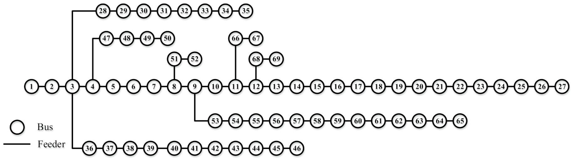
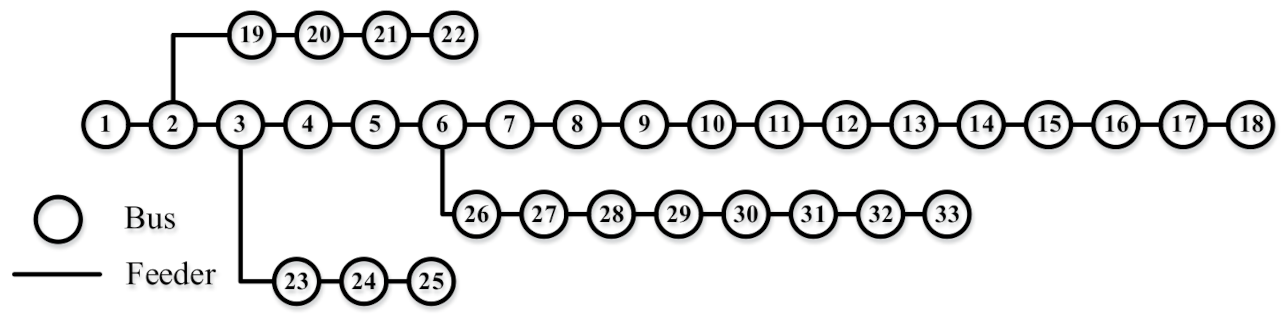
4.1. The IEEE Test Systems (33-Bus and 69-Bus)

The optimization for the 33-bus test network is conducted with regard to the acquired economic data. The results are demonstrated in

Table 3. The design and size determination of microgrid for the distribution test systems (33-bus and 69-bus).

Bus	Method	Location	PV Size (Kw)	Diesel Size (Kw)	Number of Batteries	Cost (€)
33	LAPO	6	395	242	25	47,162
	ABC	26	393	242	25	47,383
69	LAPO	59	400	256	26	50,360
	ABC	61	399	238	25	52,351

. In addition, the convergence behavior of two targeted methods in reaching the optimal solution is illustrated in Figure 7. Accordingly, the LAPO method has reached the optimal solution with fewer iteration. In terms of accuracy, the results of LAPO are better than the ABC algorithm. As can be seen, at the early hours of the time horizon (at midnight), when there is no solar power generation, a battery energy storage unit can supply the demand of internal loads of the microgrid as it is clear that the battery power is negative during these hours, which indicates that it is discharged. The battery starts charging after 8:00 and reaches its maximum charge level at 11:00. Therefore, no power is stored in it until it starts discharging again at 18:00. It is recharged at 19:00 and fully discharged at 20:00 due to the high volume of consumption. The diesel generator commits at 8:00 and stops power exchange at 9:00. These conditions continue until 20:00, and after that, it continues to serve the loads until midnight. Due to the significant amount of solar production, a large volume of this production is sold to the distribution network, and the obtained profit improves the objective function. As it is evident, the network is designed in such a way that no load is interrupted during the day and all the loads are completely satisfied.

With regard to the economic data provided in the previous section, the optimization problem is simulated on the 69-bus test system. The optimized results of the simulation are presented in Table 3. In addition, the convergence behavior of both optimization techniques employed in this study is depicted in Figure 8. As can be seen, it is evident that the LAPO approach not only has reached the optimal solution in less iteration, but also it has found a better solution in comparison with the ABC method.

The behavior of the microgrid in August is illustrated in Figure 9. As can be perceived, in the early hours at midnight, while the sunrise has not occurred, the battery is responsible for maintaining power for the microgrid. Thus, the power battery is negative in these hours, which implies that the battery is discharging. The battery starts to be charged at 8:00 in the morning, and it will be fully charged at 11:00. Hence, the batteries will not be charged anymore and remain idle until 18:00. At 18:00, the batteries are to some extent discharged. However, they are charged again at 19:00. With regard to the high level of consumption at 20:00, the batteries deliver all of their stored energy to the microgrid. The diesel generator is connected to the microgrid at 8:00, and it is disconnected at 9:00. It continues until 19:00. Again, at 19:00, the diesel generator starts to supply the load until the end of the time horizon of this study (24:00). With respect to the high level of solar generation, a considerable share of this production is sold to the distribution grid. The obtained economic benefit has improved the objective function. As it is clear, the microgrid is so designed that the loads are supplied entirely and load shedding has not occurred. The microgrid behavior in August is depicted in Figure 9.

The power purchased from the main grid is shown in Figure 7. As it shows, during the day hours when there is solar energy, the demanded power from the upstream grid is drastically reduced. It should also be noted that the network losses and the corresponding costs were 1061 kW and 55.86 € per day, which reached the values of 956.79 kW and 51.78 € per day, after the installation of microgrids in the network, respectively. Figure 8 shows the amount of load shedding in the distribution network at different times of the day. The results figure out that during the hours when there is solar energy, solar unit injects power into the distribution network, the amount of shed load has reached zero, which is very beneficial in terms of cost and efficiency for the distribution network as well as reliability improvement from microgrid point of view. The model is also tested on the 69-bus test system. The results imply that the bought power from the main grid by the 69-bus distribution network is illustrated in Figure 10. As it is evident, during the hours that the PV panel can generate power, the absorbed power from the sub-transmission grid is considerably diminished. The power losses of the distribution grid and the subsequent cost of them were about 1350 kW equivalent with 65.76 €/day before the implementation of the microgrid scheme, and it is alleviated to 989.32 and 56.28 €/day after implementation of the microgrid. In Figure 11, the hourly shed load in the distribution network is shown. It is obvious that whenever the PV generation exists, all of the loads in the distribution grid are satisfied, and no load-shedding measure in the distribution network is executed. This matter significantly improves the performance of the distribution network.

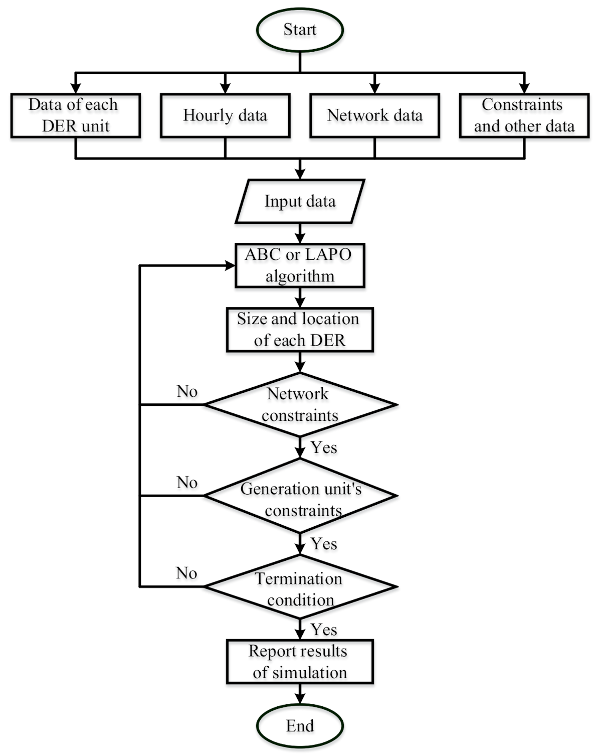
4.2. Incorporation of Uncertainty in the Model

The demand for a grid and the daily radiation intensity are not deterministic parameters, and they usually have uncertainties. Hence, these parameters must be forecasted, and the scheduling must be conducted based on the forecasts. Therefore, the existence of forecasting error is inevitable, and the error must be included in the optimization model in order to mitigate the risk. A common way to model the uncertainties corresponded with solar radiation and demand of the grid is to employ a normal probability distribution. In other words, the mean value and the standard deviation of these parameters are calculated, and the design and the scheduling must be carried out based on these forecasts.

The most famous and the most accurate approach for dealing with uncertainties and probabilistic problems is the Monte Carlo algorithm. In this approach, a large number of probabilistic samples are defined within a specified range, and the scheduling is performed for all of these samples. Then, the probability density function of targeted parameters is extracted. In this study, an upper and a lower boundary are dedicated for the demand of microgrid and distribution network along with the daily solar radiation. It is supposed that the radiation and demand will be materialized within the defined range. These boundaries are depicted in Figure 12, Figure 13, and Figure 14.

In order to solve the stochastic problem, the Monte Carlo approach is employed. In this respect, for each uncertain parameter, 1000 stochastic samples are generated randomly. To solve the stochastic problem, the following step-by-step procedure is considered:

• Step 1—Generation of 1000 samples for each uncertain optimization variable.
• Step 2—The stochastic generation of a set of solutions for optimization variables.
• Step 3—The selection of a set of optimization variables.
• Step 4—Test the grid’s performance for 1000 samples using the Monte Carlo approach and checking all constraints for 1000 plausible scenarios.
• Step 5—The calculation of the objective function (if the constraints are met).
• Step 6—Check convergence and termination conditions. If it is converged, then go to step 9.
• Step 7—The change of optimization variables based on the optimization method.
• Step 8—Go to step 3.
• Step 9—End.

Table 4. The results of optimal sizing of test grids incorporating uncertainties of demand and solar radiation and the consideration of the maximum cost of stochastic scenarios as the objective function.

Bus	Location	PV Size	Diesel Size	Number of Batteries	Cost (€)
33	2	395	215	42	70,342
69	6	400	214	39	69,214

outlines the results of the design of the microgrid with the incorporation of uncertainties.

In the case of the 33-bus test system, the cost of power generation is greatly increased. This increase is due to the conditions in which the load may be maximum and production may be minimum. Therefore, these conditions must also be taken into account in the problem. However, as can be seen, the cost has increased by nearly 49% compared to the case where uncertainty is not considered. Thus, it should be considered that in the presence of sources of intermittency, the cost of power supply from the network may increase remarkably, which conveys the importance of stochastic solution.

The increase in the system cost pertaining to the uncertainty will be 27%, which is nearly 20% less than the previous case. Therefore, the uncertainties are applied to the model using the average intermittencies in the system cost in all possible scenarios as an objective function. As can be seen, in the stochastic model, the cost of the system has increased by 26% compared to the deterministic case.

As the results of the 69-bus test system figure out, the cost of supply in this condition is significantly increased. This increase conveys a condition that the demand is at a high level and the solar radiation is at a low level. Therefore, the worst conditions must be contemplated in the design of the microgrid. However, as it is evident, the cost is drastically increased by 50% in comparison with the case of the deterministic model (regardless of uncertainties). Thus, it should be noted that the overall cost of the microgrid scheme may be enhanced extensively for uncertain problems.

It is important to pay attention to a critical question. The cost of supply has increased by 50% in order to include uncertainties. It conveys a high level of consumption and a low level of generation. The occurrence of such generation and consumption levels for this system at the targeted time is not a definitive and certain event. The question is whether it is sensible to increase the cost of the system by 50% for a forecast that has an occurrence probability of 10%.

In the procedure of seeking the optimum solution of uncertain parameters, for each suggested answer provided by the optimization program, all possible scenarios are taken into account, and the highest cost incurred to the system, among all scenarios, is regarded as the cost of the suggested answer. If the suggested answer does not satisfy even one or more constraints, that answer should be dismissed. Such a procedure profoundly mounts the system cost.

In order to tackle this problem, no answer should be dismissed, and the system cost must be obtained for all answers in as scenarios, even when they were unable to meet some constraints. Finally, the average cost of all scenarios is dedicated to the answer. Hence, if the suggested answer does not meet the constraints in some scenarios, the answer will not be dismissed. It is obvious that, for the problems with a few scenarios, the inclusion of scenarios, which used to be disregarded, does not have a remarkable impact on the solution of the problem. With consideration of the proposed condition, the optimal results of the simulation can be expressed in

Table 5. The results of optimal sizing of test grids incorporating uncertainties of demand and solar radiation and the consideration of the average cost of stochastic scenarios as the objective function.

Bus	Location	PV Size	Diesel Size	Number of Batteries	Cost (€)
33	2	395	253	37	59,802
69	2	400	265	34	59,325

. This assumption has been led to an increase of 26% in the system cost for the incorporation of uncertainties in the model. It is just over 20% fewer than the normal approach. Thus, the uncertainties can be included in the design by incorporation of the average cost of the system. As can be seen, the system cost has increased by 26% in comparison with the deterministic approach.

5. Conclusions

In this study, a microgrid scheme including loads, PV panels, energy storage system, and the backup supply system of a diesel generator was designed. The object of the design was to minimize the cost of supply. In this microgrid, it was intended to not absorb any power from the distribution grid. However, if there is an excess of generation by intrinsic power resources of the microgrid, the excess power would be sold to the distribution network. The costs pertaining to PV panels, batteries, and diesel generator consists of purchasing and installation cost, operation and maintenance cost, and replacement cost. If the proposed scheme cannot supply the loads (generation deficiency) at some hours, the load-shedding measure must be imposed for the surplus demand. Just the same, the excess generation must be injected into the upstream network. In order to boost the performance of the design, the placement of the microgrid is so determined that the network power losses are minimized. Thus, the optimal design of the microgrid was performed at the same time as the placement of the microgrid. The problem solution was targeted to be stochastic. Hence, two upper and lower boundaries were dedicated to the amount of demand and solar irradiance. In order to solve the problem, the Monte Carlo approach with 6222 random samples is employed. The results of the 33-bus test system imply that the incorporation of uncertainties in the model has drastically increased the supply cost by about 49%. In order to avoid unnecessary risks, the averaging method is deployed, which boosts the risk-averse scheduling. In this case, the system cost has increased by 27% in comparison with the deterministic approach. The results of the 69-bus test system imply that the incorporation of uncertainties in the model has drastically increased the supply cost by about 50%. In order to avoid unnecessary risks, the averaging method is deployed, which boosts the risk-averse scheduling. In this case, the system cost has increased by 26% in comparison with the deterministic approach. The optimization is solved using the LAPO method, and the results are compared with the ABC algorithm. The results indicate the proper performance of the suggested algorithm in terms of convergence speed and accuracy.

References

1. Gil-González, W.; Garces, A.; Montoya, O.D.; Hernández, J.C. A Mixed-Integer Convex Model for the Optimal Placement and Sizing of Distributed Generators in Power Distribution Networks. Appl. Sci. 2021, 11, 627. [Google Scholar] [CrossRef]
2. Nafisi, H.; Agah, S.M.M.; Abyaneh, H.A.; Abedi, M. Two-Stage Optimization Method for Energy Loss Minimization in Microgrid Based on Smart Power Management Scheme of PHEVs. IEEE Trans. Smart Grid 2015, 7, 1268–1276. [Google Scholar] [CrossRef]
3. Nafisi, H.; Farahani, V.; Abyaneh, H.A.; Abedi, M. Optimal daily scheduling of reconfiguration based on mini-misation of the cost of energy losses and switching operations in microgrids. IET Gener. Transm. Distrib. 2015, 9, 513–522. [Google Scholar] [CrossRef]
4. Hosseini, S.J.A.D.; Moradian, M.; Shahinzadeh, H.; Ahmadi, S. Optimal Placement of Distributed Generators with Regard to Reliability Assessment using Virus Colony Search Algorithm. Int. J. Renew. Energy Res. 2018, 8, 714–723. [Google Scholar]
5. Hamzeh, M.; Vahidi, B.; Nematollahi, A.F. Optimizing Configuration of Cyber Network Considering Graph Theory Structure and Teaching-Learning-Based Optimization (GT-TLBO). IEEE Trans. Ind. Inform. 2018, 15, 2083–2090. [Google Scholar] [CrossRef]
6. Thatte, A.A.; Xie, L. Towards a Unified Operational Value Index of Energy Storage in Smart Grid Environment. IEEE Trans. Smart Grid 2012, 3, 1418–1426. [Google Scholar] [CrossRef]
7. Das, T.; Krishnan, V.; McCalley, J.D. Assessing the benefits and economics of bulk energy storage technologies in the power grid. Appl. Energy 2015, 139, 104–118. [Google Scholar] [CrossRef]
8. Rahiminejad, A.; Aranizadeh, A.; Vahidi, B. Simultaneous distributed generation and capacitor placement and sizing in radial distribution system considering reactive power market. J. Renew. Sustain. Energy 2014, 6, 43124. [Google Scholar] [CrossRef]
9. Moazzami, M.; Gharehpetian, G.B.; Shahinzadeh, H.; Hosseinian, S.H. Optimal locating and sizing of DG and D-STATCOM using Modified Shuffled Frog Leaping Algorithm. In Proceedings of the 2017 2nd Conference on Swarm Intelligence and Evolutionary Computation (CSIEC), Kerman, Iran, 7–9 March 2017; Institute of Electrical and Electronics Engineers (IEEE): Piscataway, NJ, USA, 2017; pp. 54–59. [Google Scholar]
10. Karunarathne, E.; Pasupuleti, J.; Ekanayake, J.; Almeida, D. Optimal Placement and Sizing of DGs in Distribution Networks Using MLPSO Algorithm. Energies 2020, 13, 6185. [Google Scholar] [CrossRef]
11. Cho, B.; Ryu, K.; Park, J.; Moon, W.; Cho, S.; Kim, J. A Selecting Method of Optimal Load on Time Varying Distribution System for Network Reconfiguration considering DG. J. Int. Counc. Electr. Eng. 2012, 2, 166–170. [Google Scholar] [CrossRef]
12. Aman, M.; Jasmon, G.; Bakar, A.; Mokhlis, H. A new approach for optimum simultaneous multi-DG distributed generation Units placement and sizing based on maximization of system loadability using HPSO (hybrid particle swarm optimization) algorithm. Energy 2014, 66, 202–215. [Google Scholar] [CrossRef]
13. Ameli, A.; Bahrami, S.; Khazaeli, F.; Haghifam, M.-R. A multiobjective particle swarm optimization for sizing and placement of DGs from DG owner’s and distribution company’s viewpoints. IEEE Trans. Power Deliv. 2014, 29, 1831–1840. [Google Scholar] [CrossRef]
14. Buaklee, W.; Hongesombut, K. Optimal DG Placement in a Smart Distribution Grid Considering Economic As-pects. J. Electr. Eng. Technol. 2014, 9, 1240–1247. [Google Scholar] [CrossRef] [Green Version]
15. Wang, Z.; Chen, B.; Wang, J.; Kim, J.; Begovic, M.M. Robust Optimization Based Optimal DG Placement in Microgrids. IEEE Trans. Smart Grid 2014, 5, 2173–2182. [Google Scholar] [CrossRef]
16. Alotaibi, M.; Almutairi, A.; Salama, M. Effect of wind turbine parameters on optimal DG placement in power dis-tribution systems. In Proceedings of the 2016 IEEE Electrical Power and Energy Conference (EPEC), Ottawa, ON, Canada, 12–14 October 2016; Institute of Electrical and Electronics Engineers (IEEE): Piscataway, NJ, USA, 2016. [Google Scholar]
17. Hengsritawat, V.; Tayjasanant, T.; Nimpitiwan, N. Optimal sizing of photovoltaic distributed generators in a dis-tribution system with consideration of solar radiation and harmonic distortion. Int. J. Electr. Power Energy Syst. 2012, 39, 36–47. [Google Scholar] [CrossRef]
18. Carpentiero, V.; Langella, R.; Testa, A. Hybrid wind-diesel stand-alone system sizing accounting for component expected life and fuel price uncertainty. Electr. Power Syst. Res. 2012, 88, 69–77. [Google Scholar] [CrossRef]
19. Hakimi, S.M.; Moghaddas-Tafreshi, S.M. Optimal sizing of a stand-alone hybrid power system via particle swarm optimization for Kahnouj area in south-east of Iran. Renew. Energy 2009, 34, 1855–1862. [Google Scholar] [CrossRef]
20. Ma, T.; Yang, H.; Lu, L. A feasibility study of a stand-alone hybrid solar-wind-battery system for a remote island. Appl. Energy 2014, 121, 149–158. [Google Scholar] [CrossRef]
21. Hassan, A.S.; Sun, Y.; Wang, Z. Multi-objective for optimal placement and sizing DG units in reducing loss of power and enhancing voltage profile using BPSO-SLFA. Energy Rep. 2020, 6, 1581–1589. [Google Scholar] [CrossRef]
22. Reddy, P.D.P.; Reddy, V.V.; Manohar, T.G. Ant Lion optimization algorithm for optimal sizing of renewable energy resources for loss reduction in distribution systems. J. Electr. Syst. Inf. Technol. 2018, 5, 663–680. [Google Scholar] [CrossRef]
23. Alzahrani, A.; Alharthi, H.; Khalid, M. Minimization of power losses through optimal battery placement in a dis-tributed network with high penetration of photovoltaics. Energies 2020, 13, 140. [Google Scholar]
24. Farh, H.M.H.; Al-Shaalan, A.M.; Eltamaly, A.M.; Al-Shamma’A, A.A. A Novel Crow Search Algorithm Auto-Drive PSO for Optimal Allocation and Sizing of Renewable Distributed Generation. IEEE Access 2020, 8, 27807–27820. [Google Scholar] [CrossRef]
25. HassanzadehFard, H.; Jalilian, A. Optimal sizing and location of renewable energy based DG units in distribution systems considering load growth. Int. J. Electr. Power Energy Syst. 2018, 101, 356–370. [Google Scholar] [CrossRef]
26. Hemeida, M.G.; Ibrahim, A.A.; Mohamed, A.-A.A.; Alkhalaf, S.; El-Dine, A.M.B. Optimal allocation of distributed generators DG based Manta Ray Foraging Optimization algorithm (MRFO). Ain Shams Eng. J. 2021, 12, 609–619. [Google Scholar] [CrossRef]
27. Jalili, A.; Taheri, B. Optimal Sizing and Sitting of Distributed Generations in Power Distribution Networks Using Firefly Algorithm. Technol. Econ. Smart Grids Sustain. Energy 2020, 5, 1–14. [Google Scholar] [CrossRef] [Green Version]
28. Lata, P.; Vadhera, S. Optimal placement and sizing of energy storage systems to improve the reliability of hybrid power distribution network with renewable energy sources. J. Stat. Manag. Syst. 2020, 23, 17–31. [Google Scholar] [CrossRef]
29. Mukhopadhyay, B.; Das, D. Multi-objective dynamic and static reconfiguration with optimized allocation of PV-DG and battery energy storage system. Renew. Sustain. Energy Rev. 2020, 124, 109777. [Google Scholar] [CrossRef]
30. Shahinzadeh, H.; Moradi, J.; Gharehpetian, G.B.; Nafisi, H.; Abedi, M. IoT Architecture for Smart Grids. In Proceedings of the 2019 International Conference on Protection and Automation of Power System (IPAPS), Tehran, Iran, 8–9 January 2019; Institute of Electrical and Electronics Engineers (IEEE): Piscataway, NJ, USA, 2019; pp. 22–30. [Google Scholar]
31. Shahinzadeh, H.; Moradi, J.; Gharehpetian, G.B.; Nafisi, H.; Abedi, M. Internet of Energy (IoE) in Smart Power Systems. In Proceedings of the 2019 5th Conference on Knowledge Based Engineering and Innovation (KBEI), Tehran, Iran, 28–29 February 2019; Institute of Electrical and Electronics Engineers (IEEE): Piscataway, NJ, USA, 2019; pp. 627–636. [Google Scholar]
32. Ebeed, M.; Ali, A.; Mosaad, M.I.; Kamel, S. An Improved Lightning Attachment Procedure Optimizer for Optimal Reactive Power Dispatch With Uncertainty in Renewable Energy Resources. IEEE Access 2020, 8, 168721–168731. [Google Scholar] [CrossRef]
33. Youssef, H.; Kamel, S.; Ebeed, M. Optimal Power Flow Considering Loading Margin Stability Using Lightning Attachment Optimization Technique. In Proceedings of the 2018 Twentieth International Middle East Power Systems Conference (MEPCON, Nasr City, Egypt, 18–20 December 2018; Institute of Electrical and Electronics Engineers (IEEE): Piscataway, NJ, USA, 2018; pp. 1053–1058. [Google Scholar]
34. Ramadan, A.; Ebeed, M.; Kamel, S.; Nasrat, L. Optimal Allocation of Renewable Energy Resources Considering Uncertainty in Load Demand and Generation. In Proceedings of the 2019 IEEE Conference on Power Electronics and Renewable Energy (CPERE), Aswan, Egypt, 23–25 October 2019; Institute of Electrical and Electronics Engineers (IEEE): Piscataway, NJ, USA, 2019; pp. 124–128. [Google Scholar]
35. Ebeed, M.; Alhejji, A.; Kamel, S.; Jurado, F. Solving the Optimal Reactive Power Dispatch Using Marine Predators Algorithm Considering the Uncertainties in Load and Wind-Solar Generation Systems. Energies 2020, 13, 4316. [Google Scholar] [CrossRef]
36. Ramadan, A.; Ebeed, M.; Kamel, S.; Nasrat, L. Optimal power flow for distribution systems with uncertainty. In Uncertainties in Modern Power Systems; Elsevier BV: Amsterdam, The Netherlands, 2021; pp. 145–162. [Google Scholar]
37. Ebeed, M.; Aleem, S.H.E.A. Overview of uncertainties in modern power systems: Uncertainty models and methods. In Uncertainties in Modern Power Systems; Elsevier BV: Amsterdam, The Netherlands, 2021; pp. 1–34. [Google Scholar]
38. Yang, Y.; Li, S.; Li, W.; Qu, M. Power load probability density forecasting using Gaussian process quantile regres-sion. Appl. Energy 2018, 213, 499–509. [Google Scholar] [CrossRef]
39. Sirat, A.P.; Mehdipourpicha, H.; Zendehdel, N.; Mozafari, H. Sizing and Allocation of Distributed Energy Resources for Loss Reduction using Heuristic Algorithms. In Proceedings of the 2020 IEEE Power and Energy Conference at Illinois (PECI), Champaign, IL, USA, 20–21 February 2020; Institute of Electrical and Electronics Engineers (IEEE): Piscataway, NJ, USA, 2020; pp. 1–6. [Google Scholar]
40. Nematollahi, A.F.; Rahiminejad, A.; Vahidi, B. A novel physical based meta-heuristic optimization method known as Lightning Attachment Procedure Optimization. Appl. Soft Comput. 2017, 59, 596–621. [Google Scholar] [CrossRef]
41. Nematollahi, A.F.; Rahiminejad, A.; Vahidi, B.; Askarian, H.; Safaei, A. A new evolutionary-analytical two-step optimization method for optimal wind turbine allocation considering maximum capacity. J. Renew. Sustain. Energy 2018, 10, 043312. [Google Scholar] [CrossRef]
42. Nematollahi, A.F.; Rahiminejad, A.; Vahidi, B. A novel multi-objective optimization algorithm based on Lightning Attachment Procedure Optimization algorithm. Appl. Soft Comput. 2019, 75, 404–427. [Google Scholar] [CrossRef]
43. Nematollahi, A.F.; Dadkhah, A.; Gashteroodkhani, O.A.; Vahidi, B. Optimal sizing and siting of DGs for loss reduction using an iterative-analytical method. J. Renew. Sustain. Energy 2016, 8, 055301. [Google Scholar] [CrossRef]
44. El-Zonkoly, A. Optimal placement of multi-distributed generation units including different load models using particle swarm optimization. Swarm Evol. Comput. 2011, 1, 50–59. [Google Scholar] [CrossRef]
45. El-Zonkoly, A. Optimal placement and schedule of multiple grid connected hybrid energy systems. Int. J. Electr. Power Energy Syst. 2014, 61, 239–247. [Google Scholar] [CrossRef]
Figure 1. The normalized demand curve of the microgrid.
Applsci 11 04156 g001
Figure 2. The paradigm of the proposed scheme.
Applsci 11 04156 g002
Figure 3. The single-line diagram of the 69-bus test system.
Applsci 11 04156 g003
Figure 4. The single-line diagram of the 33-bus test system.
Applsci 11 04156 g004
Figure 5. The normalized demand of distribution network for both systems.
Applsci 11 04156 g005
Figure 6. The normalized daily solar irradiance for both distribution systems.
Applsci 11 04156 g006
Figure 7. The comparison of the convergence behavior of different methods in seeking for the best solution for the 33-bus distribution test system.
Applsci 11 04156 g007
Figure 8. The comparison of the convergence behavior of different methods in seeking for the best solution for the 69-bus distribution test system.
Applsci 11 04156 g008
Figure 9. The behavior of the microgrid in August.
Applsci 11 04156 g009
Figure 10. The bought power from the main power system by the distribution network.
Applsci 11 04156 g010
Figure 11. The amount of shed load in the distribution network in the presence and absence of microgrid.
Applsci 11 04156 g011
Figure 12. The upper bound, the lower bound, and the mean value of demand of microgrid in the probabilistic study.
Applsci 11 04156 g012
Figure 13. The upper bound, the lower bound, and the mean value of demand of distribution network in the probabilistic study.
Applsci 11 04156 g013
Figure 14. The upper bound, the lower bound, and the mean value of daily solar irradiance in the probabilistic study.
Applsci 11 04156 g014