Abstract
A systematic device-model calibration (extraction) methodology has been proposed to reduce parameter calibration time of advanced compact model for modern nano-scale semiconductor devices. The adaptive pattern search algorithm is a variant of the direct search method, which explore in the parameter space with adaptive searching step and direction. It is very straightforward, but powerful, in high dimensional optimization problem since adaptive step and direction are decided by simple computation. The proposed method iterates less but shows superior accuracy over the conventional method. It is possible to be applied to a behavioral or empirical model correspond to emerging devices, such as tunneling field-effect transistor (TFET) and negative capacitance field-effect transistor (NCFET) due to its universality in parameter calibration for the model accuracy.
1. Introduction
As the dimension of the silicon transistor shrink in size, their development period is prolonged due to complex fabrication processes. To be competitive in the foundry business, the accuracy and agility of the model-device fitting process is crucial in evaluating chip-level functional verification and performance estimation during the early development stage. In the modern compact model, several hundreds of parameters are used to capture the DC and AC characteristics of nano-scale transistor. It is not practical to calibrate these parameters manually for all fabricated transistors.
Levenberg–Marquardt (LM) method [1,2,3] and genetic algorithm (GA) [4,5,6,7,8,9] have been proposed to automate model parameter calibration (extraction). However, the LM method tends to be stuck into local optimum without proper initial guess. GA is a global optimizer for combinatorial optimization problem which is not desirable to continuous parameter tuning.
The pattern search algorithm is one of the direct searching algorithms [10,11,12]. This method is a very simple and fast local searching algorithm since it is derivative-free and depends only on simple calculation. It is capable of stepping over the hillocks in the parameter space to escape from local optima due to the independence on derivation in the pattern vector. However, it loses information to a certain extent in high dimensional problem since it does not utilize any information gained in the pattern move. In this paper, an adaptive pattern search algorithm is proposed to calibrate the parameters systematically with enhanced model accuracy and reduced calibration time.
2. Problem Definition
The compact model is computationally efficient description of the terminal properties of the electrical devices, such as diode, bipolar junction transistor and metal-oxide-semiconductor field-effect transistor (MOSFET) to simulate the behavior of VLSI system [13,14,15,16,17,18,19,20,21]. Restricting the direct current property, a simple mathematical representation of the compact model is as follows:
where the vector and are the terminal voltage biases, and parameters of the model, respectively, and the is the simulated drain current vector from the compact model, corresponding to bias conditions. Calibrating (extracting) the compact model parameter means adjusting the set of parameters to fit the simulation data derived from the model to measurement data of the transistor. The objective of parameter calibration is:
to minimize the mean of squared relative error (MSRE), a fitness function, between simulated and measured values, where ID is the measured drain current, which is the target output vector for the optimization. MSRE is used as a fitness function, rather than MSE, due to the wide dynamic range of the drain current.
Usually, model parameters for the given device are calibrated by the experts manually. Therefore, it is very tedious and time-consuming work and hard to deal with massive number of devices fabricated for the development of the new technology. A systematic extraction of model parameter is to find optimal algorithm to optimize the fitness of the model rapidly with practically low computational cost.
3. Configuration of the Experiment
In this paper, we focus on the Berkeley Short-channel Insulated-gate field-effect transistor Model 4 (BSIM4) [13,14,15,16] as a base model to be calibrated by proposed algorithm. It seems to be well enough to utilize BSIM4 to test our methodology since it is a physics based compact model and considered as an industry standard [16]. Target current vectors, in this study, are generated from the given model using commercial circuit simulator. The type and the physical parameters of the device for the target data is N channel MOSFET and length/width = 0.1 μm/1 μm, respectively. Each target current vector is simulated with random value of the model parameters. Each parameter’s value is uniformly sample in the certain range that handles the on current (@VG = 1.5 V, VD = 1.5 V) from 5~10% reduction to 5~10% increase. The parameter list and the specification we handle for the experiment is summarized in Table 1. Although, we verify the algorithm with BSIM4, a general approach in calibrating the parameters involves fitting the model and target, thus, it can apply to any kind of compact model, such as BSIM Common Multi-Gate (BSIM-CMG) [17,18], Enz-Krummenacher-Vittoz (EKV) [19], Pennsylvania State university and Philips (PSP) [20,21] and any kind of behavioral and empirical model composed of analytical equation and parameters. Also, it is possible to calibrate the models to describe emerging devices, such as TFET, NCFET and Feedback FET.

Table 1.
The list of parameters and specification for the experiment. Lower and upper bound is set up to keep the physical meaning up in the optimization process. The number format for the boundary is the engineering format. The type and the physical parameters for the experiment is N channel MOSFET and length/width = 0.1 μm/1 μm, respectively. The value in the parentheses follows by bound value of parameter is the relative variation of the on current by parameter change at the bound compared to the reference, BSIM4′s default parameter.
4. Pattern Search Algorithm
Pattern search algorithm is a kind of direct search algorithm widely adopted in the field of optimization. By default, the pattern search is a local optimizer, but it has the characteristics of a global optimizer [10,11]. Unlike the ‘Newtonian method’ based algorithms, it does not rely on the gradient so that it can deviate from local optimum. Therefore, a pattern search algorithm can be applied to optimize the problems on non-continuous and non-differentiable searches. The best-known pattern search algorithm is originated by Hooke-Jeeves (HJ) method could be utilized either way as a non-constrained and constrained optimization problem [10,11]. For the compact model parameter calibration (extraction), model parameters should be constrained within the specific boundary to keep the physical meaning of the model. Therefore, we set up the algorithm as a constrained optimization problem for the given parameter space to find the point that minimizes the fitness value between the given target current vector and simulated current vector.
The method consists of two main processes, so-called exploratory move and pattern move. At first, the initial point, which is the basis of this study, is uniformly sampled from the parameter space. In an exploratory move, the algorithm evaluates the two neighboring points around the exploration basis in all axes and takes the best point among them. Unlike the gradient based algorithm, fixed length of step size is used for exploration in each dimension. In each axis of parameter space, ternary exploration, thus, +step size, 0 or –step size displacements are added to exploration basis and evaluated at that points to pick the displacement for the axis. Then, the ternary exploration is performed on the following axis from the new exploration basis decided in previous step. This sequential exploration is adopted in the HJ method to reduce the exploration time and computational cost. A displacement between the final point and the exploration basis is set to the direction vector to be used in the following process.
In the pattern move, the algorithm evaluates the points where the direction vector reaches until the fitness is no longer improving. In other words, the pattern move is the naïve line search algorithm on one dimensional parameter space that loosely minimizes the fitness. The one-dimensional parameter space is projected from original multi-dimensional parameter space along the direction vector. After reaching the loosely minimized point, then algorithm set the point to exploration basis and repeats the two processes again until a magnitude of the displacement vector is less than 1e-9, thus, it is at no better point than basis is found. To optimize further, exploration range, so called step size, is reduced by scale factor (SF) and repeat the whole process again. The algorithm is terminated when it meets termination criteria, such as target fitness and minimum step size. Lower bound of fitness value is set to 1e-8 as a target. Since a step size of exploration that is too small is meaningless, a minimum step size is set to 1e-6, as the main termination criterion of the whole process, as well as the fitness target. A detailed interpretation and process flow chart is shown in Figure 1 and Figure 2.
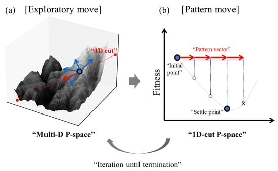
Figure 1.
The graphical conceptualization of the exploratory move and pattern move of patter search algorithm: (a) Exploratory move. In the multi-dimensional parameter space, adjacent points around the exploration basis (blue dot surrounded by black line) are evaluated in the process and the displacement between best point and the exploration basis is set to pattern vector (red arrow). 1-dimensional projection along the pattern vector will be the stage for the following process; (b) Pattern move. One-dimensional naïve line search is performed with the given pattern vector. The process is terminated when the newest point is not improved more then set the previous point to be the next exploration basis (settle point).
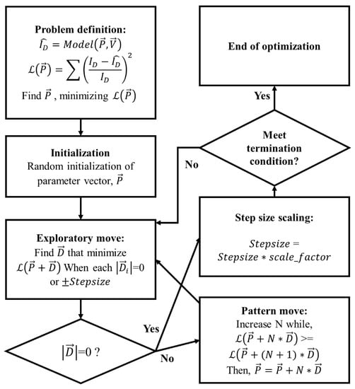
Figure 2.
Flow chart of an original construction of Hooke-Jeeves method. is the target current vector measured from fabricated MOSFET and is the relative mean-squared error served as a fitness function. In exploratory move, the algorithm evaluates the adjacent points around the exploration basis in all axes and takes the best point among them. In the pattern move, the algorithm evaluates the points where the direction vector reaches until the fitness is no longer improving.
5. Results
5.1. Adaptive Pattern Search
5.1.1. Adaptive Pattern Move
For the pattern move defined as in the conventional HJ method, searching basis moves forward to searching direction by constant step [10,11]. This is simple and uses no other computation, except for the evaluation of the point reached. However, it is too naïve and cannot utilize the information gained spontaneously during pattern move, such as the trajectory of losses and momentum, which can assist the process in figuring out the shape of parameter space. In the case of very small magnitude of the pattern vector, it often travels in the low slope region unnecessarily and takes lots of iterations in the pattern move (Red arrows in the Figure 3a). If the magnitude of the pattern vector increases as the slope of the valley decreases, it can pass through gradual region much faster than constant pattern vector and reduce the iterations of the pattern move (Blue arrows in the Figure 3a). On the contrary, if the magnitude of pattern vector is too large to sample the loss valley properly, it just hops over the hillocks in the parameter space and misunderstands the underlying shape of the valley (Red arrows in the Figure 3b). As the rough sampling with constant pattern vector, it misjudges as it explores the gradual valley. If the magnitude of pattern vector is varied with respect to the information of the parameter space, it has a chance to fumble around and figure out the underlying geometry. In the toy model described in Figure 3b, it settles in the first valley as intended owing to the adaptive pattern move (Blue arrows in the Figure 3b). In this study, the normalized differences in fitness values between the two neighboring points is utilized in the pattern move to scale the searching step adaptively. As the patter vector advances, it is inversely scaled by the normalized difference of losses between the points. The implementation of adaptive pattern move is depicted in Figure 3c.
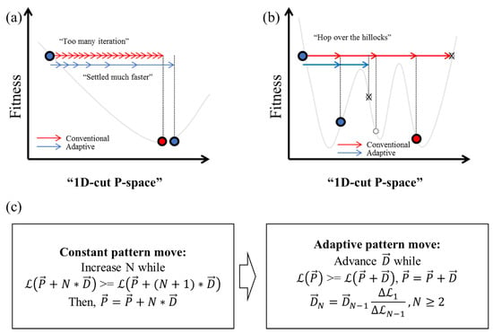
Figure 3.
(a) The graphical interpretation of pattern move when the pattern vector is relatively small and fitness valley has a gradual slope. Red arrow represents the pattern vector of the conventional method and blue arrow represents the adaptive pattern vector. Unnecessary iteration of evaluations and advances is needed with this circumstance with the constant vector. Scaling the pattern vector adaptively, pattern move can be settled much faster; (b) the graphical interpretation of pattern move when the pattern vector is relatively large and fitness valley has a steep slope. In this circumstance, the algorithm could not capture the underlying structure of fitness valley and leads to wrong conclusion. Along with the adaptive pattern vector, this misleading vector can be reduced; (c) the mathematical description of adaptive pattern move. Constant pattern of conventional method is revised to vary adaptively utilizing the relative difference of fitness to scale the pattern vector.
For the benchmark of the adaptive pattern move and conventional implementation, iteration count of exploratory moves and pattern moves, and the fitness value of the calibrated parameters for 10 samples are represented in Figure 4. Exploration count retains the same degree, while pattern move count has reduced by 74% in the worst case and 49% in the median. In terms of fitness, MSRE has reduced by 25% in the worst case and 1% in the median. The variation of fitness values is also reduced compared to the conventional method. Along with the adaptively varying searching step, searching process converges faster and more accurate compared to conventional method owing to the variety of information used in the process.
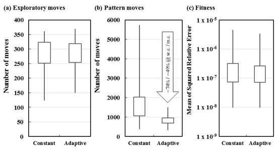
Figure 4.
The benchmark results of adaptive pattern move and constant pattern move in the HJ method. To be fair in comparison, 10 samples of the target curves are randomly chosen and used on both implementations. The scale factor = 0.1 is configured in this benchmark. (a) The number of moves in exploratory move; (b) The number of moves in pattern move; (c) fitness distribution of the calibrated parameters; w.c. refers to worst case and m.c. refers to median case. A top/bottom edge of the whisker in the plot represents the maximum/minimum datum, respectively.
5.1.2. Parallel Exploration
In an exploratory move, conventional HJ method explores (2Md + 1) number of points sequentially to decide searching direction, when Md is the number of dimensionalities, thus the length of parameter vector. It evaluates the ternary displacement −1, 0, +1 with the scale of searching step in each dimension independently and chooses the best displacement compared to the exploration basis (0 displacements for all dimension) [10,11]. The number of all possible directions with ternary displacement is the 3 to the power of Md. In a high dimensional problem, conventional exploratory move explores only a part of possible directions, so it compromises accuracy to computational cost. However, evaluations in each direction can be fully parallelized with many-core machine, or even utilizes the thousands of cores in graphical processing unit. Along with the parallel implementation of evaluation, parallel exploration is substantially advantageous in sequential exploration since it leads the pattern move to the best direction among all possible choices in the ternary exploration. This is conceptualized in Figure 5.
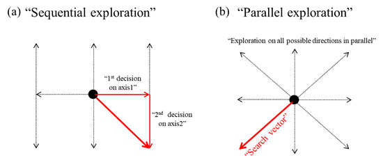
Figure 5.
(a) The concept of sequential exploration. In each axis of parameter space, ternary exploration, thus +step size, 0 or −step size from the exploration basis (black dot) is performed and decide the direction for the axis. Then same process is performed on the following axis. (b) The concept of parallel exploration. The all-possible directions in the ternary exploration are evaluated in parallel at the same time and find the best direction among them.
Comparisons carried out between sequential exploration and parallel exploration is depicted in Figure 6. In terms of the parallel exploration, the number of moves both in the exploratory and the pattern move has improved. The number of exploration move is reduced by 7% in worst case and 86% in the median case by the parallel exploration, and the number of pattern moves is reduced by 89% in worst case and 97% in the median. The parallel exploration prevents the misjudgment of the direction in the exploratory move and makes the process converges much quicker than sequential one. Also, preventing the misleading to bad local optima, the fitness of the calibration is enhanced by 99% in worst case and 93% in median case. In short, parallel exploration with full searching in the direction enhances the searching time and fitness utilizing the parallelization of evaluation.
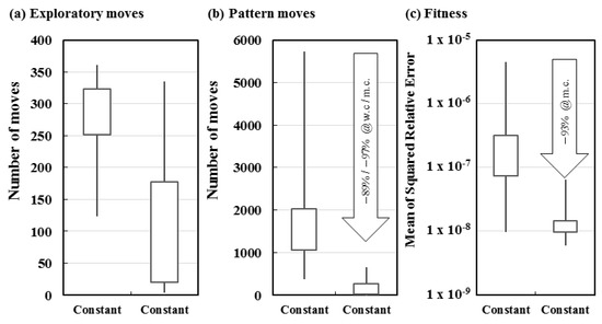
Figure 6.
The benchmark results of sequential exploration and parallel exploration. To be fair in comparison, 10 samples of the target curves are randomly chosen and used on both implementations. The scale factor = 0.1 is configured in this benchmark. (a) The number of moves in exploratory move; (b) the number of moves in pattern move; (c) fitness distribution of the calibrated parameters; w.c. refers to worst case and m.c. refers to median case. A top/bottom edge of the whisker in the plot represents the maximum/minimum datum, respectively.
5.2. Curve Fitting Result
For the verification of the proposed method, drain current and trans-conductance, a first derivative of drain current with respect to gate voltage, from the calibrated parameters and target data are compared in the Figure 7, Figure 8 and Figure 9 with respect to the progress of the optimization process. At first, simulated curves are not matched with the target curve at all. As the optimization progresses, simulated curves become matched with the target curves. In relation to the calibrated parameters, all ranges of data points are well fitted with target curves.
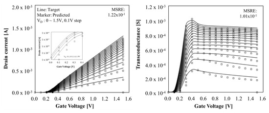
Figure 7.
Comparison between simulated curves with the initial parameters and the target curves. The type and the physical parameters for the experiment is N channel MOSFET and length/width = 0.1 μm/1 μm, respectively. Line denotes the target curves and marker denotes the calibrated model curves. (a) Transfer curves of the N channel MOSFET, inset shows the sub-threshold region in log-scale; (b) Transconductance of the N channel MOSFET.
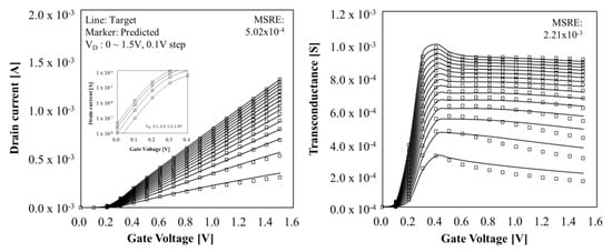
Figure 8.
The curve fitting results of the calibrated parameters after 100 iterations by adaptive pattern search. The type and the physical parameters for the experiment is N channel MOSFET and length/width = 0.1 μm/1 μm, respectively. Line denotes the target curves and marker denotes the calibrated model curves. (a) Transfer curves of the N channel MOSFET, inset shows the sub-threshold region in log-scale; (b) Transconductance of the N channel MOSFET.

Figure 9.
The curve fitting results of the calibrated parameters after optimization is finished by adaptive pattern search. The type and the physical parameters for the experiment is N channel MOSFET and length/width = 0.1 μm/1 μm, respectively. Line denotes the target curves and marker denotes the calibrated model curves. (a) Transfer curves of the N channel MOSFET, inset shows the sub-threshold region in log-scale; (b) Trans-conductance of the N channel MOSFET.
6. Discussion
In this work, a systematic calibration methodology of compact model parameters based on adaptive pattern search algorithm is demonstrated. Utilizing the information gained in the pattern move process and parallel exploration, we found that the proposed algorithm is superior to the conventional approach, in terms of accuracy and computational cost and time. The proposed method accurately calibrates the model to target data with optimized configuration. The proposed algorithm is a general approach to calibrate the model parameters, so it can be applied to any kind of models, even for the emerging devices. For the future work, we will expand the methodology and apply to the models for the emerging devices.
Author Contributions
Conceptualization, J.C., S.H., K.-K.M., M.-H.O. and T.J.; methodology, J.C., software, K.P. and J.P.; writing—original draft preparation, J.C.; writing—review and editing, J.C. and B.-G.P.; supervision, B.-G.P. and J.-H.L.; project administration, B.-G.P. All authors have read and agreed to the published version of the manuscript.
Funding
This work was supported by the BK21 FOUR program of the Education and Research Program for Future ICT Pioneers, Seoul National University in 2020 and in part by Institute of Information and communications Technology Planning and Evaluation (IITP) grant funded by the Korea government (MSIT) (No. 2020-0-01294, Development of IoT based edge computing ultra-low power artificial intelligent processor).
Institutional Review Board Statement
Not applicable.
Informed Consent Statement
Informed consent was obtained from all subjects involved in the study.
Data Availability Statement
Not applicable.
Conflicts of Interest
The authors declare no conflict of interest.
References
- Levenberg, K. A method for the solution of certain non-linear problems in least squares. Q. Appl. Math. 1944, 2, 164–168. [Google Scholar] [CrossRef]
- Marquardt, D.W. An Algorithm for Least-Squares Estimation of Nonlinear Parameters. J. Soc. Ind. Appl. Math. 1963, 11, 431–441. [Google Scholar] [CrossRef]
- Singh, K.; Jain, P. BSIM3v3 to EKV2.6 Model Parameter Extraction and Optimisation Using LM Algorithm on 0.18 Micron Technology Node. Int. J. Electon. Telecommun. 2018, 64, 5–11. [Google Scholar]
- Goldberg, D.E. Genetic Algorithms in Search, Optimization and Machine Learning, 13th ed.; Addison-Wesley Professional: Reading, MA, USA, 1988; ISBN 978-0-201-15767-3. [Google Scholar]
- Karr, C.; Weck, B.; Massart, D.; Vankeerberghen, P. Least median squares curve fitting using a genetic algorithm. Eng. Appl. Artif. Intell. 1995, 8, 177–189. [Google Scholar] [CrossRef]
- Fogel, D.B. Evolutionary Computation: The Fossil Record, 1st ed.; Wiley-IEEE Press: New York, NY, USA, 1998; ISBN 978-0-7803-3481-6. [Google Scholar]
- Jervase, J.A.; Bourdoucen, H.; Al-Lawati, A. Solar cell parameter extraction using genetic algorithms. Meas. Sci. Technol. 2001, 12, 1922–1925. [Google Scholar] [CrossRef]
- Spałek, T.; Pietrzyk, P.; Sojka, Z. Application of the Genetic Algorithm Joint with the Powell Method to Nonlinear Least-Squares Fitting of Powder EPR Spectra. J. Chem. Inf. Model. 2005, 45, 18–29. [Google Scholar] [CrossRef] [PubMed]
- Li, Y. An automatic parameter extraction technique for advanced CMOS device modeling using genetic algorithm. Microelectron. Eng. 2007, 84, 260–272. [Google Scholar] [CrossRef]
- Hooke, R.; Jeeves, T.A. “Direct Search’’ Solution of Numerical and Statistical Problems. J. ACM 1961, 8, 212–229. [Google Scholar] [CrossRef]
- Torczon, V. On the Convergence of Pattern Search Algorithms. SIAM J. Optim. 1997, 7, 1–25. [Google Scholar] [CrossRef]
- Ayala-Mató, F.; Seuret-Jiménez, D.; Escobedo-Alatorre, J.J.; Vigil-Galán, O.; Courel, M. A hybrid method for solar cell parameter estimation. J. Renew. Sustain. Energy 2017, 9, 063504. [Google Scholar] [CrossRef]
- Parke, S.; Moon, J.; Wann, H.; Ko, P.; Hu, C. Design for suppression of gate-induced drain leakage in LDD MOSFETs using a quasi-two-dimensional analytical model. IEEE Trans. Electron Devices 1992, 39, 1694–1703. [Google Scholar] [CrossRef]
- Liu, Z.H.; Hu, C.; Huang, J.H.; Chan, T.Y.; Jeng, M.C.; Ko, P.; Cheng, Y. Threshold voltage model for deep-submicrometer MOSFETs. IEEE Trans. Electron Devices 1993, 40, 86–95. [Google Scholar] [CrossRef]
- Hu, C. BSIM4.8.1 MOSFET MODEL Users Manual; UC Berkeley: Berkeley, CA, USA, 2017. [Google Scholar]
- Cheng, Y.; Hu, C. MOSFET Modeling & BSIM3 User’s Guide; Springer: New York, NY, USA, 2002; ISBN 978-0-7923-8575-2. [Google Scholar]
- Venugopalan, S.; Lu, D.D.; Kawakami, Y.; Lee, P.M.; Niknejad, A.M.; Hu, C. BSIM-CG: A compact model of cylindrical/surround gate MOSFET for circuit simulations. Solid State Electron. 2012, 67, 79–89. [Google Scholar] [CrossRef]
- Khandelwal, S.; Duarte, J.P.; Chauhan, Y.S.; Hu, C. Modeling 20-nm Germanium FinFET With the Industry Standard FinFET Model. IEEE Electron Device Lett. 2014, 35, 711–713. [Google Scholar] [CrossRef]
- Enz, C.C.; Vittoz, E.A. An analytical MOS transistor model valid in all regions of operation and dedicated to low-voltage and low-current applications. Analog. Integr. Circuits Signal Process. 1995, 8, 83–114. [Google Scholar] [CrossRef]
- Gildenblat, G.; Li, X.; Wu, W.; Wang, H.; Jha, A.; Van Langevelde, R.; Smit, G.; Scholten, A.; Klaassen, D. PSP: An Advanced Surface-Potential-Based MOSFET Model for Circuit Simulation. IEEE Trans. Electron Devices 2006, 53, 1979–1993. [Google Scholar] [CrossRef]
- Li, X.; Wu, W.; Jha, A.; Gildenblat, G.; Van Langevelde, R.; Smit, G.D.; Scholten, A.J.; Klaassen, D.B.; McAndrew, C.C.; Watts, J.; et al. Benchmarking the PSP Compact Model for MOS Transistors. In Proceedings of the 2007 IEEE International Conference on Microelectronic Test Structures, Bunkyo-ku, Japan, 19–22 March 2007; Institute of Electrical and Electronics Engineers (IEEE): Piscataway, NJ, USA, 2007; pp. 259–264. [Google Scholar]


Publisher’s Note: MDPI stays neutral with regard to jurisdictional claims in published maps and institutional affiliations. |
© 2021 by the authors. Licensee MDPI, Basel, Switzerland. This article is an open access article distributed under the terms and conditions of the Creative Commons Attribution (CC BY) license (https://creativecommons.org/licenses/by/4.0/).