Reliability Analysis Based on a Gamma-Gaussian Deconvolution Degradation Modeling with Measurement Error

Abstract

In most degradation tests, the measuring processes is affected by several conditions that may cause variation in the observed measures. As the measuring process is inherent to the degradation testing, it is important to establish schemes that define a certain level of permissible measurement error such that a robust reliability estimation can be obtained. In this article, an approach to deal with measurement error in degradation processes is proposed, the method focuses on studying the effect of such error in the reliability assessment. This approach considers that the true degradation is a function of the observed degradation and the measurement error. As the true degradation is not directly observed it is proposed to obtain an estimate based on a deconvolution operation, which considers the subtraction of random variables such as the observed degradation and the measurement error. Given that the true degradation is free of measurement error, the first-passage time distribution will be different from the observed degradation. For the establishment of a control mechanism, these two distributions are compared using different indices, which account to describe the differences between the observed and true degradation. By defining critical levels of these indices, the reliability assessment may be obtained under a known level of measurement error. An illustrative example based on a fatigue-crack growth dataset is presented to illustrate the applicability of the proposed scheme, the reliability assessment is developed, and some important insights are provided.

1. Introduction

Generally, the observed degradation of a performance characteristic of interest is an additive function of the true degradation, and some measurement error [1,2,3]. This means that in most cases, it is difficult to measure the degradation process over time due to imperfect measurement devices and environmental conditions. If the measurement system accuracy can be attained during the measuring process, then the general reliability assessment of the product under study may be deemed as precise. Nevertheless, in the presence of measurement error, the estimation and reliability assessment must consider the measurement error in the modeling such that the obtained conclusions may not be underestimated.

Several models proposed in the literature consider the problem of obtaining the true degradation in the presence of measurement error with the common assumption is that the measurement error is independent of the degradation measurement [2,4,5]; given that the error comes from a measuring device that is independent of the true degradation. However, in some cases, it is considered that the measurement error is dependent on the true degradation [6,7,8,9]. In addition, a common assumption is that the measurement error is normally distributed with mean zero and standard deviation $\sigma$ [5,10,11]. The true degradation can be obtained by considering the joint distribution of the probability density function (PDF) of the observed degradation and the PDF of the measurement error as described in the works of Pulcini [8], Lu et al. [7], Xie et al. [12], Kallen and van Noortwijk [13]. In these cases, the joint distribution is obtained either via joint conditional distributions or by the convolution of the observed degradation and the error [9]. In terms of stochastic modeling, the Wiener process is the most used in the literature to deal with measurement error. Shen et al. [14] proposed a Wiener process model with logistic distributed measurement errors, the estimation of parameters was carried out with the Monte Carlo Expectation–Maximization method to estimate the related parameters. Wang et al. [15] proposed a change-point Wiener degradation model with normally distributed measurement errors, they considered a Bayesian approach to estimate the parameters of interest. Pan et al. [16] studied a Wiener degradation model with three sources of uncertainty, one being the measurement error, which is considered to be normally distributed. Sun et al. [17] proposed a nonlinear Wiener process model with measurement error to estimate the remaining useful life of a cutting tool. The estimation of parameters of this model is extended by Tang et al. [18]. Liu and Wang [19] also considered the Wiener process with measurement error but based on evidential variables. Li et al. [20] proposed a Wiener process model with normally distributed measurement errors and multiple accelerating variables. Models based on the inverse Gaussian process with measurement error have also been proposed. Sun et al. [21], Chen et al. [22] and Hao et al. [23] studied the inverse Gaussian process with random effects and measurement errors to obtain lifetime estimations. A similar method for the inverse Gaussian process was also considered by [24] but under accelerating conditions. Chen et al. [25] proposed a nonlinear adaptive inverse Gaussian process with measurement error to estimate remaining useful life. Another important modeling approach considers the deconvolution, which consists of the inverse process of the convolution in order to obtain an unknown PDF from two known PDFs. In such a case, the true degradation can be obtained by deconvoluting the PDF of the observed degradation and the known PDF of the measurement error. Although, the deconvolution has been used in different scientific disciplines leading to important applications such as in illumina BeadArrays [12,26], optical distortion [27] and image processing [28,29]. It has only be considered to model the measurement error in degradation processes based on the inverse Gaussian and Wiener processes [30]. Furthermore, Rodriguez-Picon et al. [30] demonstrated the applicability of deconvolution to obtain reliability assessments without measurement error, but a control scheme over the performance of the measurement system is not considered. Important information about the deconvolution process can be found in Zinde-Walsh [31], Wang and Wang [32] and Neumann [33].

The importance of considering the measurement error in the modeling of degradation processes relies on obtaining accurate reliability assessments. However, it is also important to establish a control scheme over the measurement error, such that a desired estimation can be obtained under a controlled level of error. This means that a certain range of the observed measurement error caused by measuring devices, methods and environmental conditions can be established and maintained in order to achieve a desirable reliability assessment [4]. Usually, the reliability assessment based on degradation modeling is carried out by considering the first-passage time distribution of the degradation paths [34]. Thus, some variation of the first-passage times is expected from the observed degradation and the true degradation. This means that a certain level of permissible measurement error leads to a certain range of variation of the parameters of the first-passage time distribution. By controlling such variations, it is possible to obtain accurate life estimations, which are quite important in the definition of maintenance programs [35] or in the establishment of product warranties. Other approaches for reliability monitoring are based on control charts [36], these procedures are important to study the deterioration of systems which leads to determine maintenance policies and process availability improvement [37,38,39], as discussed in the degradation modeling with measurement error.

The main focus of this article is to establish a scheme to control the measurement error to obtain certain reliability assessments under a defined performance of the measurement system, where the performance is defined by the measurement error. The proposed scheme consists of first estimating the observed degradation parameters with measurement error under the gamma process. Then, the measurement system is assessed via a repeatability and reproducibiity (R&R) study in the aims of obtaining information about the total variance contribution of the measuring process. It is considered that the measurement error is normally distributed with mean zero and that an estimation of the standard deviation $\sigma$ can be obtained from the total variation of the measurement system captured by the R&R study. The deconvolution approach is then performed to obtain the true degradation. As the function of the true degradation does not have a close analytical expression, we fitted the deconvoluted true degradation to different stochastic processes. Once the best fitting stochastic process is selected, the true first-passage distribution is characterized and compared to the observed first-passage time distribution by using different indices. Such indices are based on the coefficient of variation, the variance, the mean and the percentiles of the two distributions. By considering a critical value for any of the four indices, a certain level of performance of the coefficient of variation, variance, mean and percentile can be achieved under a certain value of $\sigma$. The defined value of $\sigma$ can be used to control the measurement system in order to obtain a desired accuracy of the reliability assessment. The proposed scheme is implemented in a case study which consists of crack propagation data of an electronic device.

The rest of the article is organized as follows. In Section 2, the modeling of the observed degradation based on a gamma process is presented. In Section 3, the method to obtain the true degradation based on deconvolution is introduced. In Section 4, the proposed indices to compare the first-passage time distributions of the observed and true degradation are presented. In Section 5, a case study based on the crack propagation data of a electronic device is presented, the proposed scheme is implemented and the reliability assessment is developed under a defined level of measurement error. In Section 6, an extension for logistic distributed measurement errors is presented and illustrated. Finally, in Section 7, the discussion and some concluding remarks are provided.

2. Modeling of the Observed Degradation via Gamma Process

In this article, it is considered that the degradation measurements of a certain performance characteristic are contaminated with measurement error. These measurements are considered as the observed degradation, as these are directly observed. The modeling of this characteristic is firstly discussed in this section. In this case, stochastic modeling of the degradation process is considered given that it is possible to introduce the temporal uncertainty of the degradation increments over time [40]. The gamma process is specifically considered to describe the observed degradation of a characteristic of interest. This process has been widely documented and implemented in multiple case studies in the literature [40,41,42,43], this given its characteristics that it is a monotone stochastic process with independent and non-negative increments.

We consider $\left\{Z\left(t\right),t\ge 0\right\}$ as a degradation process that describes the observed degradation of a performance characteristic over time, it is deemed that $Z\left(t\right)$ is governed by a gamma process with the following properties: the degradation increments $Z(t+\Delta t)-Z\left(t\right)=\Delta Z\left(t\right)$ follow a gamma distribution $Ga\left(v\left[t+\Delta t-t\right],u\right)$, and $\Delta Z\left(t\right)$ are independent $\forall t_1<t_2<t_3<t_4$.

From the PDF of the gamma process, the parameter $vt$ is a non-negative shape parameter with $t\ge 0$, $v\left(0\right)\equiv 0$, while $u>0$ is the scale parameter. It is known that the mean and variance of the processes are defined as $vt·u$ and $vt·u^2$, respectively. Thus, $\Delta Z\left(t\right)$ has the following PDF,

$$f\left(\Delta Z\left(t\right)|v,u\right)=\frac{\Delta Z{\left(t\right)}^{vt-1}}{u^{vt}\Gamma \left(vt\right)}exp\left\{-\frac{\Delta Z\left(t\right)}{u}\right\}.$$

(1)

An important aspect of the reliability assessment of degradation processes is related to the first-passage times, these are events described by the moment when the cumulative degradation reaches a critical level $\omega$. Thus, the first-passage time of the observed degradation is defined as $T_o=inf\left\{t_o:Z\left(t\right)\ge \omega \right\}$. The cumulative degradation can be used to describe the cumulative distribution function (CDF) of the first-passage times as $P\left(Z\left(t\right)\ge \omega \right)=1-F_{Ga}(\omega ,v,u)$, which results as,

$$P\left(Z\left(t\right)\ge \omega \right)={\int }_{\omega }^{\infty }{f}_{Z\left(t\right)}\left(z\right)dz=\frac{\Gamma \left(vt,\omega /u\right)}{\Gamma \left(vt\right)}.$$

(2)

The first-passage time CDF in (2) can be related to the Birnbaum–Saunders distribution [44,45], with parameters ${\alpha }_o^{*}=\sqrt{u/\left(\omega -z_0\right)}$ and ${\beta }_o^{*}=\left(\omega -z_0\right)/uv$, where $z_0$ is the initial level of degradation. The CDF is defined as follows

$$F_{T_o}\left(t\right)=\Phi \left[\frac{1}{{\alpha }_o^{*}}\left(\sqrt{\frac{t}{{\beta }_o^{*}}}-\sqrt{\frac{{\beta }_o^{*}}{t}}\right)\right],$$

(3)

where $\Phi$ denotes the standard normal CDF. The mean of the first-passage time distribution is obtained as $E\left(T_o\right)={\beta }_o^{*}\left(1+{\alpha }_o^{*2}/2\right)$, and the variance as $Var\left(T_o\right)={\alpha }_o^{*}{\beta }_o^{*}{\left(1+5{\alpha }_o^{*2}/4\right)}^{1/2}$.

As (1) denotes the PDF of the observed degradation, let us consider a scheme of a degradation test where $i=1,2,\cdots ,N$ units are tested and $j=1,2,\cdots ,M$ denotes the total number of measurements for all the tested units, which results in observed degradation measurements $Z_i\left(t_j\right)$. Then, it is defined that the degradation increments $\Delta Z_i\left(t_j\right)=Z_i\left(t_j\right)-Z_i\left(t_{(j-1)}\right)$, with $t_0=0$, $\Delta t_j=t_j-t_{(j-1)}$, have the next PDF,

$$f\left(\Delta Z_i\left(t_j\right)|v,u\right)=\frac{\Delta Z_i{\left(t_j\right)}^{v\Delta t_j-1}}{u^{v\Delta t_j}\Gamma \left(v\Delta t_j\right)}exp\left\{-\frac{\Delta Z_i\left(t_j\right)}{u}\right\}.$$

(4)

As mentioned earlier, normally the observed degradation is contaminated with measurement error. Which implies that the true degradation cannot be observed directly from the degradation process. In such a case, it is important to find the true degradation in terms of the observed degradation PDF and an assumed PDF of the error.

3. Obtaining the True Degradation Distribution via Deconvolution

In this section, it is considered that $Z_i\left(t_j\right)$ represents the observed degradation measurement of the ith unit at time $t_j$, and that the observed degradation is contaminated with some measurement error ${\epsilon }_{ij}$. Thus, ${\epsilon }_{ij}$ is also observed at $t_j$ for each ith unit. Which means that for each observed degradation a measurement error is observed. Such that ${\epsilon }_{ij}$ is a random variable that follows a Gaussian distribution as $G\left(\mu ,\sigma \right)$ with a PDF defined as,

$$f\left({\epsilon }_{ij}|\mu ,\sigma \right)=\frac{1}{\sqrt{2\pi }\sigma }exp\left\{-\frac{{\left({\epsilon }_{ij}-\mu \right)}^2}{2{\sigma }^2}\right\}.$$

(5)

Based on this measurement error, an additive function of the observed degradation can be considered as $Z_i\left(t_j\right)=S_i\left(t_j\right)+{\epsilon }_{ij}$, where $S_i\left(t_j\right)$ denotes a hidden true degradation measurement. Indeed, the observed degradation and measurement error are considered to be known as (4) and (5), respectively. Then, the true degradation may be obtained via deconvolution [30]. This operation consists in obtaining the subtraction of random variables, for example consider the function $H=E+G$, where H represents an observed measurement, E represents an unknown variable and G represents a measurement error. The PDFs of H and G are known to be $f_H$ and $f_G$, respectively, and the characteristic functions (CF) of such PDFs are defined as ${\phi }_H$ and ${\phi }_G$. The CFs are also known as Fourier transforms (FT). In the first instance, the deconvolution operation consists of determining the CF of E, which is defined as ${\phi }_E={\phi }_H/{\phi }_G$. In the second instance, the function of the deconvoluted true measurement $f_E$ is obtained by considering the inverse Fourier transform (IFT) of ${\phi }_E$.

Consider this approach for $Z_i\left(t_j\right)=S_i\left(t_j\right)+{\epsilon }_{ij}$, where a gamma distribution is defined for $Z_i\left(t_j\right)$ as $f\left(Z_i\left(t_j\right)\right)$ and a Gaussian distribution is defined for ${\epsilon }_{ij}$ as $f\left({\epsilon }_{ij}\right)$. Firstly, the CF of $S_i\left(t_j\right)$ can be obtained by considering the CF of the gamma and normal distributions in (6) and (7), respectively.

$${\phi }_Z\left(\zeta \right)={\left(1-ui\zeta \right)}^{-v}.$$

(6)

$${\phi }_{\epsilon }\left(\zeta \right)=exp\left\{i\mu \zeta -{\sigma }^2{\zeta }^2/2\right\}.$$

(7)

Thus, ${\phi }_S\left(t\right)$ is obtained as

$${\phi }_S\left(\zeta \right)=\frac{{\left(1-ui\zeta \right)}^{-v}}{exp\left\{i\mu \zeta -{\sigma }^2{\zeta }^2/2\right\}}.$$

(8)

The PDF of $S_i\left(t_j\right)$ is obtained via the IFT of (8) as,

$$f\left(S_i\left(t_j\right)\right)={\int }_{-\infty }^{\infty }{\phi }_S\left(\zeta \right)exp\left\{-i\zeta s\right\}d\zeta .$$

(9)

It can be noted that the IFT represented by the integral in (9) does not have a closed analytical expression. For this, the discrete Fourier transform (DFT) is considered to obtain an approximation of $f\left(S_i\left(t_j\right)\right)$. The DFT considers a discrete version of the IFT in (9) as a Riemann sum approximation which can solved via the fast Fourier transform (FFT) algorithm [46,47]. The FFT is known to reduce the complexity of the DFT of a function sampled on a regular grid of $2^p$ points [48,49]. By considering that any integral, such as (9), can be viewed as the sum of infinitely many small rectangles, then for the sampled regular grid, p equally spaced sub-intervals with range $[-L_0,L_0]$ are considered, where $L_0=\mu +5\sigma +q_g$, $q_g$ is the 0.99999 quantile of the gamma distribution, $-L_0=0$ and $(\mu ,\sigma )$ are the parameters of the measurement error PDF. Both limits of the regular grid are defined considering the domain of the deconvoluted random variable, such that the minimum value of the deconvoluted observation is 0, and the maximum value corresponds to a $L_0$ as defined. Thus, the approximation of (9) can be viewed as the Riemann sum approximation [50] of the continuous IFT, as follows,

$$\simeq \frac{2L_0}{P}\sum _{j=0}^{P-1}{\phi }_S\left(\frac{2L_0}{P}\left(j-1\right)-L_0\right)exp\left\{-i\zeta s\left(\frac{2L_0}{P}\left(j-1\right)\right)-L_0\right\},$$

(10)

where, the width of the p equally spaced sub-intervals is defined as $2L_0/P$. The number of sub-intervals is considered to be a large enough integer number to obtain a good approximation of $f\left(S_i\left(t_j\right)\right)$. The “NormalGamma” package [51] from R is used to implement the DFT in (10). As this package is defined for convolution operations, the original code was modified to implement the deconvolution operation.

Fortunately, the FFT algorithm can be implemented in R to solve the proposed DFT. Specifically, the function is defined as follows for the sampled vector $k=0,\cdots ,P-1$ [26],

$$W\left[k\right]=\frac{L_0}{P\pi }exp\left\{i\pi \left(k-1\right)\right\}\sum _{j=0}^{P-1}{\phi }_S\left(\frac{2L_0}{P}\left(j-1\right)-L_0\right)exp\left\{\frac{2i\pi }{P}\left(j-1\right)\left(k-1\right)\right\}.$$

(11)

In this paper, $W\left[k\right]$ is considered to be an approximation of the true degradation, such that $W\left[k\right]$ is governed by a certain stochastic process. The gamma process, inverse Gaussian (IG) process, geometric Brownian motion (GBM) process and the Wiener process may be considered and the best fitting model may be selected by assessing their respective goodness of fit.

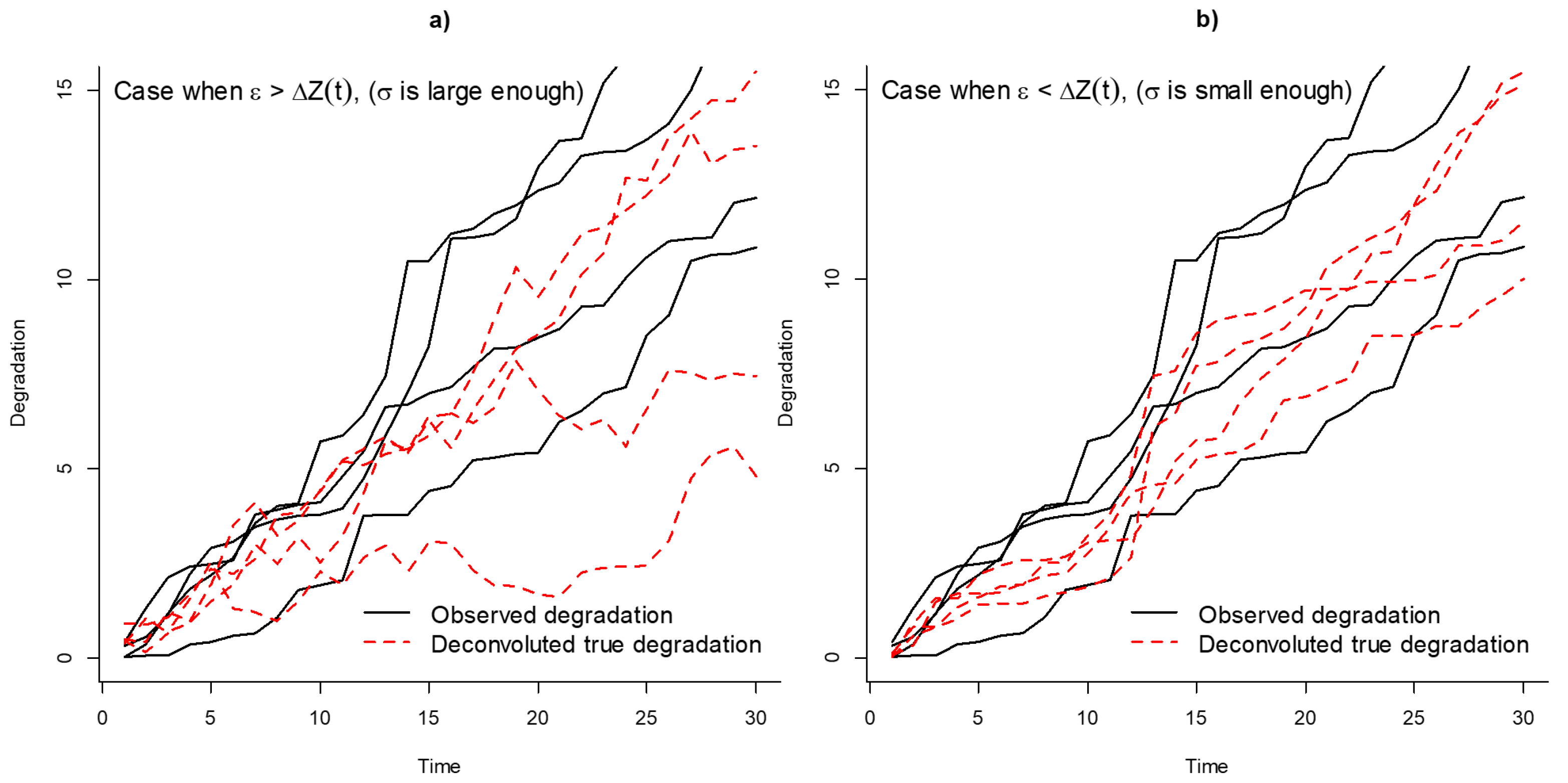
It should be noted that both the gamma and the IG processes are monotone processes, while the Wiener process is known to be non-monotone. If the observed degradation paths are monotone, then it is expected that the true degradation paths remain monotone. Which, can only be true when $\sigma$ is small enough to sustain that $\Delta Z_i\left(t_j\right)>{ϵ}_{ij}$. If $\sigma$ is large enough such that $\Delta Z_i\left(t_j\right)<{ϵ}_{ij}$, then the degradation paths may become non-monotone, which in some case studies may not be reasonable (such as in crack propagation data). Given that in this paper it is considered that the observed degradation paths are governed by a gamma process, it is expected that the true degradation remains governed by a monotone stochastic process. In Figure 1, a comparison of observed degradation paths and deconvoluted true degradation paths is presented when $\Delta Z_i\left(t_j\right)>{ϵ}_{ij}$ and $\Delta Z_i\left(t_j\right)<{ϵ}_{ij}$. The paths with black lines were simulated from a gamma process. From Figure 1a, it can be noted that if $\sigma$ is large enough the true deconvoluted degradation paths become non-monotone. While in Figure 1b, it can be noted that if $\sigma$ is small enough, the deconvoluted paths remain monotone.

The construction of the deconvoluted paths (red dashed lines in Figure 1) is performed considering that the deconvolution operation is performed at every $t_j$ for every degradation measurement $Z_i\left(t_j\right)$. Then, random true measurements of $S_i\left(t_j\right)$ are generated at every $t_j$ to construct the different paths, which represents cumulative sums of the generated random variables. Once the best fitting stochastic process of $W\left[k\right]$ is defined, the true first-passage time distribution can be obtained. The lifetime of the true degradation is defined as $T_s=inf\left\{t_s:S_i\left(t_j\right)\ge \omega \right\}$. The first-passage time distribution will depend on the best fitting stochastic process.

4. The Effect of the Measurement Error over the First-Passage Time Distributions

It is expected that the measurement error affects the behavior of the first-passage time distributions of the observed degradation and the true degradation. If the measurement error is not considered in the modeling, the reliability assessment may be underestimated. For these reasons, it is important to study the effect of the measurement error over the first-passage time distributions, such that a maximum level of error in the measurement system can be determined to obtain a desired reliability assessment. The analysis in this section is focused on determining the differences between the PDF of $T_o$ and $T_s$. Si et al. [4] proposed to compare two first-passage time distributions via the coefficient of variation (CV) and the variation $\left(Var\left(T\right)\right)$ of two distributions. They implemented such approach in a Wiener model with measurement error. The CV can describe the amount of variability in any random variable, thus it is expected that the difference between the CV of $T_o$ and $T_s$ is relatively small if the effect of measurement error is small. The same approach can be considered if the corresponding variations $Var\left(T\right)$ and means $E\left(T\right)$ are compared. In this article, the indices proposed by Si et al. [4] are considered and described in (12) and (13) for the CV and variances, respectively. In addition, an index considering the means is proposed in (14). In fact, any percentile $\left(z_q\right)$ of interest of the first-passage time distributions can be compared as described in (15).

$$I_{CV}\left(T_s,T_o\right)=\frac{\left|CV\left(T_s\right)-CV\left(T_o\right)\right|}{CV\left(T_o\right)}.$$

(12)

$$I_{Var}\left(T_s,T_o\right)=\frac{\left|Var\left(T_s\right)-Var\left(T_o\right)\right|}{Var\left(T_o\right)}.$$

(13)

$$I_E\left(T_s,T_o\right)=\frac{\left|E\left(T_s\right)-E\left(T_o\right)\right|}{E\left(T_o\right)}.$$

(14)

$$I_{z_q}\left(T_s,T_o\right)=\frac{\left|z_q\left(T_s\right)-z_q\left(T_o\right)\right|}{z_q\left(T_o\right)}.$$

(15)

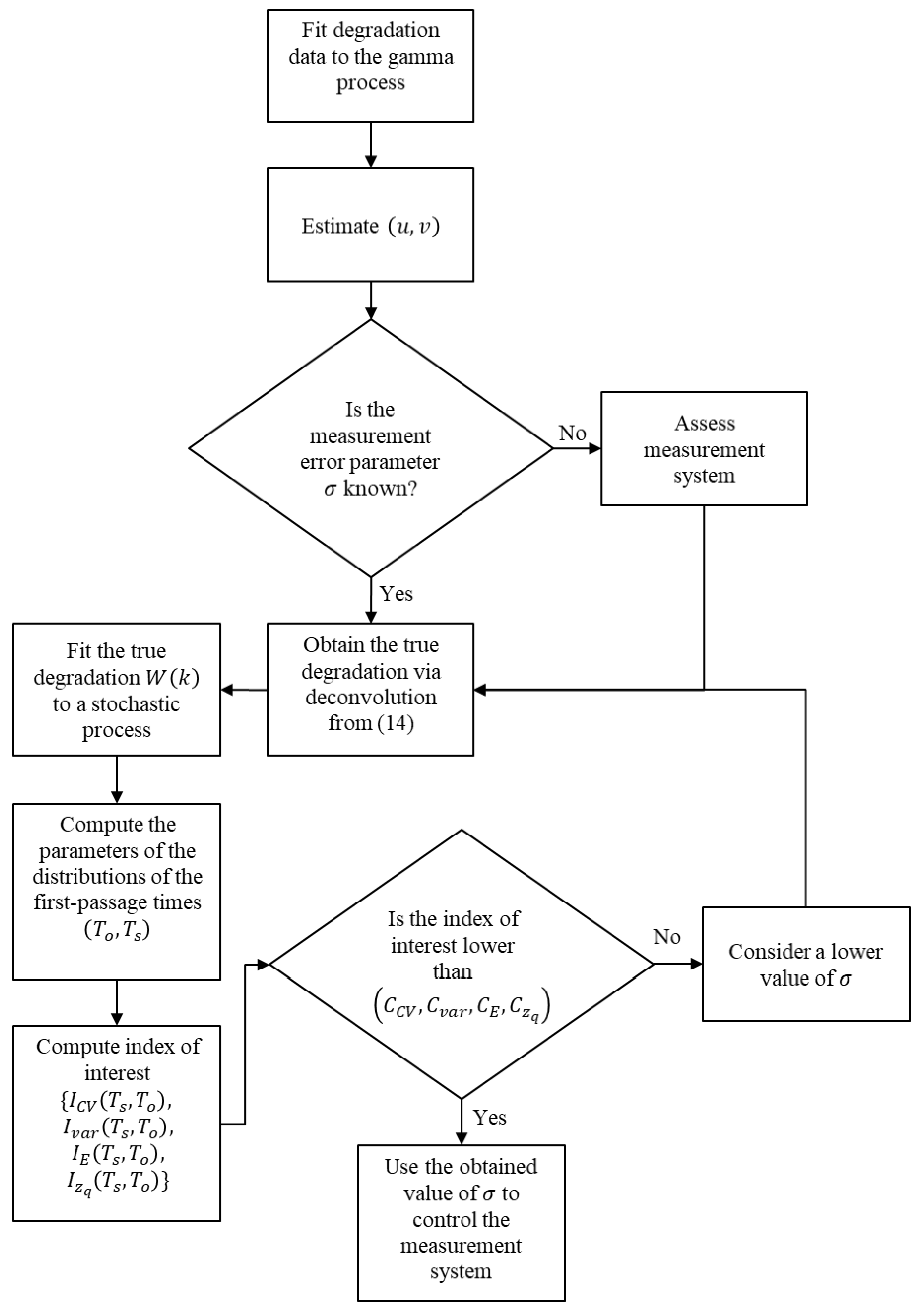
The four indices are considered to describe the differences between the first-passage time distributions. In this way, it is expected that the four indices do not exceed critical values $\left(C_{CV},C_{var},C_E,C_{z_q}\right)$, which means that the estimated lifetime obtained from the distribution $F_{T_o}\left(t\right)$ can approach to the estimation of the distribution $F_{T_s}\left(t\right)$ under certain permissible level of measurement error described in the four critical levels $\left(C_{CV},C_{var},C_E,C_{z_q}\right)$. The flow chart in Figure 2 is followed to optimize $\sigma$ in order to establish a control over the measurement system for a certain accuracy of the reliability assessment of interest.

5. Case Study

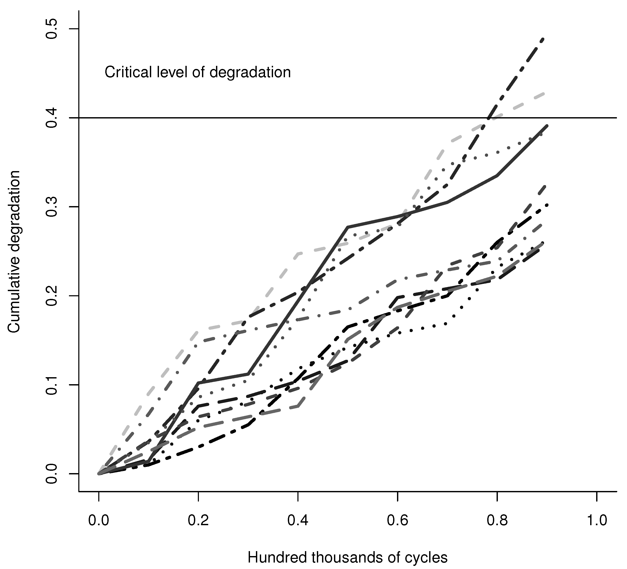
The dataset presented by Rodríguez-Picón et al. [52] is considered for the implementation of the proposed approach. This case study consists in the crack-growth of a terminal in an electronic device. The function of this terminal is to transfer a signal to a receptor, which can be disrupted if the crack in the terminal propagates to a certain critical level, and thus would lead to a failure of the device. A DT was carried out to study the propagation of the crack in 10 terminals. The crack propagation was measured every 0.1 hundred thousand cycles until 0.9 hundred thousand cycles. In this article, it is considered that a failure is said to have occurred when the length of the crack exceeds the critical length of 0.4 mm. The total of sample devices are $N=10$, with $M=9$ observation times as $j=1,2,3,4,5,6,7,8,9$, which are the same for all the $i=1,2,\cdots ,10$ samples with $t_j=(0.1,0.2,0.3,0.4,0.5,0.6,0.7,0.8,0.9)$ hundred thousand cycles. In

Table 1. Degradation dataset of crack-growth case study.

Device	Hundred Thousands of Cycles
	0	0.1	0.2	0.3	0.4	0.5	0.6	0.7	0.8	0.9
1	0	0.01	0.03	0.055	0.107	0.165	0.183	0.2	0.26	0.302
2	0	0.09	0.161	0.172	0.247	0.259	0.281	0.371	0.401	0.429
3	0	0.01	0.06	0.081	0.118	0.142	0.158	0.169	0.232	0.262
4	0	0.016	0.076	0.087	0.104	0.127	0.198	0.208	0.218	0.258
5	0	0.036	0.096	0.176	0.204	0.242	0.281	0.325	0.415	0.495
6	0	0.014	0.102	0.112	0.194	0.277	0.289	0.305	0.335	0.391
7	0	0.037	0.064	0.078	0.096	0.124	0.164	0.234	0.254	0.326
8	0	0.035	0.086	0.105	0.174	0.267	0.277	0.347	0.361	0.384
9	0	0.067	0.148	0.161	0.173	0.184	0.218	0.229	0.239	0.285
10	0	0.025	0.052	0.064	0.076	0.151	0.187	0.205	0.222	0.262

, the degradation measurements are presented, the units are millimeters. In Figure 3, the cumulative degradation paths are presented.

It is assumed that the degradation data in Table 1 are governed by a gamma process as in (4). Thus, $Z_i\left(t_j\right)$ is the observed degradation for $i=1,2,\cdots ,10$, and $t_j=(0.1,0.2,0.3,0.4,0.5,0.6,0.7,0.8,0.9)$. In this case study, it is considered that the measurement error is described by a Gaussian distribution with $\mu =0$ and $\sigma$, as described in (5). Thus, by considering the flow chart in Figure 2, we first estimate the parameters of the gamma process for the degradation dataset in Table 1, then we estimate $\sigma$ by performing an R&R study to the measurement system. Next, we illustrate the effect of the measurement error over the true degradation distribution by using the deconvolution modeling proposed in (9), and to assess the effect over the free-error first-passage time distribution by using the indices presented in ((12)–(15)).

5.1. Estimation of Parameters for the Observed Degradation

The parameters of the observed degradation $\left(u,v\right)$ are estimated via Bayesian approach by considering informative gamma prior distributions for the unknown parameters $\left(u,v\right)$, as $v\sim Ga\left(\zeta ,\eta \right),u\sim Ga\left(\delta ,\tau \right)$. Where, the shape parameters are $\zeta =52.79$ and $\delta =41.45$, and the scale parameters are $\eta =0.4257$ and $\tau =4.13\times {10}^{-4}$, for v and u, respectively. The Markov chain Monte Carlo (MCMC) algorithm is utilized to sample from the joint distribution based on the Gibbs sampler. 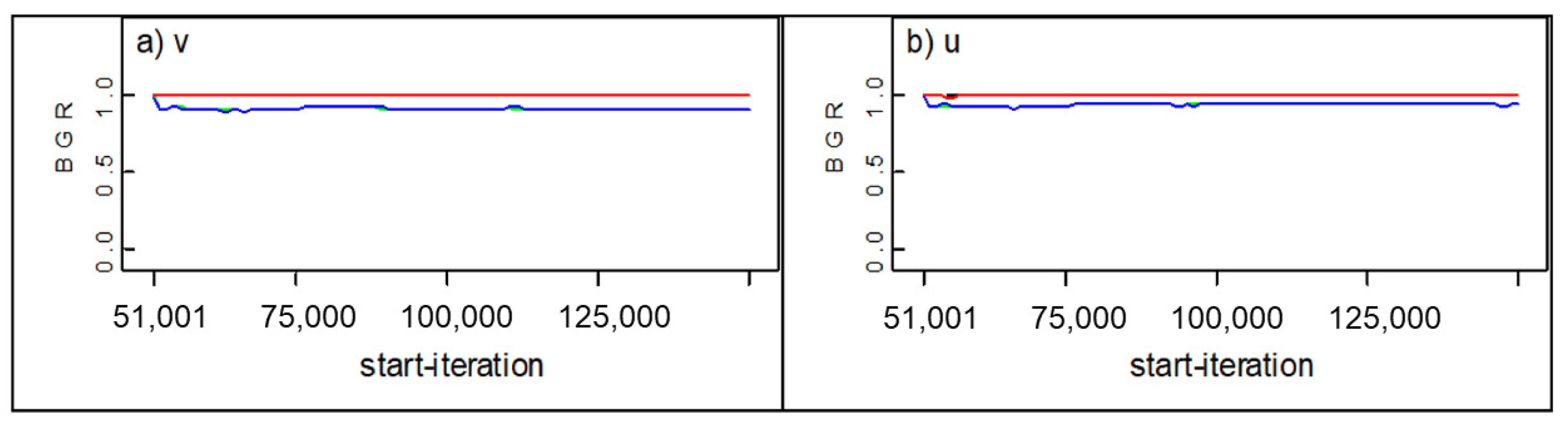For this, a code is developed in the software OpenBUGS [53]. A total of 50,000 iterations were considered for burn-in purposes and 100,000 iterations were considered for estimations purposes. The obtained estimations for the mean, standard deviation, Monte Carlo error, and some percentiles for the parameters $\left(u,v\right)$ are presented in

Table 2. Obtained estimations for the observed degradation.

Parameter	Mean	Sd	MC Error	${\mathit{p}}_{0.025}$	${\mathit{p}}_{0.5}$	${\mathit{p}}_{0.975}$
v	22.55	3.094	0.01476	16.93	22.39	29.02
u	0.01664	0.002687	$1.76\times {10}^{-5}$	0.0126	0.01658	0.02309

. Two sets of initial values are considered in order to assess the convergence of the parameters with the Brooks–Gelman–Rubin (BGR) statistic, the obtained graphs from OpenBUGS are presented in Figure 4. It is considered that convergence is achieved if all the lines in Figure 4 transpose in 1 [54]. It can be noted that convergence is achieved in both parameters.

The first-passage time distribution of the observed degradation is obtained from (3). By considering the mean estimates from Table 2, and $z_0=0$, the parameters can be obtained from ${\alpha }_o^{*}=\sqrt{u/\left(\omega -z_0\right)}$ and ${\beta }_o^{*}=\left(\omega -z_0\right)/uv$ as ${\widehat{\alpha }}_o^{*}=0.2039$ and ${\widehat{\beta }}_o^{*}=1.066$. With these estimates, it is easy to compute the mean and variance as $E\left(T_o\right)=1.088$ and $Var\left(T_o\right)=0.223$, thus $CV\left(T_o\right)=0.434$.

5.2. Characterization of the Measurement Error and Its Effect

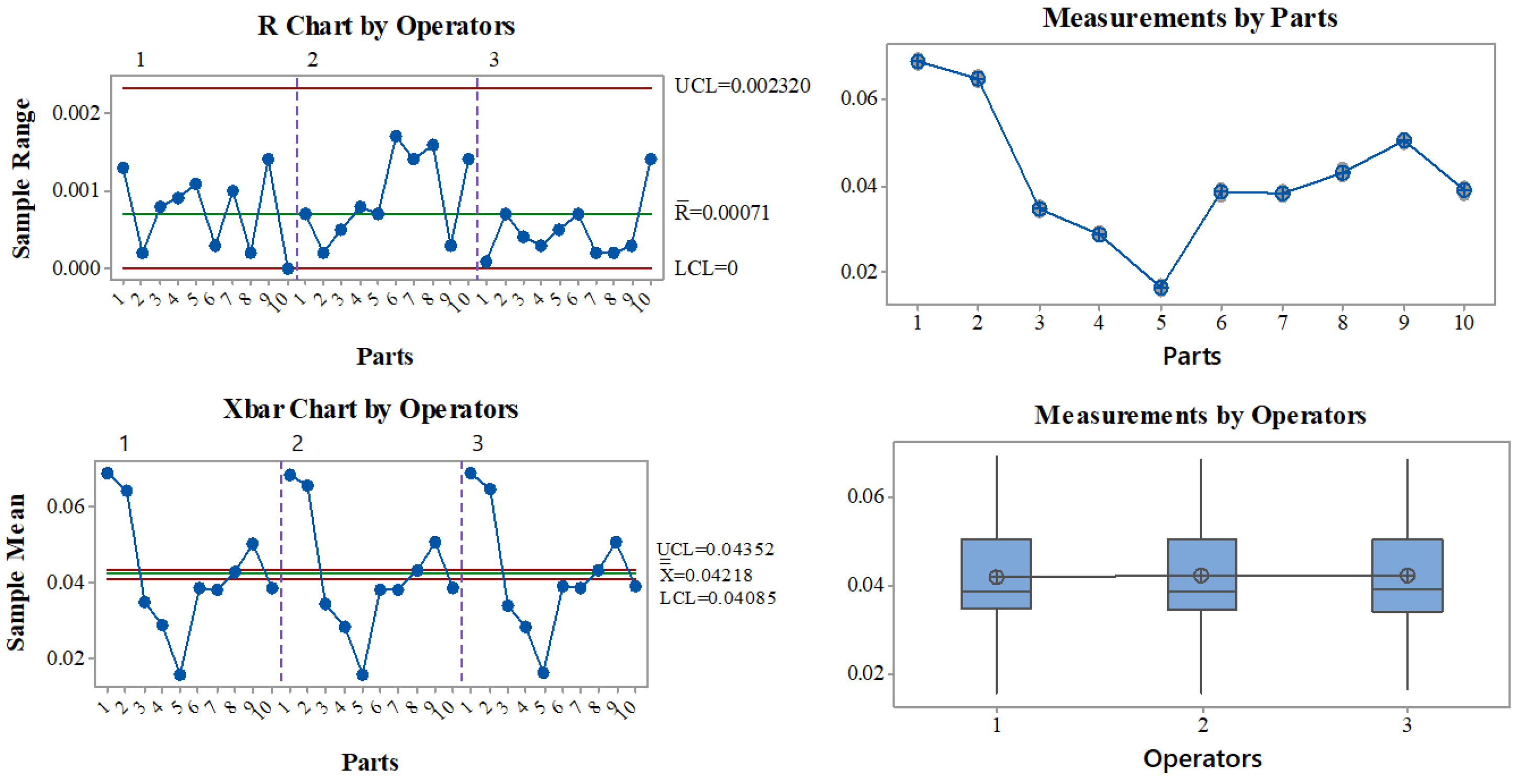
The degradation increments in Table 1 were measured using a vision system with special software applications to measure crack propagations. As $\sigma$ is unknown, we performed an R&R study to assess the performance of the measurement system and to determine how much of the observed variation is due to the measurement system variation, i.e., $\sigma$. The study was performed under the next characteristics: a total of three people were selected to perform the study, 10 devices were selected, and three replicates were performed, making a total of 60 readings. The results of the gage R&R study are presented in

Table 3. Gage R&R variation contribution.

Source	StdDev (SD)	Study Variation (6*SD)	% Study Variation
Total gage R&R	0.0006058	0.0036347	3.83
Repeatability	0.0006058	0.0036347	3.83
Reproducibility	0.0000000	0.0000000	0.00
Operators	0.0000000	0.0000000	0.00
Part to Part	0.0157952	0.0947713	99.93
Total Variation	0.0158068	0.0948409	100

and Figure 5. It can be noted from Table 3 that the total variation contribution of the repeatability and reproducibility are 3.83% and 0.00%, respectively, which makes the total gage R&R contribution at 3.83%. The general rule says that if the total gage R&R contribution is less than 10%, the measurement system is acceptable, which is the case of this study. From Figure 5, it can be noted that indeed the measurement system performs well, and that most of the variation comes from the part-to-part variation.

From Table 3, the standard deviation of the gage R&R study is ${\sigma }_{R\&R}=0.0006058$, which is the total variation due to the measurement system. Thus, we consider ${\sigma }_{R\&R}$ as an estimation of $\sigma$, such that $\widehat{\sigma }={\sigma }_{R\&R}=0.0006058$, and use this value to perform the deconvolution approach presented in Section 3.

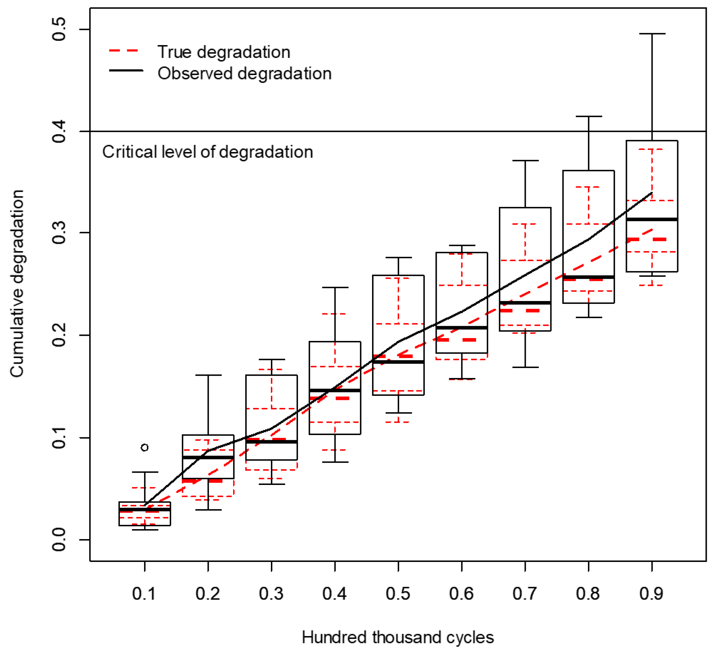
Considering the estimated parameters in Table 2 for the gamma process, we estimated $q_g$ for every $t_j$. Then, we implemented the deconvolution approach considering $\widehat{\sigma }=0.0006058$ and $p=1000$. In Figure 6, a comparison of the observed degradation paths and the obtained true deconvoluted degradation paths is provided by presenting the box plots and mean for every $t_j$. It can be noted from Figure 6 that the variation in every $t_j$ was reduced in the true deconvoluted paths. In addition, the mean degradation in every $t_j$ is smaller in the true deconvoluted paths than the observed paths as in the work of Rodriguez-Picon et al. [30]. It is obvious, that the reduction in the variation at every $t_j$ will cause variations in the mean degradation, i.e., degradation rate, as can be noted in both degradation paths. Indeed, these conditions will have an impact on the first-passage time distributions.

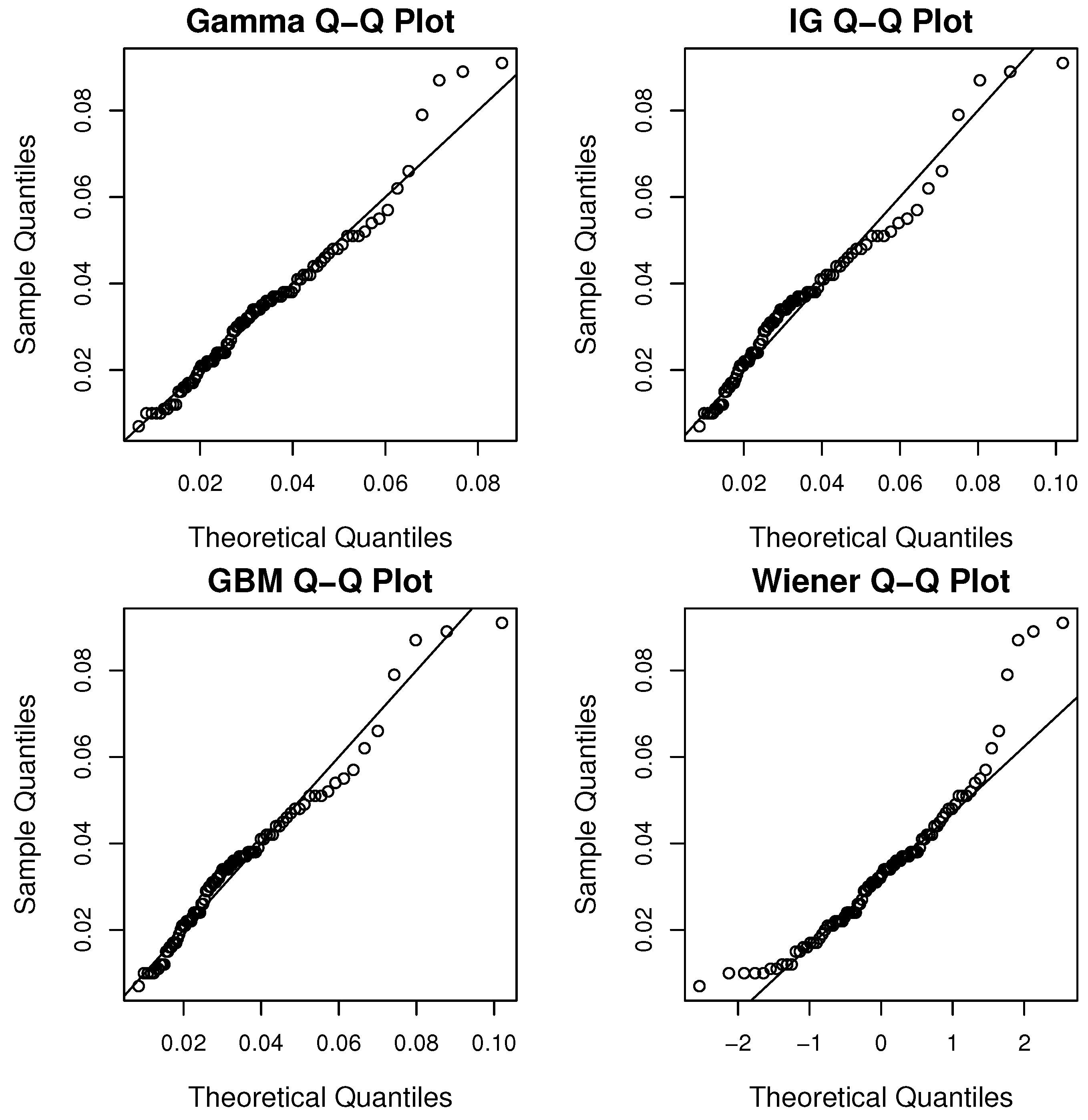
As the true degradation function does not have an analytical closed form, we consider to fit the obtained true degradation to the gamma, IG, GBM and Wiener stochastic processes. Stochastic models are considered to describe temporal uncertainty, such as the observed degradation is modeled with the gamma process. Although, a simple approximation can be defined when obtaining cumulative sums of the true deconvoluted variables. To perform a reliability assessment of such approximation, the Kaplan–Meier method can be considered to define the reliability function. In order to assess the goodness of fit of the four stochastic processes we consider a graphical method such as the Q-Q plots. In Figure 7, the Q-Q plots for the different stochastic processes are presented for the true degradation.

It can be noted from Figure 7 that the gamma process seems to have a better fit. In addition to the Q-Q plots, we also performed the Cramér–von Mises goodness of fit test for all the models. The obtained Cramér–von Mises statistics were, for gamma 0.056918, for IG 0.20057, for GBM 0.1748 and for Wiener 0.18345. By considering the critical value for the Cramér–von Mises statistic for a significance level of 0.1 of 0.173, it can be noted that the gamma process is the only one not rejected. Thus, we consider the gamma process to govern the true deconvoluted degradation.

5.3. Comparison of the First-Passage Time Distributions

It is considered that the vector $W\left[k\right]$ is described by a gamma process as $Ga(v^{*}\Delta t_j,u^{*})$ with shape parameter $\left(v^{*}\Delta t_j\right)$, and scale parameter $\left(u^{*}\right)$. The true first-passage time distribution can be obtained by considering the Birnbaum–Saunders distribution with parameters ${\alpha }_s^{*}=\sqrt{u^{*}/\left(\omega -z_0\right)}$ and ${\beta }_s^{*}=\left(\omega -z_0\right)/v^{*}{u}^{*}$, with $z_0=0$, and $\omega =0.4$. Thus, the CDF is described as

$$F_{T_s}\left(t\right)=\Phi \left[\frac{1}{{\alpha }_s^{*}}\left(\sqrt{\frac{t}{{\beta }_s^{*}}}-\sqrt{\frac{{\beta }_s^{*}}{t}}\right)\right],$$

(16)

with mean obtained as $E\left(T_s\right)={\beta }_s^{*}\left(1+{\alpha }_s^{*2}/2\right)$, and the variance as $Var\left(T_s\right)={\alpha }_s^{*}{\beta }_s^{*}$${\left(1+5{\alpha }_s^{*2}/4\right)}^{1/2}$.

The estimated gamma parameters of the true degradation were obtained as ${\widehat{v}}^{*}=37.9237$ and ${\widehat{u}}^{*}=0.0088$. Considering these estimates, the parameters of the first-passage time distributions for the true degradation can be easily obtained considering the Birnbaum–Saunders distribution. The computed parameters were obtained as ${\widehat{\alpha }}_s^{*}=0.1483$ and ${\widehat{\beta }}_s^{*}=1.1985$. In

Table 4. Comparison of the mean, variance and CV for the first-passage times of the observed and true degradation.

	Mean	Variance	CV
Observed	1.088	0.223	0.434
True	1.211	0.18	0.1487

, a comparison of the the mean, variance, and CV for the observed and true first-passage time distributions is presented.

From Table 4, the effect of the measurement over the first-passage time distribution is reflected. For instance, the mean passage-time from the true degradation is greater that the obtained from the observed degradation. In addition, the variance is smaller for the true degradation compared to the observed degradation. This finding can be confirmed by the degradation paths described in Figure 6, where the mean degradation and the variation among degradation paths are smaller compared to the observed degradation.

The distributions $f_{T_o}\left(t\right)$ and $f_{T_s}\left(t\right)$ are compared by computing the indices described in ((12)–(15)) as denoted in the flow chart in Figure 2. The 5th percentile is considered for (15). The quantile function of the Birnbaum–Saunders distribution is described as [55],

$$t\left(q\right)=\beta {\left(\frac{\alpha z_q}{2}+\sqrt{\frac{{\alpha }^2{z}_q^2}{4}+1}\right)}^2,$$

where $z_q$ is the $q\times 100$th quantile of the standard normal distribution. Considering that $z_5=-1.6448$ and the estimates ${\widehat{\alpha }}_o^{*}$, ${\widehat{\beta }}_o^{*}$ and ${\widehat{\alpha }}_s^{*}$, ${\widehat{\beta }}_s^{*}$, the 5th percentile for the first-passage time distributions for the observed and true degradation were obtained as $t_o\left(5\right)=0.7633$ and $t_s\left(5\right)=0.9396$, respectively. All four indices described in Section 4, $I_{CV}\left(T_s,T_o\right)$, $I_{Var}\left(T_s,T_o\right)$, $I_E\left(T_s,T_o\right)$, $I_{z_5}\left(T_s,T_o\right)$ were computed and are presented in

Table 5. Computed indices from the observed and true first-passage time distributions.

	${\mathit{I}}_{\mathbf{CV}}\left({\mathit{T}}_{\mathit{s}},{\mathit{T}}_{\mathit{o}}\right)$	${\mathit{I}}_{\mathbf{Var}}\left({\mathit{T}}_{\mathit{s}},{\mathit{T}}_{\mathit{o}}\right)$	${\mathit{I}}_{\mathit{E}}\left({\mathit{T}}_{\mathit{s}},{\mathit{T}}_{\mathit{o}}\right)$	${\mathit{I}}_{{\mathit{z}}_5}\left({\mathit{T}}_{\mathit{s}},{\mathit{T}}_{\mathit{o}}\right)$
Index	0.6574	0.1919	0.1136	0.2309

.

The critical values $\left(C_{CV},C_{var},C_E,C_{z_5}\right)$ may be defined depending of the allowance for the measurement error of the measurement system. In this paper, four indices are considered, however, one index can be used depending of the reliability estimation of interest. As can be noted from ((12)–(15)), the indices are ratios that account for the relative increase in each reliability estimation, i.e., CV, variance, mean, percentiles. Indeed, the greater the value of the respective indices the more difference between reliability estimations, which means more variability of the measurement error, i.e., $\sigma$. Critical values should be defined based on historical behavior, but a first approach can be considered as follows: consider that the measurement system has been evaluated and an estimation of $\sigma$ is obtained, then the true and observed first-passage time distributions can be characterized. Consider that $\sigma$ is a component of variance with good performance, i.e., less than 10% of the total variation of the process [56]. If the mean is the estimation of interest, then from (14) it can be considered that $C_E=I_E$, this equivalence of the critical value will relate the good performance of the measurement system to the estimation of the mean failure time, so the control scheme can be initiated. Now consider a specific example, if the critical values are considered as $C_{CV}=0.66,C_{Var}=0.2,C_E=0.12$, and $C_{\left(z_5\right)}=0.24$, it is observed from Table 5 that the standard deviation for the measurement error $\sigma =0.0006058$ is good enough for the performance of the measurement system. With this parameter of the measurement error, it is expected that the estimated lifetime from the data contaminated with measurement error should be accurate enough. It should be noted that $\sigma$ may be optimized by following the sequence determined in the flow chart in Figure 2. However, previous knowledge of the case study must be available such that optimal values of the critical values $\left(C_{CV},C_{var},C_E,C_{z_1}\right)$ are defined. For instance, the mean time to failure (MTTF) of the observed degradation and the true degradation with $\sigma =0.0006058$ are $E\left(T_o\right)=1.088$, and $E\left(T_s\right)=1.211$, respectively. Which means a difference of 0.123 hundred thousands of cycles. If the maximum allowance for the difference between MTTF is expected to be, for example, 0.05 hundred thousands of cycles and the critical value $C_E=0.043$, it can be noted that $I_E\left(T_s,T_o\right)$ is higher $C_E$ which means that the measurement system should be improved such that the measurement process is executed more accurately and the variation caused by the measurement system is reduced. The same approach may be considered for any other index different than $C_E$, depending on the estimation of interest. For example, if it is expected that the differences between the 5th percentiles of the failure times for the observed degradation and the true degradation be 0.09 hundred thousands of cycles and $C_{z_5}=0.105$, again it can be noted that $I_{z_5}>C_{z_5}$, which denotes a high variance of the measurement error.

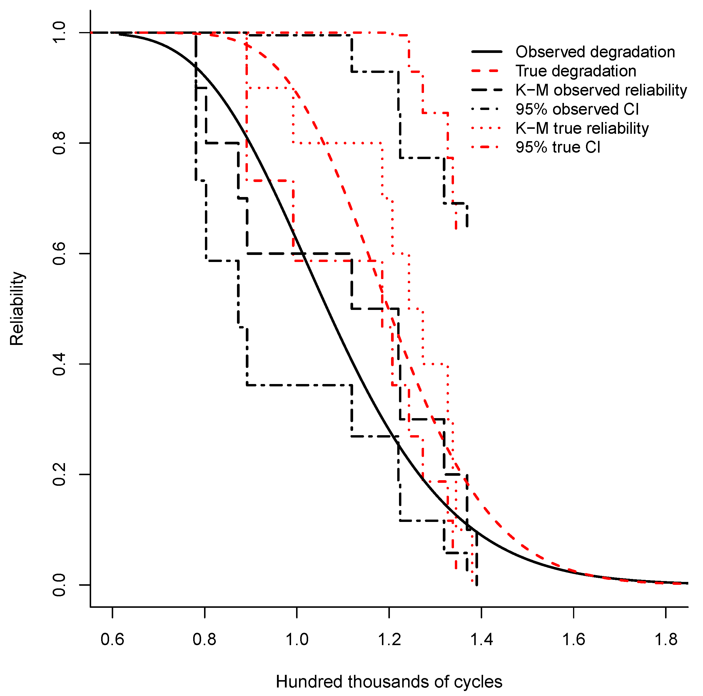
The reliability functions with and without measurement error were obtained based on the corresponding first-passage time distributions. The respective differences can be noted in Figure 8. Along with the respective reliability functions, we also present the Kaplan–Meier reliability for the observed and true degradation, along with their respective 95% confidence intervals. At different $t_j$, the Kaplan–Meier confidence interval of the true reliability does not include the observed reliability, which denotes the difference. A difference of the reliability functions presented by Rodriguez-Picon et al. [30], apart from the considered stochastic processes for the observed degradation, relies on that, in this paper, a stochastic process is fitted to the true degradation which defines the dashed red reliability function. Furthermore, the reliability estimation from Kaplan–Meier results in a different behavior as the true degradation comes from a gamma-Gaussian deconvolution.

6. Extension for Non-Gaussian Measurement Errors

Other PDFs can be considered to describe the measurement error in the proposed approach. As the deconvolution operation is performed based on CFs, the proposed method can be extended to more PDFs by replacing the corresponding CF in the denominator of (8). Then, the approximation of the true degradation can be obtained by implementing the fast Fourier transform in (10) and (11). In this section, we illustrate this extension by considering that the measurement error follows a logistic distribution $f_L\left({\epsilon }_{ij}|{\mu }_L,s\right)$. The CF is presented as follows,

$${\phi }_{\epsilon }\left(\zeta \right)=exp\left\{i\zeta {\mu }_L\right\}\frac{\pi s\zeta }{sinh\left(\pi s\zeta \right)},$$

(17)

Then, the CF of the true measurement is defined as,

$${\phi }_S\left(\zeta \right)=\frac{{\left(1-ui\zeta \right)}^{-v}}{exp\left\{i\zeta {\mu }_L\right\}\frac{\pi s\zeta }{sinh\left(\pi s\zeta \right)}},$$

(18)

The CF in (18) is considered in (11) to obtain the true measurements. The parameters of the observed degradation are presented in Table 2 as $v=22.55$ and $u=0.01664$. From the R&R study, it is known that the total variation due to the measurement system is $\widehat{\sigma }={\sigma }_{R\&R}=0.0006058$. For this scenario, it is considered that ${\mu }_L=0$, and as the standard deviation of the logistic distribution is defined as $SD=\sqrt{(s^2{\pi }^2/3)}$, then by considering $SD=0.0006058$ it follows that $s=0.0033$. The deconvolution approach is implemented considering these parameters with $p=1000$. The vector $W\left[k\right]$ was then fitted to the gamma, Wiener, inverse Gaussian and GBM processes. It was found that the gamma process is the best fitting model. 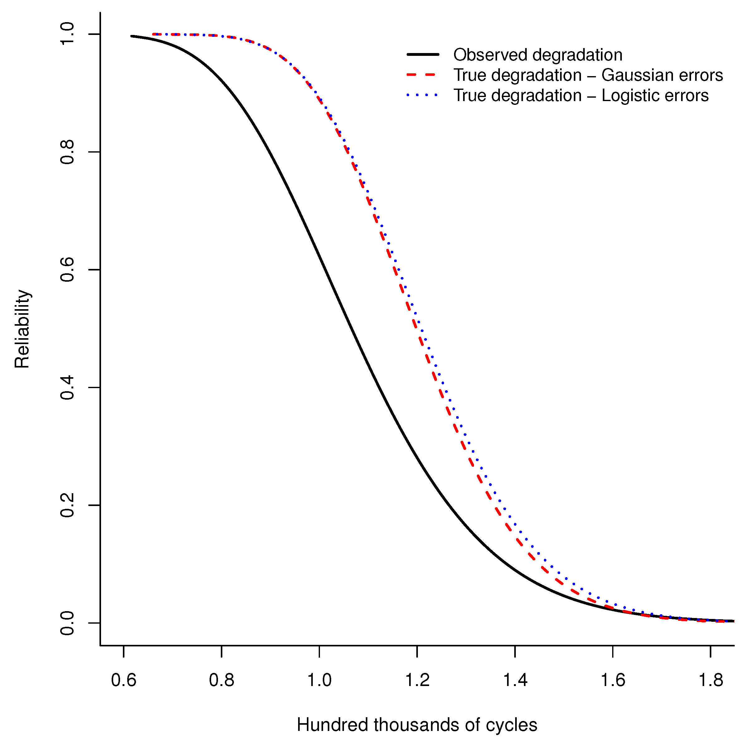The reliability function based on the estimated parameters of the first-passage time distributions with logistic errors is compared with the Gaussian errors in Figure 9. It can be noted that the behavior of the reliability functions is quite similar. With the logistic errors, the reliability is estimated to be greater when $t>1.1$ hundred thousand cycles, approximately. It is known that the logistic distribution has higher kurtosis than the Gaussian distribution, which may account for the small differences in the reliability function. Both reliability functions, estimated considering measurement error, determine that the true degradation has greater reliability than the observed degradation.

7. Concluding Remarks and Discussion

The reliability assessment of products is a critical activity for different processes and systems, thus it is important to consider that the analyzed data are free of any contamination that can cause inaccurate conclusions. Furthermore, as the measuring process is an integral part of reliability testing, it is also important to establish some control schemes over the measuring system’s performance. Such that, a certain performance of the system leads to a predetermined performance of the product’s reliability assessment. In the case of degradation modeling, the measuring error causes variation in the first-passage time distribution. Based on this, it may be expected that the reliability assessment under contaminated data may be underestimated. In this article, it is considered that a gamma process governs the observed degradation with measurement error, and it is assumed that the error can be described by a Gaussian distribution with mean zero and standard deviation $\sigma$. Thus, the true degradation is obtained by deconvoluting the observed degradation and the measurement error. In order to control the measurement error in terms of the reliability assessment, the first-passage time distributions of the observed and the true degradation are compared in terms of some proposed indices. A general scheme was proposed to establish the differences between distributions in order to obtain the desired accuracy of the assessment. From the case study, it was observed that depending on the reliability estimation of interest; it is possible to establish a maximum level of the standard deviation of the measurement error. This enables to control the measuring system. It is essential to define critical levels of the indices for the first-passage time distributions, such that a maximum level of error can be established. These critical values can be defined by considering the maximum difference between the reliability estimation of interest between the true and contaminated first-passage distributions. Following the proposed scheme, the permissible error can be determined as described in the case study. Furthermore, a scenario to deal with non-Gaussian measurement errors is presented to extend the deconvolution approach applicability.

There are several opportunities for further research in the proposed scheme of this article. Although the gamma process has been widely used in degradation modeling, other stochastic processes can be used to describe the observed degradation, such as the inverse-Gaussian process, geometric Brownian motion and the Wiener process. The deconvolution modeling proposed in this paper can be extended by considering any of these processes. Although, the implementation for some process may result more complex, as the CFs of the inverse Gaussian and geometric Brownian motion do not have closed expressions, which impose interesting challenges for the implementation of the deconvolution approach. Furthermore, other sources of uncertainty can be included in the degradation modeling. It has been found that the consideration of random effects accounts for the accuracy of the reliability estimations. Indeed, these sources imply certain mathematical complexity which should be added to the computational complexity of the deconvolution approach. For this, different deconvolution algorithms proposed in the literature may be considered to obtain approximations of true variables obtained from measurement error contaminated processes. The CV, variation, mean and percentiles are considered as indices to measure the differences between first-passage time distributions. Nevertheless, some other metrics can be studied with the same purpose. In addition, we consider some well-known stochastic processes to model the true degradation as an approximation, given that the function of the true degradation does not have a closed analytical expression. However, further investigation may be directed in the future to study the deconvoluted function of gamma and Gaussian distributions.