Abstract
Monitoring rock damage subjected to cracks is an important stage in underground spaces such as radioactive waste disposal repository, civil tunnel, and mining industries. Acoustic emission (AE) technique is one of the methods for monitoring rock damage and has been used by many researchers. To increase the accuracy of the evaluation and prediction of rock damage, it is required to consider various AE parameters, but this work is a difficult problem due to the complexity of the relationship between several AE parameters and rock damage. The purpose of this study is to propose a machine learning (ML)-based prediction model of the quantitative rock damage taking into account of combined features between several AE parameters. To achieve the goal, 10 granite samples from KAERI (Korea Atomic Energy Research Institute) in Daejeon were prepared, and a uniaxial compression test was conducted. To construct a model, random forest (RF) was employed and compared with support vector regression (SVR). The result showed that the generalization performance of RF is higher than that of SVRRBF. The R2, RMSE, and MAPE of the RF for testing data are 0.989, 0.032, and 0.014, respectively, which are acceptable results for application in laboratory scale. As a complementary work, parameter analysis was conducted by means of the Shapley additive explanations (SHAP) for model interpretability. It was confirmed that the cumulative absolute energy and initiation frequency were selected as the main parameter in both high and low-level degrees of the damage. This study suggests the possibility of extension to in-situ application, as subsequent research. Additionally, it provides information that the RF algorithm is a suitable technique and which parameters should be considered for predicting the degree of damage. In future work, we will extend the research to the engineering scale and consider the attenuation characteristics of rocks for practical application.
1. Introduction
Monitoring rock damage induced by cracks is an important stage in underground spaces such as radioactive waste disposal repository, civil tunnel, and mining industries. The occurrence of rock damage begins from microcracks. As these cracks propagate and bond each other, an excavation damaged zone (EDZ) is formed near the facility [1]. The EDZ affects the degradation of the rock properties which leads to a decrease in the facility’s stability. Most of the rock damage occurs immediately after excavation due to stress disturbance and redistribution, but in the deep geological environment, the progressive damage of the rock is generated due to high in-situ stress.
The occurrence of cracks is accompanied by an increase of the specimen’s volume. Thus, the volume change is related to the degree of damage in the rock sample [2]. Based on this principle, Martin and Chandler [3] and Martin et al. [4] determined a crack damage criterion using crack volumetric strain. They divided a damage evolution into four stages: crack closure (), crack initiation (), crack coalescence (), and crack damage () (Figure 1). Crack closure stress is defined as the point at which the axial stiffness curve changes from nonlinear to linear or where the crack volumetric strain converges to zero. The crack initiation stress is defined by the onset of stable crack growth and is indicated as the point at which the crack volumetric strain deviates from zero. Therefore, the range between crack closure and crack initiation is considered as the region showing elastic behavior. Meanwhile, the crack coalescence is referred to as the point where large irregularities in the volumetric stiffness occur. The crack damage stress is characterized by unstable growth of crack and associated with the reversed region in the curve of the total volumetric strain [1,5].
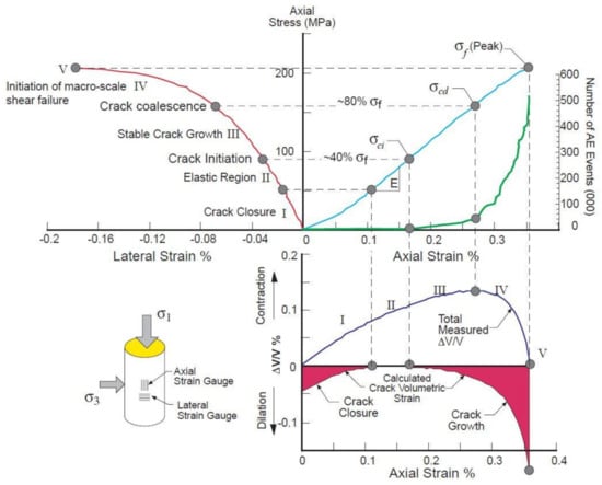
Figure 1.
Typical stressstrain plot for crack growth of rocks (Martin et al. [4]). A crack damage threshold can be divided into four stages using volumetric stiffness and crack volumetric strain: crack closure (), crack initiation (), crack coalescence (), and crack damage ().
In recent years, the use of acoustic emission (AE) in underground spaces has been increased. AE technique is a kind of nondestructive method to monitor crack growth in a brittle material. When a material is subjected to a progressive load and cracks develop, it would lead to a sudden release of strain energy of the material, which generates an elastic stress wave from cracks of the materials. Many researchers used AE method to associate crack damage of brittle rocks [1,6,7]. Ranjith et al. [8] used an AE event to correlate rock damage growth. They observed the change of the curve trend of cumulative AE count and then characterized crack evolution into four stages. Some researchers tried to correlate crack evolution characteristics with AE count from the uniaxial compression test [1,9]. Wu et al. [10] evaluated the quantitative damage stress using cumulative AE count. The results showed that the AE cumulative count curve is divided into three stages according to the axial stress level: the slowly increasing stage, the steady stage, and the sharply increasing stage. Hatton et al. [11] and Cox et al. [12] evaluated the degree of rock damage using the b-value originating from seismology, which is calculated from a relation of AE amplitude and AE frequency. Later, Shiotani and Ohtsu [13] improved the b-value taken into account for a signal attenuation according to AE sensors location. Carpinteri et al. [14] concluded that the b-value reflects the initiation and propagation of cracks in pre-peak stage in the investigation of the AE from different sized rock. Kim [15] performed a uniaxial compression test for granite specimens and confirmed that the rock damage estimated from the cumulative AE energy is similar to the damage for the crack volumetric strain. Subsequently, he extended the scope of application to the in-situ rock in consideration of crack size and wave attenuation [16]. Zhao et al. [17] studied the relation between crack development and AE hit for Beishan granite. The result showed that the number of AE hit increased as the stress increased and increased sharply as the stress is close to rock failure. There are some works to evaluate the failure pattern of rock damage based on multi-AE parameters [18,19]. They classified the rock failure into shear and tensile mode by using AE frequency and RA value which is a multi-AE parameter obtained from dividing the AE rise time by the AE amplitude. Yang et al. [20] introduced damage-related indicators such as AE activity and AE fault total area which are relevant to AE magnitude and AE event for predicting a rock failure precursor.
The aforementioned research gives insights into evaluating the rock damage using different AE parameters, such as AE event or hit, amplitude, frequency, energy, count, and rise time. To increase the accuracy of the evaluation and prediction of rock damage, it is necessary to consider various AE parameters, but this work is a tough problem due to the complexity of the relationship between several AE parameters and rock damage. In recent years, machine learning (ML) techniques have been utilized to analyze the complex relationship between inputs and targets in the field of rock engineering with AE technique, such as crack recognition [21], crack localization for rocks [22], ultrasonic wave-based damage detection [23], and damage identification using ultrafast wave scattering simulation [24]. However, there is no ML-based predictive model for quantitative damage of rocks. Among the various ML algorithm, ensemble-based random forest (RF) gives different advantages for modeling: (1) it is a kind of ensemble model that combines a variety of single decision trees to improve the predictive power and overcome outliers, (2) it has been validated to have a better predictive power compared with a single ML-based model in the literature [25,26].
The purpose of this study is to propose an ML-based prediction model of the quantitative rock damage taking into account of combined features between several AE parameters. In the main study, 10 granite samples from KAERI (Korea Atomic Energy Research Institute) in Daejeon are prepared, and a uniaxial compression test under the condition of progressive loading in laboratory scale is executed to obtain the dataset, including the AE parameters and the degree of rock damage based on crack volumetric strain [27]. To consider combined features between rock damage and various AE parameters, ML-based random forest (RF) is employed and compared with support vector regression (SVR). As a complementary work, parameter analysis is conducted by means of the recently published Shapley additive explanations (SHAP) [28] for model interpretability. The rest of this paper is organized as follow: Section 2 presents the process of experimental test and illustrates ML-based technique; Section 3 covers the result and discussion, and Section 4 describes a conclusion.
2. Experimental Test and Machine Learning Technique
2.1. Sample Preparation and Uniaxial Compression Test
To execute the uniaxial compression test, we obtained the granite (RG-2) from KAERI (Korea Atomic Energy Research Institute) in Daejeon, South Korea. (Figure 2). KURT was constructed for the purpose of simulating the radioactive waste disposal environment [29]. With consideration of the practical purpose for achieving the required depth, the tunnel has a downward slope of 10% and a size of 6 × 6 m. The geological formation of KURT generally comprises Mesozoic two-mica granite, and detailed topographic and geological information and host rock conditions of this site can be found in the literature [29]. Ten granite samples were collected from 56.2 to 60.8 m depth and made by satisfying the NX size suggested by ISRM (2007) [30] as shown in Figure 3. The flatness of the initial and end surfaces was adjusted to less than 0.02 mm.
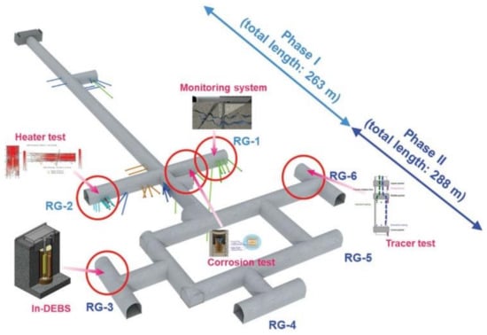
Figure 2.
Korea Underground Research Tunnel (KURT) located in Daejeon, South Korea. This facility was constructed for the purpose of simulating the radioactive waste disposal repository.
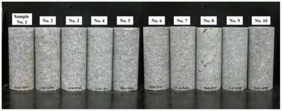
Figure 3.
Ten granite specimens to be used in the compression test. These were obtained from the RG-2 section in KURT which comprises Mesozoic two-mica granite.
A uniaxial compression test was carried out and the deformation and failure behavior of samples were observed. The average ratio of length to diameter for specimens is 2.4, which is somewhat lower than 2.4 suggested by ISRM (2007) [30]. Biaxial strain gauges (AP-11-TS50N-120-EC, CAS) with a data logger (UCAM 20PC, KYOWA) were attached to the rock surface for monitoring the rock deformation according to the vertical stress level in increments of 0.2 MPa/s (Figure 4). The tests were conducted by increasing the loading rate of 0.19–0.21 MPa/s on the specimens using the stress-controlled mode to simulate the progressive damage of rocks. Figure 5 shows a representative stress–strain curve for sample No. 2. A description of this curve will be given in Section 2.2. Testing times from the stress initiation to the rock failure were recorded as 9–17 min. The descriptive statistics for the rock properties are summarized in Table 1.
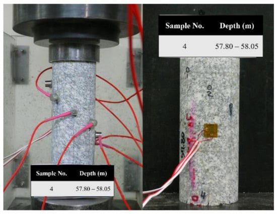
Figure 4.
Bi-axial strain gauge and eight acoustic emission sensors attached to the specimen surface. The strain gauge was installed to the center of the vertical axis and AE sensors were attached in a spiral direction for a wide range of crack detection.
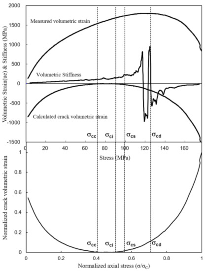
Figure 5.
Volumetric strain and stiffness curves (sample No. 2) with respect to the stress level in the increment of 0.2 MPa/s. The degree of damage for granite was calculated by normalizing the crack volumetric strain after crack initiation stress level ().

Table 1.
Descriptive statistics of 10 granite specimens collected from KURT.
Simultaneously, eight AE sensors (AE603SW-GA), which have a sensitivity of 115 dB, a valid frequency of 30–300 kHz, and a resonance frequency of 60 kHz, were used to acquire AE signals. For ensuring reliable data, the sensors were attached to the rock specimen using an epoxy bond (Araldite Rapid corporation: relative density of −1.17 at 25 Celsius, specific acoustic impedance of 12.8 × 10⁶ kg/m2 · s), eliminating the air and minimizing the measurement error in the acoustic impedance [31]. The AE voltage was amplified to 60 dB for detection efficiency using a preamplifier. As a data acquisition system, a RECTUSON 10-channel analyzer was used, where the peak definition time, hit definition time, and hit locking time were specified as 50, 100, and 500 s to extract the signal concerning rock crack. The threshold of a lower limit for AE signal detection was set to 65 dB. Additionally, only signals obtained from the sensor attached to the middle of the specimen were considered under the detected condition by more than 6 out of 8 AE sensors. The AE voltage was amplified to 60 dB for detection efficiency using a preamplifier. To remove the noise of AE signals, filtering with wavelet transform was used. The specifications of equipment used for the uniaxial compression test are summarized in Table 2.
Table 2.
Equipment specification for uniaxial compression and acoustic emission test.
2.2. Degree of Rock Damage and AE Parameters
From the result of the compression test, the volumetric strain, stiffness, and in-elastic volumetric strain were calculated to evaluate the degree of damage for rocks according to the vertical stress level (loading rate: 0.2 MPa/s) (Figure 5). The in-elastic volumetric strain can be calculated by the Equations (1) and (2) based on the stress–strain relationship;
where, is a volumetric strain, is an elastic volumetric strain, and indicates the in-elastic volumetric strain. and mean the axial and lateral strain. , and indicate the elastic modulus, Poisson’s ratio, and axial stress, respectively. Martin [32] defined this in-elastic volumetric strain as the crack volumetric strain that is attributed to axial cracking and proposed using the crack volumetric strain to characterize a crack initiation. Based on this principle, in this study, the crack volumetric strain was associated with rock damage to quantify the degree of damage. The crack volumetric strain can be calculated by subtracting an in-elastic volumetric strain by their maximum value. By normalizing the crack volumetric strain, the degree of damage is finally calculated.
In this study, the degree of damage only higher than the crack initiation stress () was considered as valid values to collect the reliable dataset. Here, the crack initiation stress refers to the stress point at which the crack volumetric strain becomes zero [3]. If the stress level is lower than the crack initiation stress, the crack closure is dominant in this range, not crack initiation [1].
From the AE data acquisition system, we also collected the AE dataset for 10 granite specimens. As AE input parameters were chosen, an amplitude, hit, count, rise time, absolute energy, and initiation frequency were selected through the literature review in Section 1. A visual explanation of these AE parameters is depicted in Figure 6.
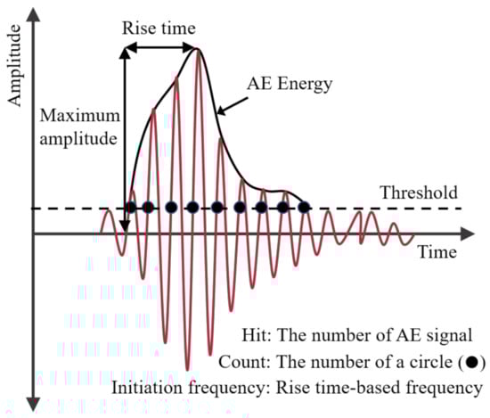
Figure 6.
Example of six acoustic emission (AE) parameters in an AE signal. In this study, these AE parameters were transformed as cumulative values and used as inputs for predicting the degree of rock damage.
2.3. Machine Learning Technique
2.3.1. Single Model: Support Vector Regression
Support vector regression (SVR), proposed by Vapnik et al. [33], is a kind of supervised learning technique This method has a generalization ability even with restricted number of dataset since it is based on the principle of structural risk minimum rather than empirical risk minimization [34]. Here, generalization ability means the state that is not overfitting for specific and biased data.
SVR is not sensitive to margin error () and learns to include as many datasets as possible in a limited -tube (Figure 7). Even if the training set is newly added, the errors are considered as zero within the allowed . However, if the training sets are outside the ε-tube, a non-zero value of the slack variable () occurs, which indicates the degree of margin violation. Based on the above principle, SVR can be composed of the optimization problem (Equation (3)) that has a global optimum point;
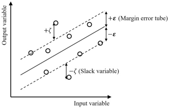
Figure 7.
Concept of support vector regression. It learns to include as many datasets as possible in a limited -tube and a constraint of the slack variable. Even if the training set is newly added, the errors are regarded as zero within the allowed ε. However, if the training set is outside the ε-tube, a non-zero value of the slack variable (ζ) occurs, which indicates the degree of margin violation.
Equation (3) must be subject to the following conditions;
where, and are an input vector and actual output. is a weight vector of input vector. is a regularization parameter indicating a penalty for the sample error exceeding the margin. A larger value means a smaller slack variable is allowed, whereas a smaller value means a larger slack variable is allowed. is a function that maps the input space of the training set into a high-dimensional feature space. To solve the Equation (3), Lagrangian dual formulation, which includes a dot product between two functions, should be calculated. Fortunately, the dot product between functions can be easily calculated as a kernel function () as shown in Equation (7);
plays the role of expanding the input space of the training sets into a high-dimensional space, which makes it possible to express a nonlinearity problem. Since the related theory is out of the scope of this study, it is recommended to refer to the literature [33]. There are several types of established by researchers, and the functions used in this study are summarized in Table 3.
Table 3.
Representative kernel functions of SVR used in this study.
2.3.2. Ensemble Model: Random Forest
Random forest (RF), suggested by Breiman [35], is one of the ensemble techniques composed of a bunch of decision trees (DT) [36]. The DT is a decision support algorithm that uses a tree-like model of decisions and their possible output. The DT algorithm is conducted by partitioning a data space into subspace. During the building of a DT, three components are created, namely internal node, terminal node, and branch of DT. The internal node is linked with decision functions to determine which next node to face. The terminal node is the node that is no longer to be separated in a DT. This node is the space to classify samples that fall into the node. Branch of DT plays a role of connecting internal and external nodes in a DT.
RF is more powerful algorithm and has been validated to be more robust in many more data sciences than a DT [25,37]. The principle behind the RF is to create a variety of overfitted DTs in different directions and is to average the results of each DT. It is an effective way to reduce the overfitting problem. DTs can be implemented by randomly sampling the dataset for each DT (bagging) and by selecting an input parameter randomly (Figure 8). RF is the convenient method in that it does not need to consider the data scales and works properly without the delicate hyper-parameter tuning. A detailed explanation and theory of RF can be found in [35].
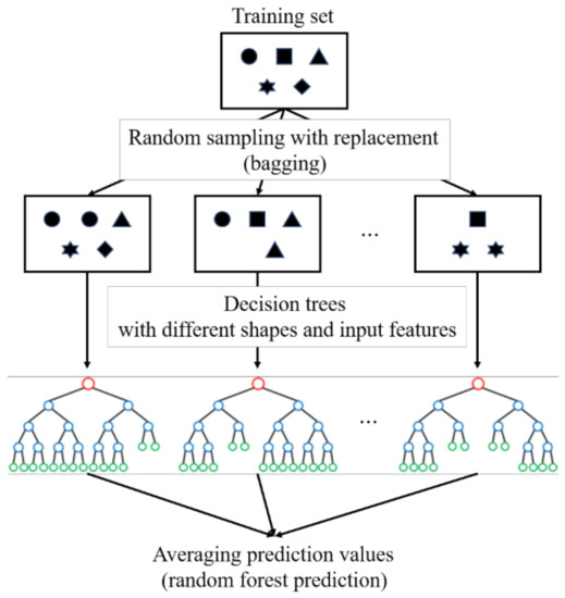
Figure 8.
Principle of a random forest (RF). Bagging is the process of data sampling from a training set, randomly. Sampled datasets are used to make different kinds of decision trees (DTs). In the prediction phase, all the values predicted from various DTs are averaged and it is called the prediction value of RF.
3. Result and Discussion
3.1. Data Preparation
The mechanical data points from the compression test were recorded in units of 0.1 MPa, while AE data points are only recorded when the valid cracks are detected in the rock sample. For matching the two different types of dataset, a smooth spline approximation for 10 granite specimens was used. The AE parameters used in this study were AE amplitude, hit, count, rise time, absolute energy, and initiation frequency. These six parameters were converted to cumulative values and used as inputs for predicting the degree of rock damage. Figure 9 shows the scatter plots for the relationship between inputs and output. Although 10 granite specimens were extracted from the same borehole in RG-2 section, the curves for each input showed different trends. This phenomenon seems to be due to the difference of properties such as rock strength, stiffness, and Poisson’s ratio (Table 1) and shows that predicting the degree of rock damage using only one or two AE parameters is a difficult problem.
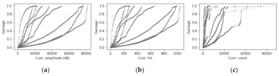
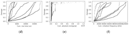
Figure 9.
The changes of the damage for cumulative AE parameters such as (a) amplitude, (b) hit, (c) count, (d) rise time, (e) absolute energy, and (f) initiation frequency. Although 10 granite specimens were extracted from the same borehole in RG-2 section, the curves for each input showed different trends. This phenomenon seems to be due to the difference of properties such as rock strength, stiffness, and Poisson’s ratio and indicates that predicting the degree of rock damage using only one or two AE parameters is a difficult problem.
To prepare a dataset for ML-based models, the inputs values were normalized in the range from 0 to 1 for eliminating a scale effect. The entire dataset (5301 data points) was divided into training (80%) and testing (20%) set, randomly. Here, the training set was used for model training and hyper-parameter tuning, while the testing set was used for model evaluation [38].
3.2. Model Optimization and Generalization Performance
To select the best model, the hyper-parameter set should be optimized. This process is the essential step because the performance of a model varies significantly depending on the hyper-parameter set. The procedure of optimizing a model is divided into five stages: (1) a hyper-parameter tuning space is specified; (2) an arbitrary hyper-parameter set within a given range is chosen using random-search method. Here, random-search is the method sampling hyper-parameter set randomly in the range of specified tuning space; (3) a model is built for the training set with a given hyper-parameter set and is evaluated through cross-validation. Here, the cross-validation is the one of validation methods used for selecting the optimum hyper-parameter set in the given space. The principle of cross-validation is to divide a training set into k-folds, and then one fold is used as the validation data for the model which is fitted by the rest of folds. This process is repeated k times and all the outputs are evaluated through evaluation metric; (4) after repeating the stage 3 several times, only the hyper-parameter set with the best value of evaluation metric is chosen; (5) based on the hyper-parameter set selected from the stage 4, the stages 1–4 are repeated until the hyper-parameter set converges to the optimum set. From the process, final hyper-parameter space and optimum set selected are summarized in Table 4. As for an evaluation metric, the RMSE was selected and the equation can be expressed as Equation (8);
where is the actual output and is the corresponding predicted output. The RMSE history for the final cycle of stage 5 according to the models such as random forest (RF), linear and nonlinear support vector regression (SVRLinear, SVRRBF) are shown in Figure 10. Here, the vertical axis indicates the result of the sorted root mean squared error (RMSE) in descending order. The results show that the RMSE for SVRLinear and SVRRBF were 0.182 and 0.104, respectively. In other words, the performance of SVRRBF showed about 1.8 times higher than that of the SVRLinear. This result implies that the relationship between the AE parameters and the degree of damage is a complex and nonlinear problem. As for comparison between two different nonlinear models, the RF (RMSE = 0.048) showed 2.2 times higher optimizing performance than the SVRRBF (RMSE = 0.104).
Table 4.
Hyper-parameter tuning spaces and optimized values for each ML method.
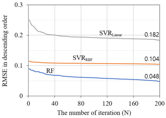
Figure 10.
Cross-validated RMSE in descending order versus the number of iterations. The results show that the performance of SVRRBF is about 1.8 times higher than that of the SVRLinear. This result implies that the relationship between the AE parameters and the degree of damage is a complex and nonlinear problem. As for comparison between two different nonlinear models, the RF (RMSE = 0.048) showed 2.2 times higher optimizing performance than the SVRRBF (RMSE = 0.104).
To verify a generalization performance, the optimized nonlinear models were examined for a testing set that was not used to construct the models (Figure 11). As evaluation indices for the models, R-squared (R2), RMSE, and mean absolute percentage error (MAPE) were selected in this study and the formulation of R2 and MAPE can be expressed as Equations (9) and (10), respectively;
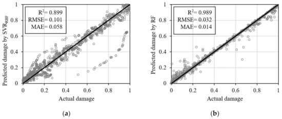
Figure 11.
Actual damage versus the damage predicted by (a) SVRRBF and (b) RF for the testing set. The solid line indicates the relationship . Data points for a good prediction would lie close to the solid line. In Figure 11a, some data points far from the solid line seem to have increased the prediction error. On the other hand, the data points in Figure 11b were overall close to a solid line, which indicates that RF is higher generalization performance compared with SVRRBF.
In Figure 11, the solid line indicates the relationship . Data points for a good prediction would lie close to the solid line. The result showed that R2, RMSE, MAPE for the SVRRBF were 0.899, 0.101, and 0.058, whereas as for the RF, the values were 0.989, 0.032, and 0.014, respectively. In Figure 11a, some data points far from the solid line seem to have increased the prediction error. On the other hand, the data points in Figure 11b were overall close to a solid line, which indicate that RF is higher generalization performance compared with SVRRBF. Based on the results, we selected the RF model as the best fitting model and their information is summarized in Table 4.
3.3. Parameter Analysis
To capture an insight for the RF model, not only predictive performance but also model interpretability should be accompanied simultaneously. The Shapley additive explanations (SHAP) proposed by Lundberg and Lee [28] is the integrated framework for interpreting the model’s prediction, which can express each parameter importance for a specific prediction to magnitudes and directions. The SHAP value is based on Shapley values originated from coalitional game theory and a local interpretable model agnostic explanation (LIME) that gives insights for local interpretability. The LIME value has a limitation of being unfair in terms of collaborative game theory. To complement this shortcoming, the SHAP value improved this unfairness of LIME by employing the Shapley value. A detailed explanation and theory of SHAP can be found in [28].
In this study, SHAP analysis for the RF model was performed (Figure 12). In this graph, an individual point represents the SHAP value of each dataset. The higher the SHAP value, the higher the positive contribution to the damage value. On the other hand, the lower the SHAP value, the higher the negative contribution to the damage value. The degree of ‘high’ and ‘low’ values for the parameter can be distinguished by colors ‘red’ and ‘blue’, respectively. As shown in Figure 12, the degree of contribution to the damage value for the cumulative absolute energy strongly increased when the cumulative absolute energy increased. In general, the cumulative energy is related to the energy released by the crack growth of the rock [39] and is known to be directly proportional to the actual energy of the rock [27]. The result suggests that AE absolute energy is still the main parameter that has a major influence on the degree of damage even under the condition considering various AE parameters. The cumulative initiation frequency also contributed to the damage value positively when this value also increased. The distribution of frequency is known to be concerned with the stress level including rock type and the degree of fracturing [40]. Based on the result, an AE frequency seems to be definitely associated with the degree of damage, but it is unsuitable to use alone due to the low importance relatively. In addition, since the value varies with the type of AE sensor and the adhesion condition to rock [41], AE frequency should be considered with several AE parameters.
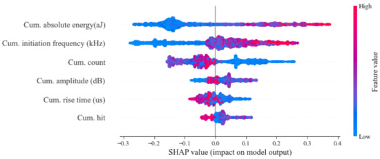
Figure 12.
Distribution of SHAP values for cumulative AE parameters. An individual point represents the SHAP value of each dataset. The higher the SHAP value, the higher the positive contribution to the damage value. On the other hand, the lower the SHAP value, the higher the negative contribution to the damage value. The degree of ‘high’ and ‘low’ values for the parameter can be distinguished by colors ‘red’ and ‘blue’, respectively.
For a better understanding of these results, we plotted the force plots for specific data points corresponding to a high and low damage level, respectively (Figure 13). In the case of a data point belonging to the high level of damage (0.99), it was confirmed that the cumulative absolute energy and initiation frequency strongly give a positive contribution to the damage value (Figure 13a). In the opposite case at which the damage value is 0.02, the above two parameters strongly offered a negative contribution to the damage value (Figure 13b). Figure 14 shows the absolute average of the SHAP values for each parameter. The result showed that the average value of the cumulative absolute energy is 0.152, which is the highest value among the several AE parameters. This result is in good agreement with several studies [15,42,43]. Obviously, other parameters also contribute to the prediction of rock damage. These results provide rationality for considering various AE parameters for predicting the degree of rock damage.
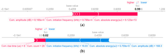
Figure 13.
Force plots of specific data points in (a) high damage and (b) low damage level. In the case of a data point belonging to the high level of damage (0.99), it was confirmed that the cumulative absolute energy and initiation frequency strongly give a positive contribution to the damage value (Figure 13a). In the opposite case at which the damage value is 0.02, the above two parameters strongly offered a negative contribution to the damage value (Figure 14b).
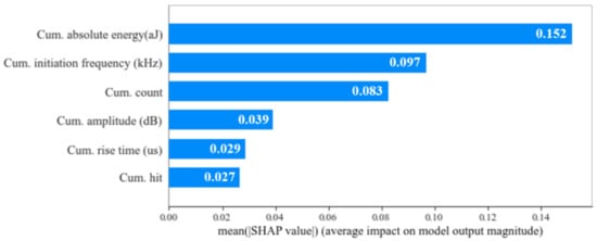
Figure 14.
Averaged absolute values of SHAP. The result showed that the cumulative absolute energy is the highest value among the several AE parameters. Obviously, other parameters also contribute to the prediction of rock damage. These results provide rationality for considering various AE parameters for predicting the degree of rock damage.
4. Conclusions
Monitoring rock damage induced by cracks is an important stage in geotechnical engineering. AE technique is a useful method for monitoring rock damage and has been used by many researchers. To increase the accuracy of the evaluation and prediction of rock damage, it is necessary to consider various AE parameters, but this work is a tough problem due to the complexity of the relationship between several AE parameters and rock damage. In this study, we proposed a random forest-based prediction model of the quantitative rock damage taking into account combined features between several AE parameters. To fulfill this purpose, 10 granite samples from KAERI in Daejeon were prepared, and a uniaxial compression test under the condition of progressive loading in laboratory scale was conducted to obtain the dataset, including the AE parameters and the degree of rock damage based on crack volumetric strain. To consider combined features between rock damage and various AE parameters, an RF algorithm was employed and compared with SVR. As an additional work, parameter analysis was conducted by means of the SHAP for model interpretability. The conclusions derived from the results can be summarized as follows;
- It was confirmed that the relationship between cumulative AE parameters and the degree of damage shows a strong nonlinear tendency by comparing SVRRBF with SVRLinear;
- The R2, RMSE, and MAPE of the RF for the testing set was 0.989, 0.032, and 0.014 respectively, which are higher generalization performance than that of SVRRBF and are acceptable results for application in the laboratory scale;
- In both high and low levels degree of the damage, the cumulative absolute energy and initiation frequency were selected as the main parameters affecting the prediction of the damage. However, care should be taken that the initiation frequency should be considered with several AE parameters since this value is sensitive to the type of AE sensor and the adhesion condition to a rock surface;
- Other AE parameters such as AE count, amplitude, rise time, and hit also contributed to the prediction of rock damage. These results provide rationality for considering various AE parameters for predicting the degree of rock damage.
Although the results of this simulation model cannot be used directly to make predictions in situ due to the scale effect, discontinuity, and attenuation characteristics for in-situ rocks, this study suggests the possibility of extension to in-situ application in underground spaces, as subsequent research. Additionally, it provides information that the RF algorithm is a suitable technique and which parameters should be considered for predicting the degree of damage. In future work, we will extend the research to the engineering scale and consider the attenuation characteristics of rocks for practical application.
Author Contributions
Conceptualization, H.-L.L.; methodology, H.-L.L.; writing—original draft, H.-L.L., J.-S.K., C.-H.H., and D.-K.C.; writing—review and editing, H.-L.L., J.-S.K., C.-H.H., and D.-K.C.; All authors have read and agreed to the published version of the manuscript.
Funding
This research was also supported by the Nuclear Research and Development Program of the National Research Foundation of Korea (NRF-2021M2C9A1018633) funded by the Minister of Science and ICT.
Institutional Review Board Statement
Not applicable.
Informed Consent Statement
Not applicable.
Data Availability Statement
Not applicable.
Conflicts of Interest
The authors declare no conflict of interest.
References
- Eberhardt, E.; Stead, D.; Stimpson, B.; Read, R.S. Identifying crack initiation and propagation thresholds in brittle rock. Can. Geotech. J. 1998, 35, 222–233. [Google Scholar] [CrossRef]
- Lin, Q. Strength Degradation and Damage Micromechanism of Granite under Long-Term Loading. Bachelor’s Thesis, University of Hong Kong, Hong Kong, China, 2006. [Google Scholar]
- Martin, C.; Chandler, N. The progressive fracture of Lac du Bonnet granite. Int. J. Rock Mech. Min. Sci. Géoméch. Abstr. 1994, 31, 643–659. [Google Scholar] [CrossRef]
- Martin, C.D.; Christiansson, R.; Söderhäll, J. Rock Stability Considerations for Siting and Constructing a KBS-3 Repository. Based on Experiences from Aespoe HRL, AECL’s URL, Tunnelling and Mining; Swedish Nuclear Fuel and Waste Management Co.: Stockholm, Sweden, 2001. [Google Scholar]
- Diederichs, M.; Kaiser, P.; Eberhardt, E. Damage initiation and propagation in hard rock during tunnelling and the influence of near-face stress rotation. Int. J. Rock Mech. Min. Sci. 2004, 41, 785–812. [Google Scholar] [CrossRef]
- Cai, M.; Morioka, H.; Kaiser, P.; Tasaka, Y.; Kurose, H.; Minami, M.; Maejima, T. Back-analysis of rock mass strength parameters using AE monitoring data. Int. J. Rock Mech. Min. Sci. 2007, 44, 538–549. [Google Scholar] [CrossRef]
- Rudajev, V.; Vilhelm, J.; Lokajíček, T. Laboratory studies of acoustic emission prior to uniaxial compressive rock failure. Int. J. Rock Mech. Min. Sci. 2000, 37, 699–704. [Google Scholar] [CrossRef]
- Ranjith, P.; Jasinge, D.; Song, J.; Choi, S. A study of the effect of displacement rate and moisture content on the mechanical properties of concrete: Use of acoustic emission. Mech. Mater. 2008, 40, 453–469. [Google Scholar] [CrossRef]
- Zhou, H.; Meng, F.Z.; Lu, J.J.; Zhang, C.Q.; Yang, F.J. Discussion on methods for calculating crack initiation strength and crack damage strength for hard rock. Rock Soil Mech. 2014, 35, 913–918. [Google Scholar]
- Wu, C.; Gong, F.; Luo, Y. A new quantitative method to identify the crack damage stress of rock using AE detection parameters. Bull. Int. Assoc. Eng. Geol. 2021, 80, 519–531. [Google Scholar] [CrossRef]
- Hatton, C.; Main, I.; Meredith, P. A comparison of seismic and structural measurements of scaling exponents during tensile subcritical crack growth. J. Struct. Geol. 1993, 15, 1485–1495. [Google Scholar] [CrossRef]
- Cox, S.; Meredith, P. Microcrack formation and material softening in rock measured by monitoring acoustic emissions. Int. J. Rock Mech. Min. Sci. Géoméch. Abstr. 1993, 30, 11–24. [Google Scholar] [CrossRef]
- Shiotani, T.; Ohtsu, M. Prediction of slope failure based on AE activity. In Acoustic Emission: Standards and Technology Update; ASTM International: West Conshohocken, PA, USA, 1999. [Google Scholar]
- Carpinteri, A.; Lacidogna, G.; Accornero, F.; Mpalaskas, A.; Matikas, T.; Aggelis, D. Influence of damage in the acoustic emission parameters. Cem. Concr. Compos. 2013, 44, 9–16. [Google Scholar] [CrossRef]
- Kim, J. Quantitative Damage Assessment of In-Situ Rock Mass Using Acoustic Emission Technique. Ph.D. Thesis, KAIST, Daejeon, Korea, 2013. [Google Scholar]
- Kim, J.-S.; Kim, G.-Y.; Baik, M.-H.; Finsterle, S.; Cho, G.-C. A New Approach for Quantitative Damage Assessment of In-Situ Rock Mass by Acoustic Emission. Geomech. Eng. 2019, 18, 11–20. [Google Scholar]
- Zhao, X.; Cai, M.; Wang, J.; Ma, L. Damage stress and acoustic emission characteristics of the Beishan granite. Int. J. Rock Mech. Min. Sci. 2013, 64, 258–269. [Google Scholar] [CrossRef]
- Rodríguez, P.; Celestino, T.B. Application of acoustic emission monitoring and signal analysis to the qualitative and quantitative characterization of the fracturing process in rocks. Eng. Fract. Mech. 2019, 210, 54–69. [Google Scholar] [CrossRef]
- Zhang, J.Z.; Zhou, X.P.; Zhou, L.S.; Berto, F. Progressive failure of brittle rocks with non-isometric flaws: Insights from acousto-optic-mechanical (AOM) data. Fatigue Fract. Eng. Mater. Struct. 2019, 42, 1787–1802. [Google Scholar] [CrossRef]
- Yang, J.; Mu, Z.-L.; Yang, S.-Q. Experimental study of acoustic emission multi-parameter information characterizing rock crack development. Eng. Fract. Mech. 2020, 232, 107045. [Google Scholar] [CrossRef]
- Wang, C.; Hou, X.; Liu, Y. Three-Dimensional Crack Recognition by Unsupervised Machine Learning. Rock Mech. Rock Eng. 2021, 54, 893–903. [Google Scholar] [CrossRef]
- Ince, N.; Kao, C.-S.; Kaveh, M.; Tewfik, A.; Labuz, J. A Machine Learning Approach for Locating Acoustic Emission. EURASIP J. Adv. Signal Process. 2010, 2010, 895486. [Google Scholar] [CrossRef]
- Rautela, M.; Gopalakrishnan, S. Ultrasonic guided wave based structural damage detection and localization using model assisted convolutional and recurrent neural networks. Expert Syst. Appl. 2021, 167, 114189. [Google Scholar] [CrossRef]
- Yan, W.-J.; Chronopoulos, D.; Papadimitriou, C.; Cantero-Chinchilla, S.; Zhu, G.-S. Bayesian inference for damage identification based on analytical probabilistic model of scattering coefficient estimators and ultrafast wave scattering simulation scheme. J. Sound Vib. 2020, 468, 115083. [Google Scholar] [CrossRef]
- Qi, C.; Tang, X. Slope stability prediction using integrated metaheuristic and machine learning approaches: A comparative study. Comput. Ind. Eng. 2018, 118, 112–122. [Google Scholar] [CrossRef]
- Qi, C.; Fourie, A.; Chen, Q.; Tang, X.; Zhang, Q.; Gao, R. Data-driven modelling of the flocculation process on mineral processing tailings treatment. J. Clean. Prod. 2018, 196, 505–516. [Google Scholar] [CrossRef]
- Kim, J.-S.; Lee, K.-S.; Cho, W.-J.; Choi, H.-J.; Cho, G.-C. A Comparative Evaluation of Stress–Strain and Acoustic Emission Methods for Quantitative Damage Assessments of Brittle Rock. Rock Mech. Rock Eng. 2015, 48, 495–508. [Google Scholar] [CrossRef]
- Lundberg, S.; Lee, S.-I. A unified approach to interpreting model predictions. arXiv 2017, arXiv:1705.07874. [Google Scholar]
- Kim, G.Y.; Kim, K.; Lee, J.-Y.; Cho, W.-J.; Kim, J.-S. Current Status of the KURT and Long-term In-situ Experiments. J. Korean Soc. Miner. Energy Resour. Eng. 2017, 54, 344–357. [Google Scholar] [CrossRef]
- Hatheway, A.W. The Complete ISRM Suggested Methods for Rock Characterization, Testing and Monitoring; 1974–2006. Environ. Eng. Geosci. 2009, 15, 47–48. [Google Scholar] [CrossRef]
- Watanabe, T.; Sassa, K. Velocity and amplitude of P-waves transmitted through fractured zones composed of multiple thin low-velocity layers. Int. J. Rock Mech. Min. Sci. Géoméch. Abstr. 1995, 32, 313–324. [Google Scholar] [CrossRef]
- Martin, C.D. The Strength of Massive Lac du Bonnet Granite around Underground Openings; University of Manitoba: Winnipeg, MB, Canada, 1993. [Google Scholar]
- Vapnik, V.; Golowich, S.E.; Smola, A.J. Support vector method for function approximation, regression estimation and signal processing. Adv. Neural Inf. Process. Syst. 1997, 9, 281–287. [Google Scholar]
- Burges, C.J. A Tutorial on Support Vector Machines for Pattern Recognition. Data Min. Knowl. Discov. 1998, 2, 121–167. [Google Scholar] [CrossRef]
- Breiman, L. Statistical Modeling: The Two Cultures (with comments and a rejoinder by the author). Stat. Sci. 2001, 16, 199–231. [Google Scholar] [CrossRef]
- Song, Y.-Y.; Ying, L. Decision tree methods: Applications for classification and prediction. Shanghai Arch. Psychiatry 2015, 27, 130. [Google Scholar]
- Kuhn, M.; Johnson, K. Applied Predictive Modeling; Springer: Berlin/Heidelberg, Germany, 2013; Volume 26. [Google Scholar]
- Zorlu, K.; Gokceoglu, C.; Ocakoglu, F.; Nefeslioglu, H.; Acikalin, S. Prediction of uniaxial compressive strength of sandstones using petrography-based models. Eng. Geol. 2008, 96, 141–158. [Google Scholar] [CrossRef]
- Landis, E.N.; Baillon, L. Experiments to Relate Acoustic Emission Energy to Fracture Energy of Concrete. J. Eng. Mech. 2002, 128, 698–702. [Google Scholar] [CrossRef]
- Liu, X.; Wu, L.; Zhang, Y.; Liang, Z.; Yao, X.; Liang, P. Frequency properties of acoustic emissions from the dry and saturated rock. Environ. Earth Sci. 2019, 78, 67. [Google Scholar] [CrossRef]
- Ishida, T.; Labuz, J.F.; Manthei, G.; Meredith, P.G.; Nasseri, M.H.B.; Shin, K.; Yokoyama, T.; Zang, A. ISRM Suggested Method for Laboratory Acoustic Emission Monitoring. Rock Mech. Rock Eng. 2017, 50, 665–674. [Google Scholar] [CrossRef]
- Grosse, C.U.; Ohtsu, M. Acoustic Emission Testing; Springer Science & Business Media: Berlin, Germany, 2008. [Google Scholar]
- Khazaei, C.; Hazzard, J.; Chalaturnyk, R. Damage quantification of intact rocks using acoustic emission energies recorded during uniaxial compression test and discrete element modeling. Comput. Geotech. 2015, 67, 94–102. [Google Scholar] [CrossRef]
Publisher’s Note: MDPI stays neutral with regard to jurisdictional claims in published maps and institutional affiliations. |
© 2021 by the authors. Licensee MDPI, Basel, Switzerland. This article is an open access article distributed under the terms and conditions of the Creative Commons Attribution (CC BY) license (https://creativecommons.org/licenses/by/4.0/).