Railway Vehicle Wheel Flat Detection with Multiple Records Using Spectral Kurtosis Analysis

Abstract

The gradual deterioration of train wheels can increase the risk of failure and lead to a higher rate of track deterioration, resulting in less reliable railway systems with higher maintenance costs. Early detection of potential wheel damages allows railway infrastructure managers to control railway operators, leading to lower infrastructure maintenance costs. This study focuses on identifying the type of sensors that can be adopted in a wayside monitoring system for wheel flat detection, as well as their optimal position. The study relies on a 3D numerical simulation of the train-track dynamic response to the presence of wheel flats. The shear and acceleration measurement points were defined in order to examine the sensitivity of the layout schemes not only to the type of sensors (strain gauge and accelerometer) but also to the position where they are installed. By considering the shear and accelerations evaluated in 19 positions of the track as inputs, the wheel flat was identified by the envelope spectrum approach using spectral kurtosis analysis. The influence of the type of sensors and their location on the accuracy of the wheel flat detection system is analyzed. Two types of trains were considered, namely the Alfa Pendular passenger vehicle and a freight wagon.

1. Introduction

The presence of a geometric defect in the interface between the rail and the wheel is one of the sources of dynamic train interaction. Wheel profiles have a significant effect on the safety and dynamic performance of the vehicle, for instance, in terms of the dynamic stability of the vehicle, the magnitude of the wheel-rail contact force, and riding comfort. Wheel tread imperfections are usually divided into two main categories: (i) defect along part of the wheel circumference and (ii) defect around the entire wheel. These are both regarded as types of wheel out-of-roundness (OOR) phenomena. The first category includes wheel flat, spalling, shelling, etc., and is mainly caused by braking damage and rolling contact fatigue cracking. The second category involves wheel corrugation and polygonal wheel, which are periodic irregularities around the wheel that can be caused by unbalanced loads [1]. The non-roundness of railway wheels creates an unfavorable effect on the components of track and vehicle [2]. In recent decades, several researchers [3,4,5,6] have focused on the development mechanism of OOR. However, the main focus of this research is the development of techniques that accurately identify the presence of defective wheels, namely with flats [7,8,9,10,11,12].

When the wheelsets are locked and slides along the rails as a result of poorly adjusted or defective brakes, the wheel flats are created. Therefore, the surface of the wheels becomes flat rather than round due to the friction between the wheels and the rails [13]. Wheel flats induce high dynamic impact loads on the railway infrastructure, which causes significant damage to the vehicles and the track, such as broken axles, hot axle boxes, damaged rolling bearings, and cracks in the wheels, rails, and sleepers. Moreover, this type of wheel defect generates high levels of noise and excessive vibration. These large magnitude vibrations are heavily transmitted to the rolling stock, inducing forces way above the permitted values, causing damage to the suspension system, frame, and car body of the rolling stock [8,14]. In addition, the irregularity of the wheel and track also results in the deterioration of the interaction performance of the train and overhead contact line [15].

Therefore, to tackle this issue, railway administrations take the necessary measures to make sure all required precautions and renovations are in place. In terms of precautions, most passenger trains are currently equipped with advanced anti-slip systems that slightly reduce wheel-rail sliding [16]. However, as operating speeds and axle loads increase, wheel flats cannot be completely avoided. Moreover, since freight trains do not have a non-slip system, the condition of the wheels is usually worse, having a significant impact on the long-term service of trains and infrastructure.

Several researchers have proposed different in-service methods for measuring wheel defects in the last few decades, namely onboard and wayside measurements. Most onboard techniques are based on vibration, acoustic, image detection, and ultrasonic technologies [17,18,19,20]. However, for a comprehensive diagnosis and effective management of the wheels, sensors must be installed on all wheels. The installation of sensors on wheels is seldom used due to cost and maintenance issues, while onboard detection methods are commonly used to monitor the track condition and not for monitoring wheel condition.

In contrast, wayside measurement systems are currently a preferable solution to detect wheel flats, as the condition of all wheels evaluates during the passage of trains [21,22,23,24,25,26,27,28]. Liu et al. [29] proposed a quantitative decision approach based on wheel impact data that illustrates the actual condition of the wheels. According to the proposed method, the critical wheels should be removed while wheels that are not in critical condition remain in operation. Liu and Ni [30] developed a fiber Bragg grating (FGB) method to monitor track-side wheel conditions and detect wheel tread defects. The track-side system with more than 20 fiber Bragg grating sensors installed on the rail allows measuring the bending moments of the rail under a defective wheel. An algorithm is developed to identify potential wheel tread defects using the online-monitored rail responses. The results show that when using the proposed method to process the monitoring data, all the defects were identified, and the results were in accordance with those of the static inspection of the wheelsets. Gao et al. [31] presented a parallelogram mechanism based on the wheel flat detection system to perform the dynamic and quantitative measurement of wheel flats. In their study, the wheel flat could be detected by measuring the change in the vertical displacement of the measuring ruler. The experiments performed in the laboratory showed the effectiveness of the proposed system.

The main problem in fault diagnosis is differentiating these fault-related frequencies from the signal spectrum. Since the spectral characteristics of the amplitude modulation component (AM) and the frequency modulation component (FM) are relatively simple and closely related to the fault-related frequencies, the wheel flat information can be disclosed in the spectrum of the AM component and the instant frequency spectrum of the FM component. Therefore, to separate these low-frequency modulation components from the high-frequency carrier signal, a demodulation method can be used [32,33].

The amplitude envelope and instantaneous frequency of a signal can be adequately estimated by the Hilbert transform [34]. However, the selection of a center frequency and bandpass filter bandwidth poses a challenge to the practical application of these traditional demodulation methods. In fact, the center frequency estimation has a direct influence on the final demodulation result [35]. In other words, extracting the impulsive signal with amplitude modulation is a key preprocessing step before performing the envelope spectrum. Therefore, the critical step is to extract the signal with the highest kurtosis value for each band frequency. One of the innovations of this research is to obtain the center frequency and the bandwidth frequency to apply this information in the envelope spectrum approach to detect a defective wheel.

In previous studies, for the successful detection of wheel defects, sensors have been installed along an equivalent wheel perimeter length [21,36]. However, the study performed by Mosleh et al. [37] shows that this amount of sensors is not necessary to identify the defective wheel. Installing sensors along an equivalent wheel perimeter length is useful for identifying specific moments when wheel flat impacts occur.

Moreover, most previous studies have relied on engineering experiments regarding flat detection rather than sufficient theoretical analysis. With this in mind, this paper established a 3D numerical dynamic model of a vehicle-track coupling system and analyzed the sensitivity and reliability of different sensors and setups to detect wheel flats. A more useful scheme based on multisensor arrays was proposed to capture the abnormal responses caused by wheel flats. A wheel flat recognition methodology was developed using simulated sensor output signals. Another innovation of this research compared to the previous studies from the authors [21,36,37] is reducing the number of installed sensors and optimizing their position.

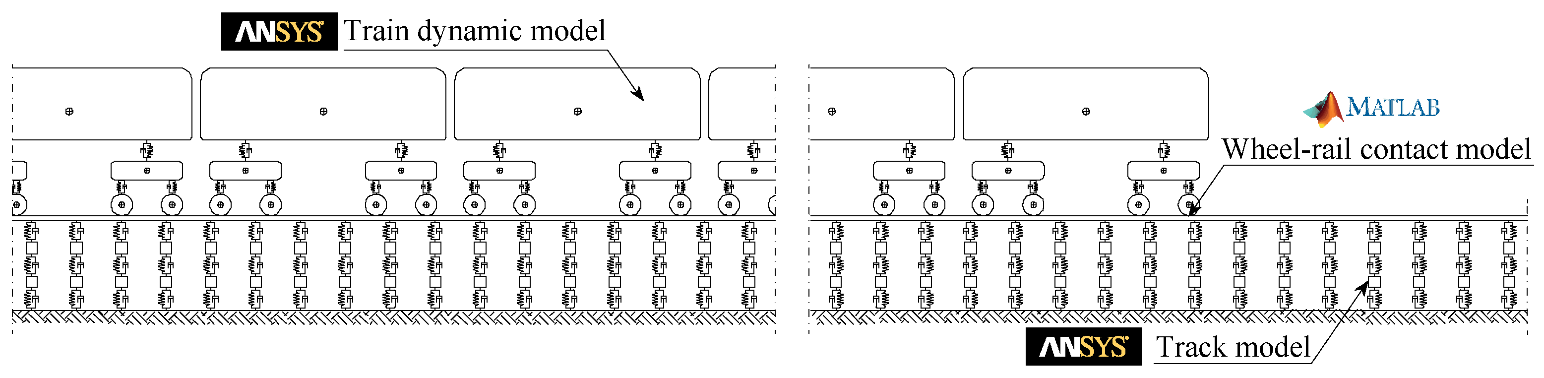
2. Train-Track Dynamic Interaction Modeling

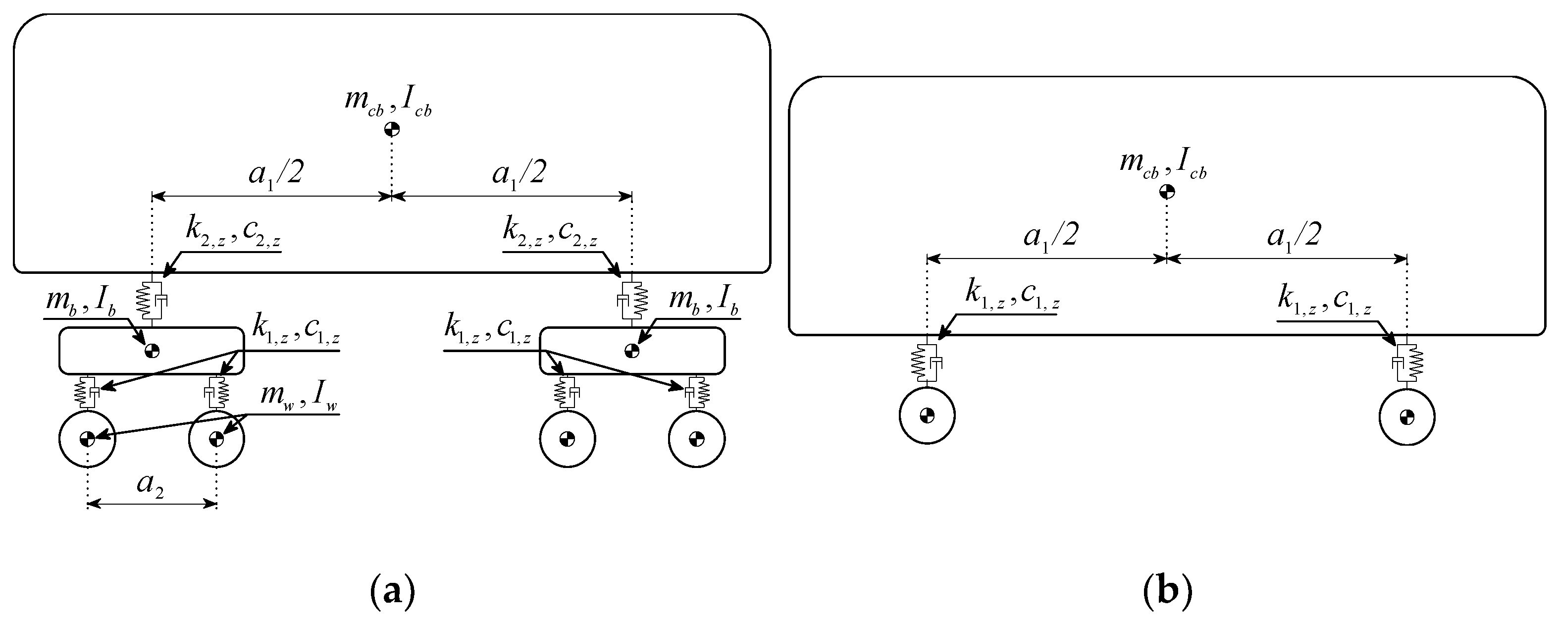
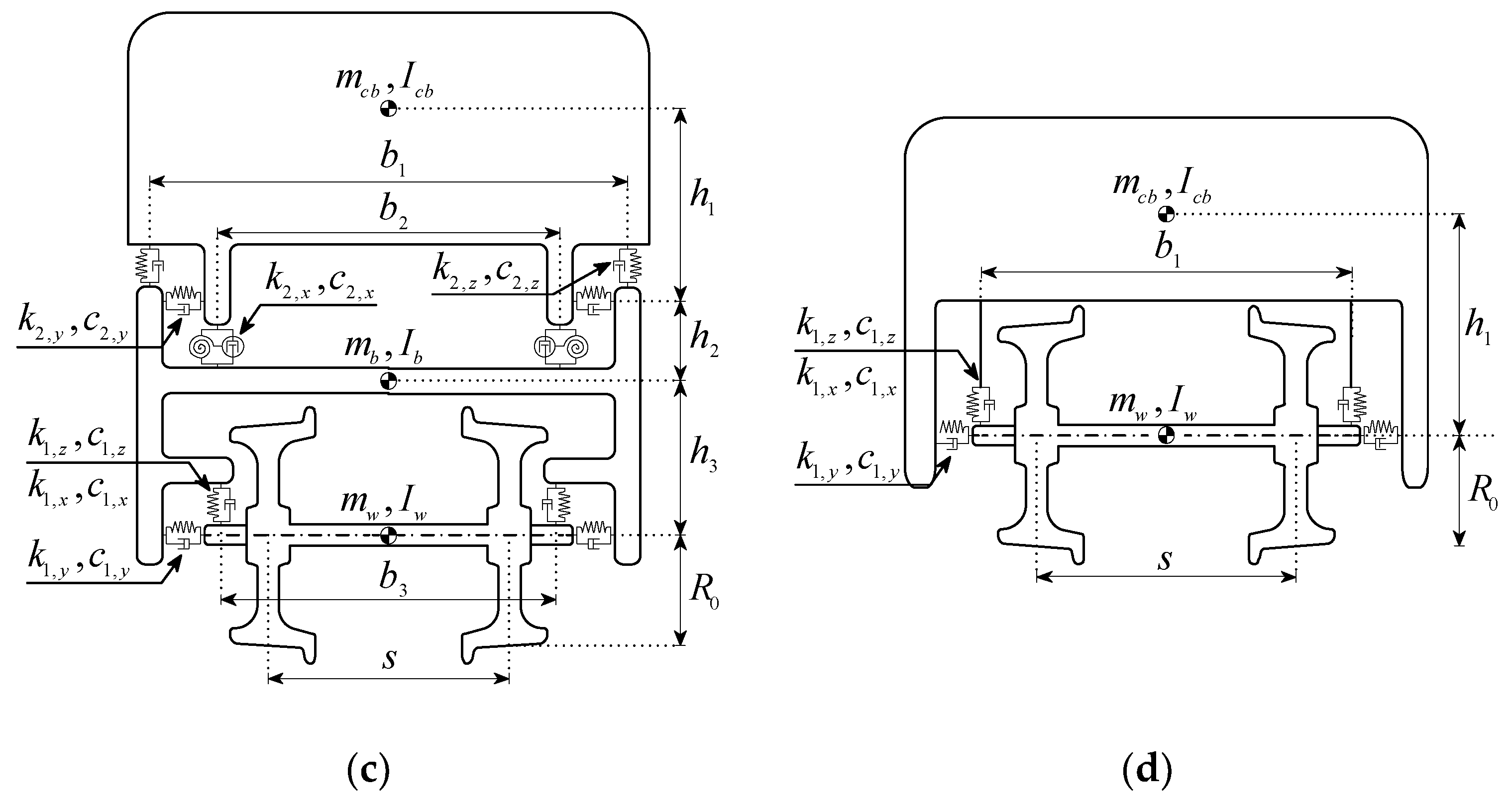
2.1. Numerical Modeling for Alfa Pendular Vehicle and Freight Wagon

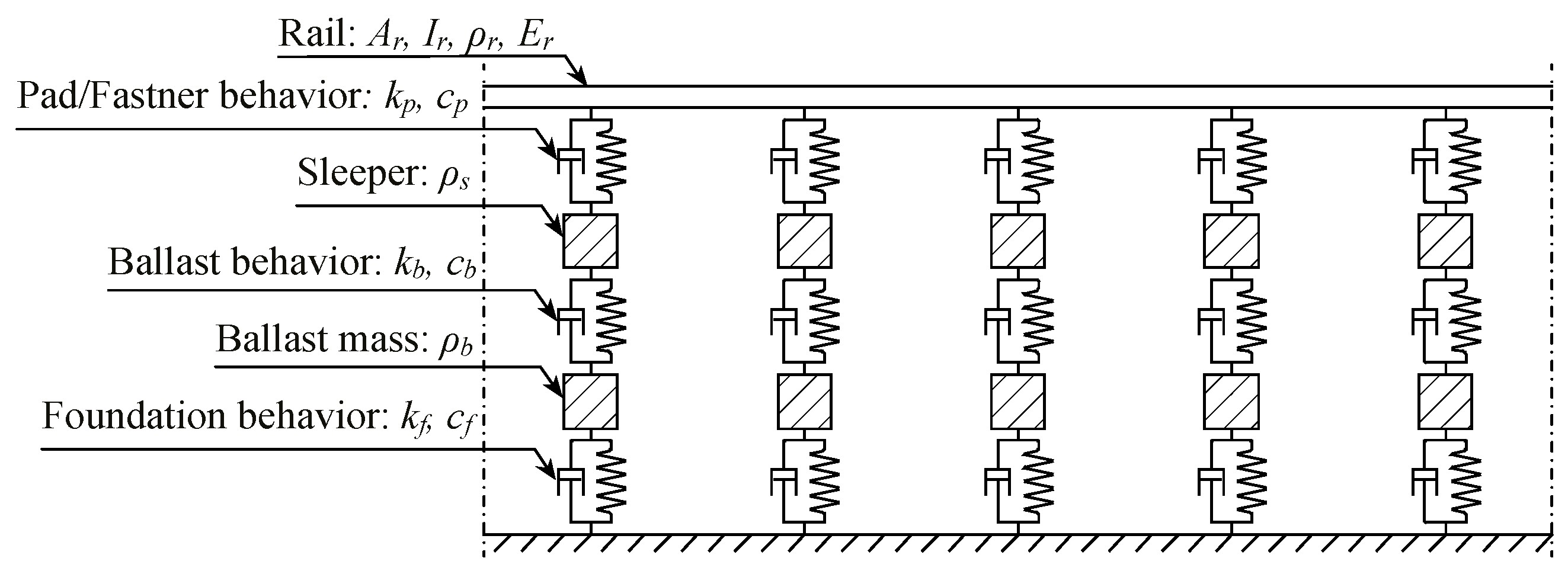
In order to enhance the parametric study carried out in the present paper, two different train models were developed, namely a passenger (Alfa Pendular) train and a container freight (Laagrss wagon). The numerical models of both trains were performed in the Finite Element Method (FEM) package ANSYS^® [38] using spring-damper elements COMBIN14 to simulate the suspensions that connect the various components of the trains, including car body, bogies, and wheelsets. The mass and the rotary inertia of the mentioned components are taken into account through mass point elements MASS21. The dynamic models adopted for each train are depicted in Figure 1. As presented in this figure, k, c, m, and I denote stiffness, damping, concentrated mass, and rotary inertia. Moreover, the subscripts c_b, b, and w refer to the car body, bogies, and wheelsets. r_w is the wheel radius, and gauge is indicated by s. Finally, the characters a, b, and h denote the longitudinal, transversal, and vertical distances. The geometrical and mechanical properties of both trains are presented in

Table 1. Parameters for the Alfa Pendular vehicle (adapted from Neto et al. (2020) [39]).

Parameter	Value
Car body mass, mcb	35,640 kg
Car body roll moment of inertia, Icb,x	55,120 kg·m2
Car body pitch moment of inertia, Icb,y	1,475,000 kg·m2
Car body yaw moment of inertia, Icb,z	1,477,000 kg·m2
Bogie mass, mb	2829 kg
Bogie roll moment of inertia, Ib,x	2700 kg·m2
Bogie pitch moment of inertia, Ib,y	1931.49 kg·m2
Bogie yaw moment of inertia, Ib,z	3878.76 kg·m2
Wheelset mass, mw	1711 kg
Wheelset roll moment of inertia, Iw,x	733.4303 kg·m2
Wheelset yaw moment of inertia, Iw,z	733.4303 kg·m2
Stiffness of the primary longitudinal suspension, k1,x	44,981,000 N/m
Stiffness of the primary transversal suspension, k1,y	30,948,200 N/m
Stiffness of the primary vertical suspension, k1,z	1,652,820 N/m
Damping of the primary vertical suspension, c1,z	16,739 N·s/m
Stiffness of the secondary longitudinal suspension, k2,x	4,905,000 N/m
Stiffness of the secondary transversal suspension, k2,y	2,500,000 N/m
Stiffness of the secondary vertical suspension, k2,z	734,832 N/m
Damping of the secondary longitudinal suspension, c2,x	400,000 N·s/m
Damping of the secondary transversal suspension, c2,y	17,500 N·s/m
Damping of the secondary vertical suspension, c2,z	35,000 N·s/m
The static load transmitted by each wheel	64,000 N
Longitudinal distance between bogies, a1	19 m
Longitudinal distance between wheelsets, a2	2.7 m
Transversal distance between vertical secondary suspensions, b1	2.144 m
Transversal distance between longitudinal secondary suspensions, b2	2.846 m
Transversal distance between primary suspensions, b3	2.144 m
Vertical distance between car body center and secondary suspension, h1	0.936 m
Vertical distance between bogie center and secondary suspension, h2	0.142 m
Vertical distance between bogie center and wheelset center, h3	0.065 m
Nominal rolling radius, rw	0.43 m
Gauge, s	1.67 m

and

Table 2. Parameters for the freight wagon (adapted from Neto et al. (2019) [40]).

Parameter	Value
Car body mass, mcb	41,100 kg
Car body roll moment of inertia, Icb,x	48,997.023 kg·m2
Car body pitch moment of inertia, Icb,y	673,322.463 kg·m2
Car body yaw moment of inertia, Icb,z	665,107.6 kg·m2
Wheelset mass, mw	1246.52 kg
Wheelset roll moment of inertia, Iw,x	311.839 kg·m2
Wheelset yaw moment of inertia, Iw,z	311.839 kg·m2
Stiffness of the longitudinal suspension, k1,x	44,981,000 N/m
Stiffness of the transversal suspension, k1,y	30,948,200 N/m
Stiffness of the vertical suspension, k1,z	1,860,000 N/m
Damping of the vertical suspension, c1,z	16,739 N·s/m
The static load transmitted by each wheel	107,000 N
Longitudinal distance between wheelsets, a1	6 m
Transversal distance between vertical suspensions, b1	2.17 m
Vertical distance between car body center and suspension, h1	1.867 m
Nominal rolling radius, rw	0.43 m
Gauge, s	1.67 m

. Note that in all analyses, only one car was taken into account to simplify the numerical computations.

2.2. Railway Track

The numerical model of the track was developed in ANSYS^® [38] and is schematized in Figure 2. It consists of a three-layer model composed by the rail modeled with beam elements BEAM181, and by the ballast and sleepers modeled with mass point elements MASS21. These three layers are connected through linear spring-damper elements COMBIN14, which simulate the foundation, the ballast and the pad/fastener, indicated in Figure 2 by the subscripts f, b, and p, respectively. The mechanical properties of the different elements are presented in

Table 3. Mechanical properties of the track.

Parameter		Value
Rail	Ar (m2)	7.67 × 10−4	[41]
	ρr (kg/m3)	7850	[41]
	Ir (m4)	30.38 × 10−6	[41]
	νr	0.28	[41]
	Er (N/m2)	210 × 109	[41]
Rail pad, longitudinal	Kp (N/m)	20 × 106	[42]
	Cp (N·s/m)	50 × 103	[42]
Rail pad, lateral	Kp (N/m)	20 × 106	[42]
	Cp (N·s/m)	50 × 103	[42]
Rail pad, vertical	Kp (N/m)	500 × 106	[43]
	Cp (N·s/m)	200 × 103	[43]
Sleeper	ρs (kg/m3)	2590
	νs	0.2
	Es (N/m2)	40.9 × 109
Ballast, longitudinal	Kb,x (N/m)	9000 × 103	[44]
	Cb,x (N·s/m)	15 × 103	[45]
Ballast, lateral	Kb,y (N/m)	2250 × 103	[46]
	Cb,y (N·s/m)	15 × 103	[45]
Ballast, vertical	Kb,z (N/m)	30 × 106	[46]
	Cb,z (N·s/m)	15 × 103	[45]
Foundation, longitudinal	Kf,x (N/m)	20 × 106	[47]
	Cf,x (N·s/m)	5.01 × 102	[47]
Foundation, lateral	Kf,y (N/m)	20 × 106	[47]
	Cf,y (N·s/m)	5.01 × 102	[47]
Foundation, vertical	Kf,z (N/m)	20 × 106	[47]
	Cf,z (N·s/m)	5.01 × 102	[47]

.

In real conditions, the rails are not perfect, which also affects the wheel-rail forces. Therefore, a sample of the track irregularity was measured on a Northern Line of the Portuguese Railway Network as the initial excitation of the wheel-rail contact. More details about the unevenness profile measurement are provided by Mosleh et al. [25]. As an example, Figure 3 depicts a 220 m stretch (the total length of the simulation) of the vertical and lateral irregularity profiles corresponding to the right rail. The sample of the track irregularity profile shown in Figure 3 is used for all analyses in this research study.

2.3. Train-Track Interaction

The train-track dynamic interaction coupling system is solved using the numerical tool “VSI-Vehicle-Structure Interaction Dynamic Analysis.” This tool is based on the Lagrange multipliers method, in which the constraint equations that relate the train displacements with the nodal displacements of the track, including the track irregularities, are added to the equilibrium equations, forming a single system that defines the coupling between the two sub-structures. Note that when including the track irregularities in the constraint equations, it is not necessary to include them explicitly in the FEM model, which considerably simplifies the analysis. Moreover, as will be mentioned later, it is also possible to include the wheel flats as a periodic rail irregularity. To solve the train structure detachment, Neves et al. [48] and Montenegro et al. [49] extended the original formulation developed by Neves et al. [50]. Subsequently, Montenegro et al. [51] reformulated the method to consider the lateral interaction by taking into account the wheel and rail geometry and the contact model between them. In the last upgrade, the vertical and lateral contact forces were computed and made the software possible to deal with different scenarios.

The wheel-rail contact model adopted in this numerical tool has been validated with numerical examples and experimental data (see [48,51]) and is based on a specially developed finite contact element that considers the geometry of the contact interface by parameterizing the wheel and rail profiles with cubic splines. The element uses the Lagrange multipliers method to guarantee the coupling between the vehicle and the track structure when contact occurs, but can also lead to wheel-rail detachment. The contact formulation implemented in this contact element can be defined by three main steps, namely: (i) the geometric analysis, (ii) the normal contact analysis, and (iii) the tangential contact analysis.

The geometric analysis consists of evaluating the location of the contact points between the wheel and the rail based on the geometry of their profiles previously parameterized through cubic splines. The contact search is then carried out through a couple of nonlinear equations, whose solution guarantees the compatibility between the two contacting bodies (see [51] for details). Although the present study does not focus on scenarios with important lateral loads, it is important to highlight that the wheel profile is parameterized by two surfaces (tread and flange), which enables the algorithm to deal with double contact point scenarios where the flange also touches the rail.

With the location of the contact points determined, the computation of the contact forces through the normal and tangential contact algorithms can then be performed. The former is based on the Hertz nonlinear theory [52] and aims to compute the contact forces perpendicular to the contacting bodies, while the latter uses Kalker’s USETAB [53] routine to calculate the creep forces that arise from the rolling friction contact between the wheel and the rail.

The dynamic coupling formulation used in this work, and schematized in Figure 4, is programmed in MATLAB^® [54], which imports the structural matrices of the track and the train modeled in the FEM package ANSYS^® [38]. A detailed description of the interaction model, as well as its validation, can be found in Montenegro et al. [51] and Montenegro [55]. Figure 4 presents the modeling of train-track interaction numerical modeling.

2.4. System Description

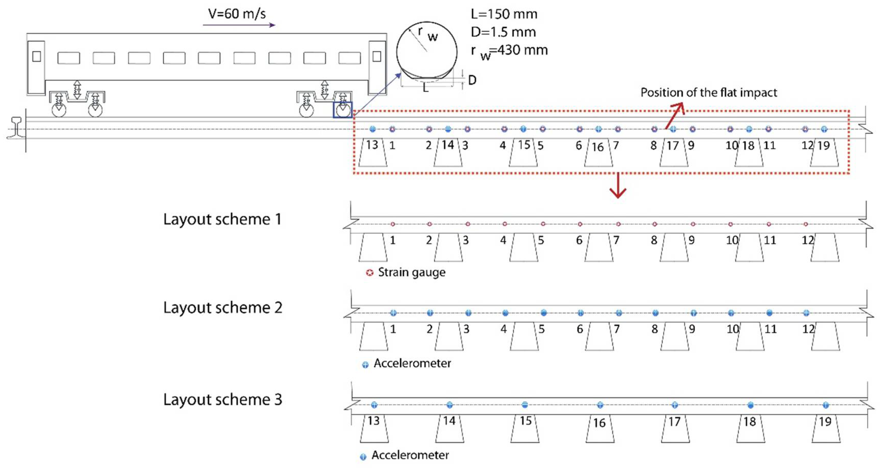
2.4.1. Layout Scheme of Multisensor Arrays

The wheel flat detection system consists of a range of strain gauges (SGs) and accelerometers installed along a stretch of the track. The shear and accelerations are evaluated for the 19 positions of the track illustrated in Figure 5, which represent the positions where the sensors would be installed in a real wayside system. In this figure, numbers 1 to 12 represent shear measurement or acceleration points, which simulate the position of the strain gauges (layout scheme 1) or accelerometers (layout scheme 2) installed on the rail, while numbers 13 to 19 represent only acceleration measurement points (layout scheme 3), which represent the position of the accelerometers installed on the rail over the sleepers.

Although strain gauges are widely used in field tests for the experimental evaluation of wheel-rail forces, they are not suitable for long-term monitoring of wheel flats, as they are vulnerable to electromagnetic interference from environmental conditions. Moreover, base drift for strain gauges is unavoidable during long-term service, making it impossible to maintain consistency for a long period. For these reasons, and unlike the previous work carried out by Mosleh et al. [37], in which only shear responses were considered to detect wheel flats, a parametric study was performed to compare the accuracy of the system using acceleration responses. The wheel flat was identified through the envelope spectrum approach by considering the evaluated shear and the accelerations as inputs. The results were compared considering different track responses to determine the precise wheel flat due to the type and position of the sensors and the wheel flat level.

2.4.2. Flat Geometry

Figure 5 presented a vehicle passing through the virtual sensors. The front wheel of the vehicle has a defect with the following characteristics: wheel flat length (L) is 150 mm and flat depth (D) is 1.5 mm. The impact of the wheel flat occurred before position 9. The speed of the vehicle is 60 m/s. The wheel flat vertical profile deviation is defined as:

$$Z=-\frac{D}{2}\left(1-cos\frac{2\pi x}{L}\right)H\left(x-\left(2\pi r_w-L\right)\right), 0\le x\le 2\pi r_w$$

(1)

where $D$ is the depth of the flat, $L$ is the length of the flat, $r_w$ is the radius of the wheel, and H represents the Heaviside function.

When a defective wheel rotates, a periodic impulse occurs due to the wheel flat that is applied to the track by the wheel at a specific frequency. After determining the wheel perimeter ($r_W$) and the speed of the vehicle ($S$), the frequency of the periodic impulse referring to the flat impact frequency can be calculated as follows:

$$f_f=\frac{S}{\left(2\pi r_W\right)}$$

(2)

The wheel flat is incorporated in the unevenness profile of the track defined in Figure 3 as a periodic irregularity with the shape given by Equation (1).

3. Methodology for Flat Detection

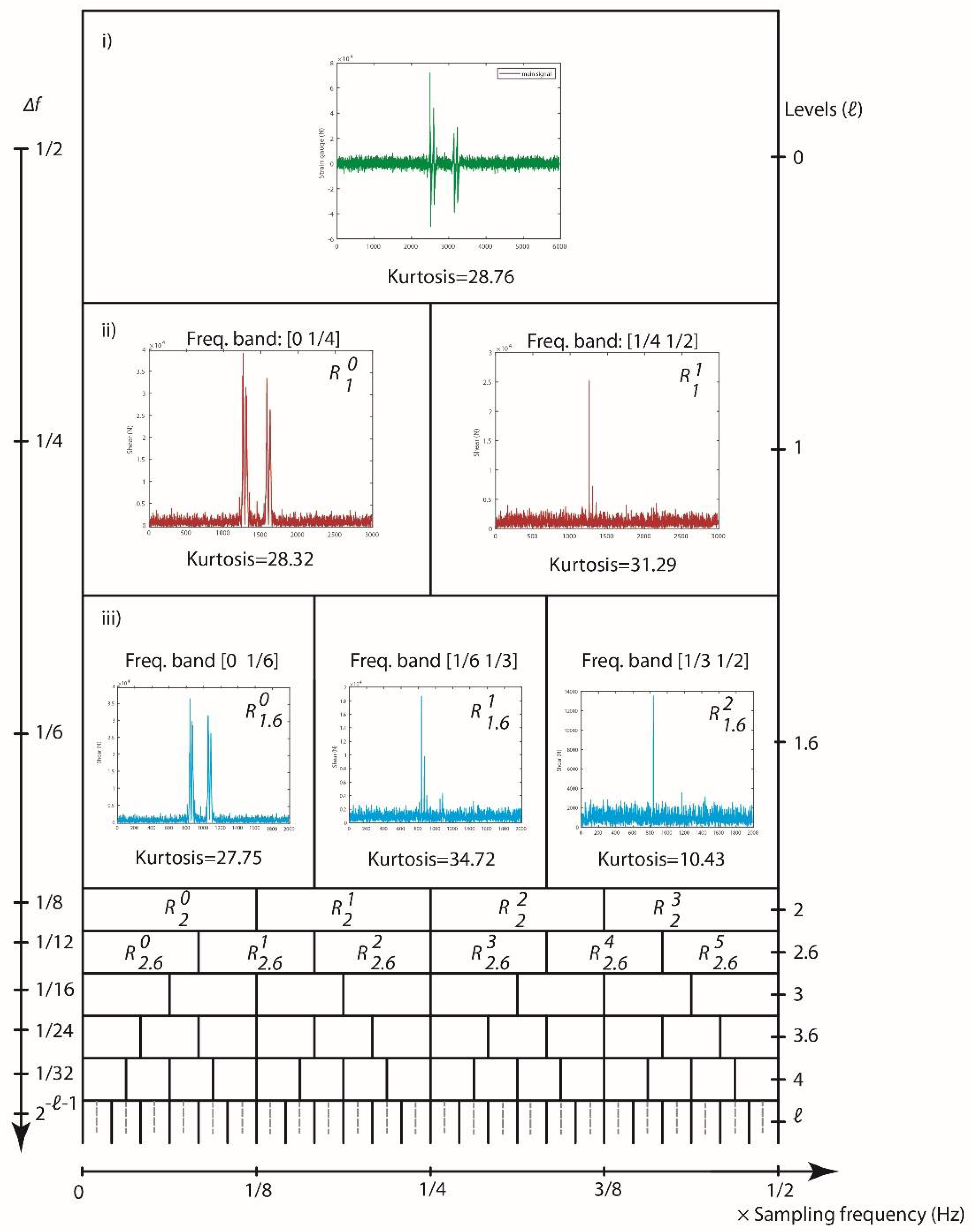
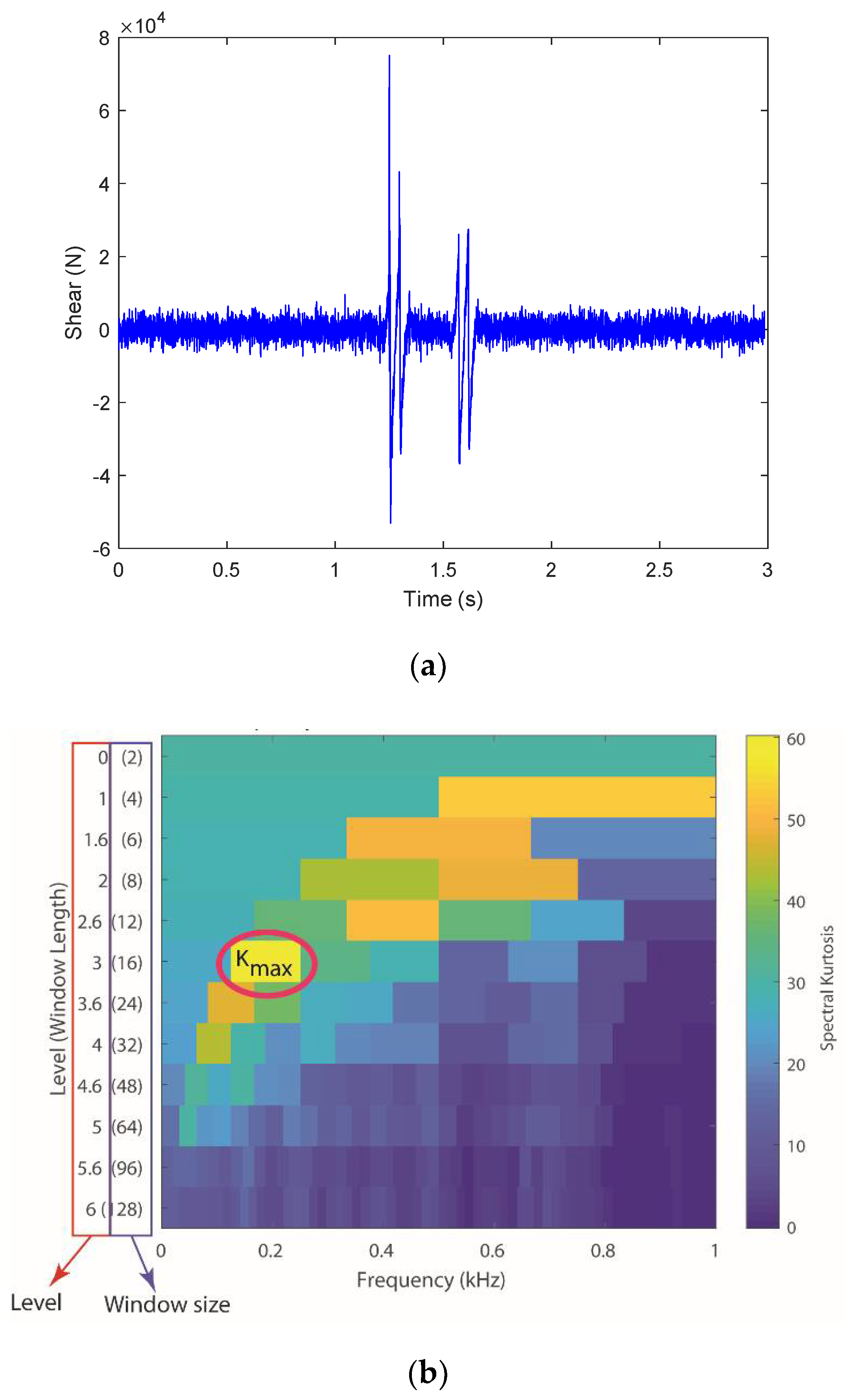
3.1. Definition of Kurtosis

The shape and density of the signal distribution can be visualized by moments about the mean [56]. The mean of a set of data ${\overline{x}}_m$, is calculated through the following equation:

$${\overline{x}}_m=\frac{1}{N}{\displaystyle \sum }_{j=1}^N{x}_i$$

(3)

in which $x_i$ is the recorded data sample and N is the number of samples. Therefore, the k-th central moment is calculated as:

$${\mu }_k=\frac{1}{N}{\displaystyle \sum }_{j=1}^N{\left(x_j-\overline{x}\right)}^k$$

(4)

where $\overline{x}$ is the true mean. Kurtosis is a non-dimensional quantity that measures the relative intensity of the signal compared to a Gaussian distribution. Signals with impulsive-type responses lead to high kurtosis values (K). It is defined as the fourth central moment (${\mu }_4$) divided by the square of variance ${\mu }_2^2$as follow [57]:

$$K=\frac{{\mu }_4}{{\mu }_2^2}$$

(5)

For signals containing impulse features, the kurtosis value can be high. Therefore, high amounts of kurtosis indicate that the data include spikes [58]. Since the defect in the wheel causes a spike in the signal, one way to detect the defect in the wheel is to calculate the kurtosis for various frequency bands rather than the original signal.

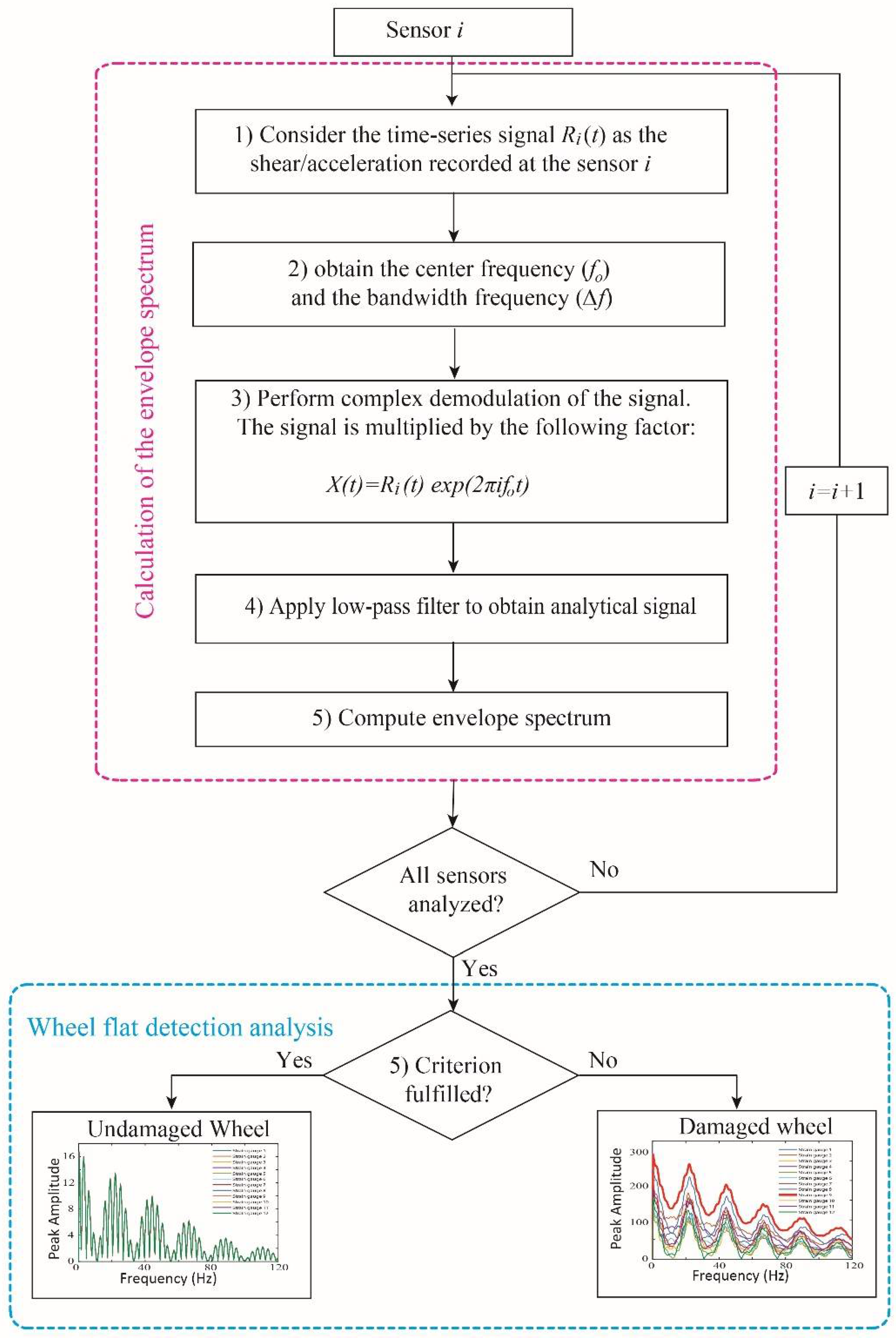
3.2. Envelope Spectrum Approach to Detect a Wheel with Spectral Kurtosis Analysis

Envelope spectrum detection is a technique to perform complex demodulation by shifting each frequency to zero and then applying a low-pass filter [59]. Therefore, the signal is multiplied by the following factor to perform a complex signal deformation.

$$X\left(t\right)=R\left(t\right)\exp \left(2\pi i{f}_{0}t\right)$$

(6)

where, $f_0$ is the center frequency of the band. After the frequency band with the highest kurtosis level is determined, a passband filter is applied to the raw signal to obtain a higher impulse signal to analyze the envelope spectrum. The process to identify a defective wheel is shown in Figure 6. As shown in this figure, the method to detect a wheel flat is presented with two main blocks. In the first block of the flowchart, the necessary equations for evaluating the envelope spectrum in each sensor of the installation system are explained, and furthermore, the wheel flat is identified in the second block based on the following criteria. If the responses obtained by all sensors are coincident, the amplitude of the envelope spectrum is the same and indicates the passage of a healthy wheel through the system. However, a significant lag in the amplitude of the envelope spectrum infers a passage of a defective wheel.

The selection of the demodulation band for the envelope analysis of a defective wheel is frequently performed by comparing the spectrum for a healthy wheel to select the particular frequencies at which the largest change occurred as a result of the fault. It has been identified that spectral kurtosis (SK) gives a very similar indication of the band to be demodulated without requiring historical data. The spectral kurtosis of a signal is obtained by dividing the main signal into different frequency bands and obtaining the kurtosis of each frequency band [60]. This demonstrates how the peak in the signal changes with frequencies and can be used to identify a frequency band within which a signal has the most impulsive behavior. This information is needed to select the optimal frequency band to demodulate and perform an envelope analysis on the recorded signals. The optimum center frequency and bandwidth combination of a bandpass filter to maximize the kurtosis of the filter output is described by a kurtogram [61].

The kurtogram shows the kurtosis results for a range of window lengths and frequencies and is used to visualize the spectral kurtosis. The principle of the proposed algorithm to obtain the kurtogram is based on the multirate filter-bank structure [60,61]. The algorithm is described first in the case of a binary tree structure and then extended to a 1/3-binary tree structure. The procedure to perform a kurtogram is described in the following steps:

• Time-series signal R(t) is considered, as the response recorded (shear or acceleration) in positions 1 to 19 (presented in Figure 5).
• Consider h as a low-pass prototype filter. Then construct two low-pass and high-pass analysis filters $h_1$and $h_2$, from h, in the frequency bands [0 $\frac{1}{4}$] and [$\frac{1}{4}$ $\frac{1}{2}$] of the sampling frequency, respectively, as follow:

  $$\begin{array}{c}{h}_1=h{e}^{j\pi /4}\\ h_2=h{e}^{j3\pi /4}\end{array}$$

  (7)

Filters $h_1$and $h_2$ are used to perform the low-pass/high-pass decomposition indicated in Figure 7, which is iterated in a pyramidal manner to produce the filter-bank tree, where each level has $2^l$ bands. As illustrated in this figure, let $R_l^i\left(t\right)$ be a sequence of coefficients issued from the filter i-th. $i$ is considered as $0,1,2,\dots ,2^{l-1}$ at each level ($l$) in the decomposition tree. After filtration, the main signal with $h_1$and $h_2,$ kurtosis values would be obtained for each signal.

3.

The idea of this step is to define three additional bandpass filters $g$ with frequency bands [0 $\frac{1}{6}$], [$\frac{1}{6} \frac{1}{3}$] and [$\frac{1}{3} \frac{1}{2}$] of the sampling frequency, as follow:

$$\begin{array}{c}{g}_1=g{e}^{j\pi /6}\\ g_2=g{e}^{j3\pi /6}\\ g_3=g{e}^{j5\pi /6}\end{array}$$

(8)

These filters are then used to further decompose each sequence $R_l^i\left(t\right)$ into three sub-sequences, regarding the low, medium, and high frequencies. After decomposition, the kurtosis of all these sub-sequences is computed according to Equation (5).

4.

After filtering with the above low-pass and bandpass filters, each signal obtained from section (ii) is taken into account as the main signal ($R_l^i\left(t\right)$) and this process is iterated from $l=0$ down to level $l-1$. The kurtogram would finally be estimated by computing the kurtosis for all sequence signals. The framework to obtain the kurtogram is depicted in Figure 7. Moreover, the center frequency and bandwidth frequency for the level with the highest kurtosis can be obtained by the following equations [60,61]:

$$\Delta f=2^{\left(-l-1\right)}{F}_s$$

(9)

$$f_o=\left(i+0.5\right)\Delta f$$

(10)

where $\Delta f$ is the bandwidth, $F_s$ is the sampling frequency, and $f_o$ is the center frequency.

Figure 8a shows a signal contaminated with noise obtained from position 9, considering layout scheme 1 (see Figure 5). Figure 8b presents the kurtogram using the above framework for the mentioned signal corresponding to the Alfa Pendular train.

As shown in Figure 8, the maximum kurtosis is obtained as 60.25 at level 3, with the corresponding band frequency equal to [$\frac{1}{16} \frac{1}{8}$]. Therefore, considering Equations (9) and (10), the center and bandwidth frequencies for the corresponding signal are calculated as follow:

$$\begin{array}{c}\Delta f=2^{\left(-3-1\right)}\times 2000=125\mathrm{Hz}\\ f_o=\left(1+0.5\right)\times 125=187.5\mathrm{Hz}\end{array}$$

(11)

where the sampling frequency ($F_s$) is 2000 Hz, the bandwidth frequency ($\Delta f$) is 125 Hz and the center frequency ($f_o$) is 187.5 Hz.

More details regarding the envelope spectrum approach for wheel flat detection are presented by Mosleh et al. [37]. In the following sections, the envelope spectrum approach is employed to detect a wheel flat. For this purpose, spectral kurtosis is used to calculate the center frequency and bandwidth for each signal as a key preprocessing step before performing the envelope spectrum. The sensitivity of the layout schemes (presented in Figure 5) is verified according to the type of sensors, the type of train, and the position of the sensors.

4. Sensitivity of Layout Schemes to the Unevenness Profile of the Rail and the Different Types of Trains

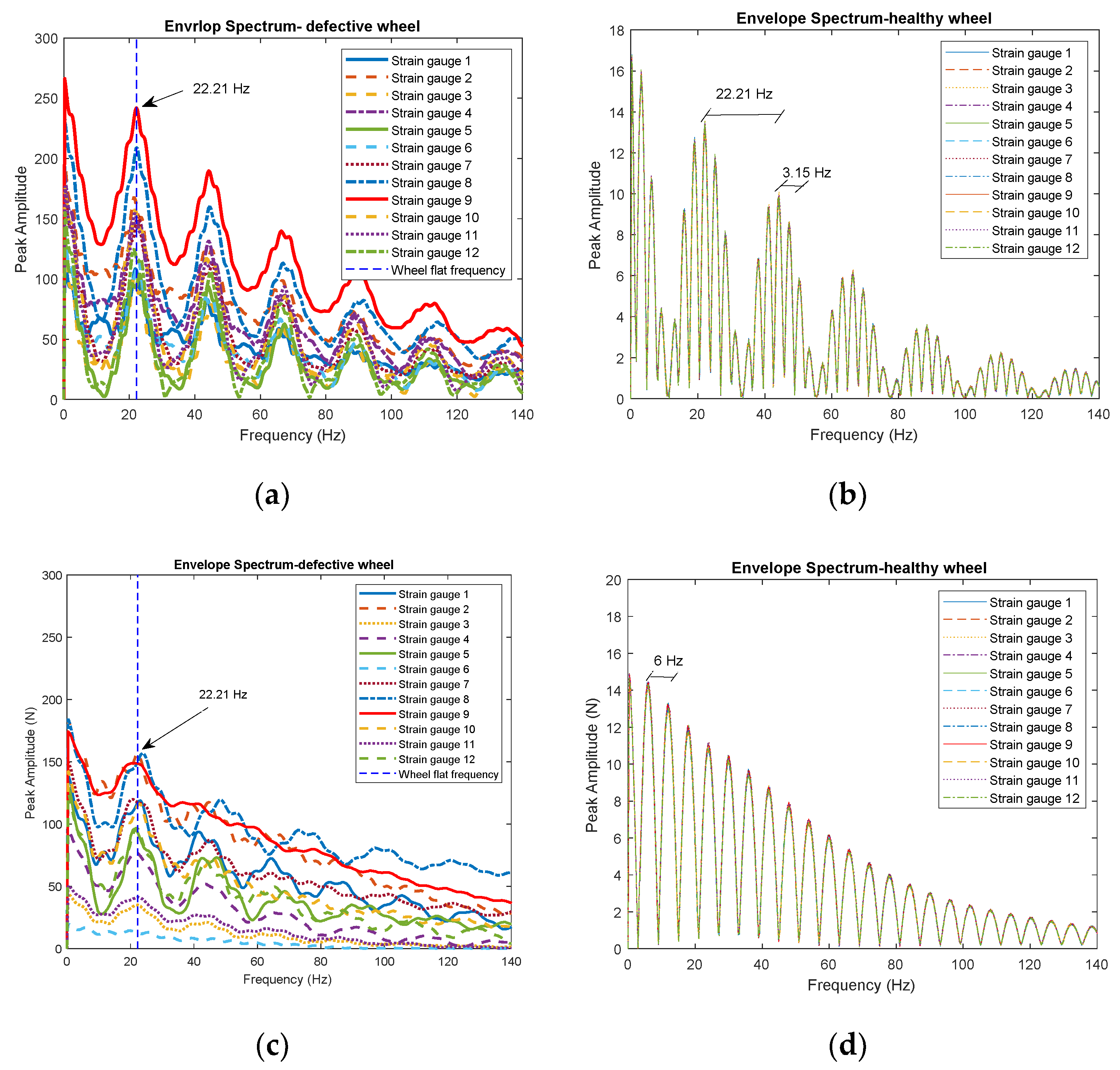
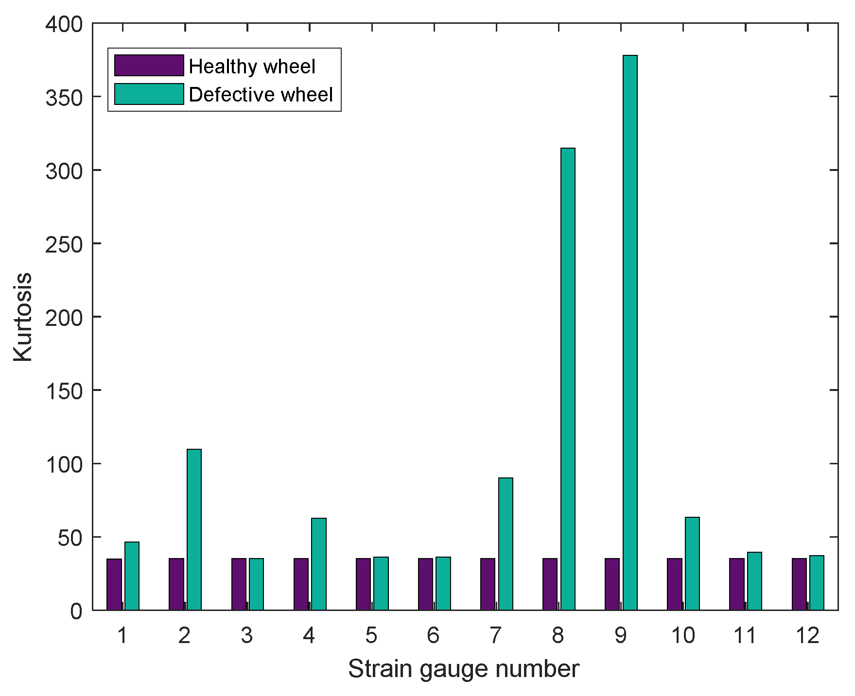
4.1. Track Response Obtained by the Strain Gauge Setup

The passage of one vehicle of the Alfa Pendular and a freight wagon in a track stretch with the irregularity profile presented in Figure 3 is investigated. In all analyses where a wheel flat is considered, only the right wheel of the first wheelset is damaged with this type of defect. As shown in Figure 5, the three layout schemes considered in this study aim to optimize the number and position of the sensors. As illustrated in this figure, layout scheme 1 includes 12 virtual strain gauges installed on the rail from a track stretch with a length equivalent to a wheel perimeter. The envelope spectrum approach is used to verify the sensitivity of layout scheme 1, considering the unevenness profile presented in Figure 3. The speed is considered as 60 m/s for both the Alfa Pendular and the freight wagon. Figure 9 presents the power spectrum of the envelope signal for the defective and healthy wheels corresponding to the 12 shear responses obtained on the rail (position 1 to 12 shown in Figure 5), due to the passage of the Alfa Pendular and freight wagon, considering the unevenness profile of the track. In the following figures, the vertical dash lines indicate the wheel flat frequency as 22.21 Hz.

By applying the envelop spectrum analysis, it is possible to observe a lag between the responses evaluated at the several SGs in the defective wheel, showing that a flat has been detected. On the other hand, as seen in Figure 9b,d, the responses in terms of the envelope spectrum in all SGs are very similar (no lag), indicating that there are no flats in both the Alfa Pendular and the freight wagon’s wheels. Moreover, the amplitude variation of the envelope spectral signal can also be seen as an additional indicator to evaluate whether the wheel is healthy or not. As shown in this figure, the amplitude variation of the envelope spectral signal of a defective wheel is higher than a healthy one.

The frequency content provides some interesting information. There are some high magnitude peaks corresponding to the bogies passing frequency (Figure 9b,d), which can be calculated as

$$f_b=\frac{S}{a_1}$$

(12)

where $f_b$ is the bogie frequency and $a_1$ is the regular spacing (see Figure 1), which for the Alfa Pendular corresponds to the spacing between bogies ($a_1$ = 19 m) and for the freight wagon, since it has no bogies, corresponds to the spacing between axles ($a_1$ = 6 m). Therefore, $f_b$was calculated as 3.15 and 6 Hz for the Alfa Pendular and the freight wagon, respectively. In other words, Figure 9b corresponds to the passage of the healthy wheel of the Alfa Pendular and presents the bogie passing frequency as 3.15 Hz and the wheel passing frequency as 22.17 Hz. However, in Figure 9a, corresponded to the passage of a defective wheel of the Alfa Pendular, only the frequency of the defective wheel (22.21 Hz) can be seen. Figure 10 shows the kurtosis values for healthy and defective wheels corresponding to 12 positions of the strain gauges (layout scheme 1) for the Alfa Pendular.

As presented in this figure, a signal corresponding to a defective wheel has significantly greater impulsiveness, especially for strain gauge 9, which is located after the wheel flat impact location. However, since the unevenness profile does not generate strong variations in the signal, compared to the flat wheel, all kurtosis values obtained for a healthy wheel are the same for the 12 signals.

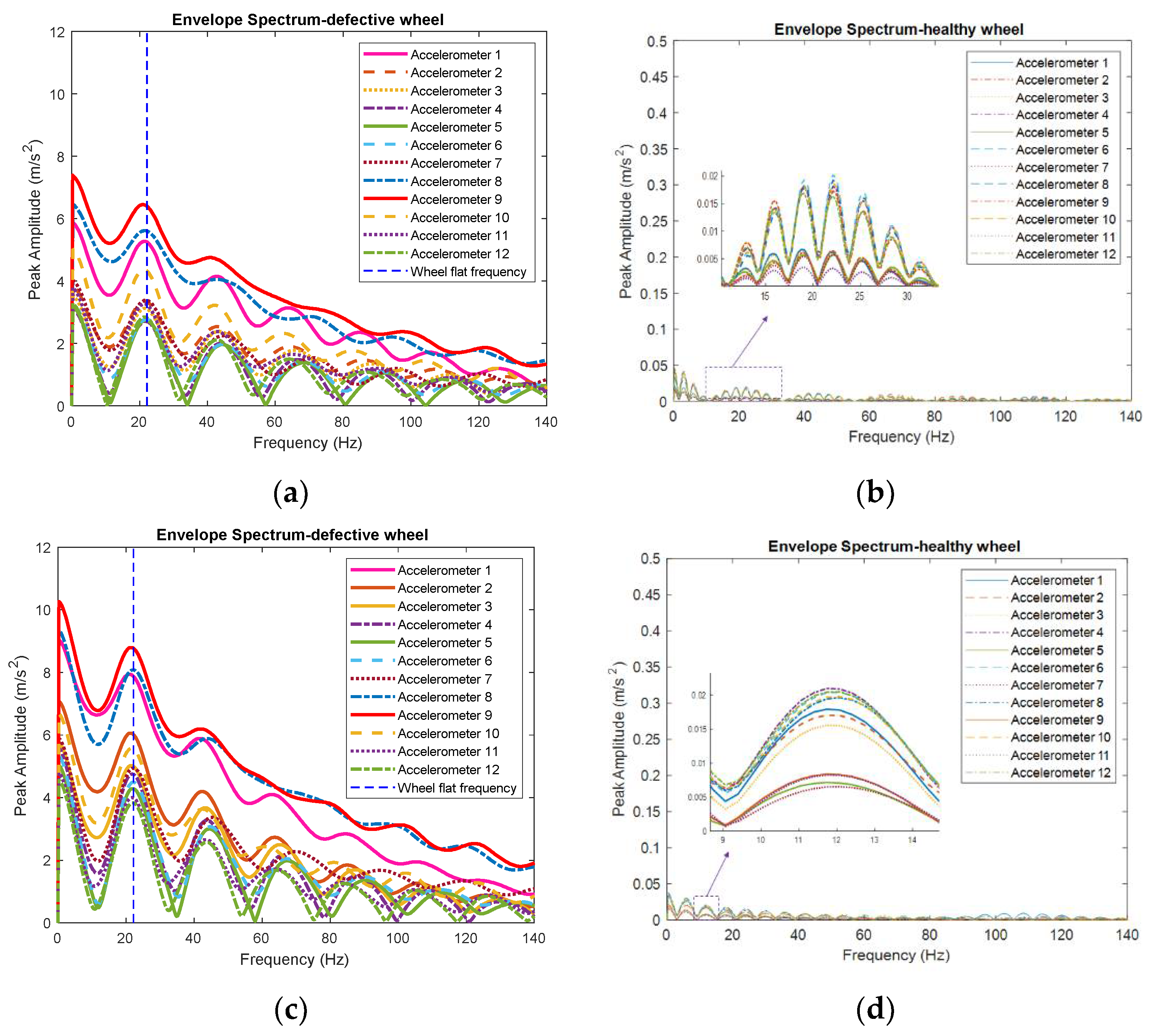
4.2. Track Response Obtained by the Accelerometers

The previous section has shown that the envelope spectrum approach is able to detect a defective wheel from a healthy one for 12 virtual strain gauges located in the rail (layout scheme 1). However, as mentioned above, the use of strain gauges for long-term monitoring of wheel flat is not suitable due to their vulnerability to water and electromagnetic interferences. To compare the track response of strain gauges and accelerometers, both were placed in the same location. This is shown in layout scheme 2, in Figure 5.

Figure 11 shows the envelope spectrum corresponding to the 12 acceleration responses obtained on the rail (position 1 to 12 shown in Figure 5) for the passage of the Alfa Pendular and the freight wagon, considering the track irregularities presented before. As for the SGs, it is possible to observe that, in the presence of a wheel flat, the responses of each accelerometer in terms of envelope spectrum present significant lag, while for the scenarios with a healthy wheel, this lag is practically insignificant. Moreover, the amplitude of the envelope spectral signal is also considerably different in the two situations, being much higher when the wheel is defective.

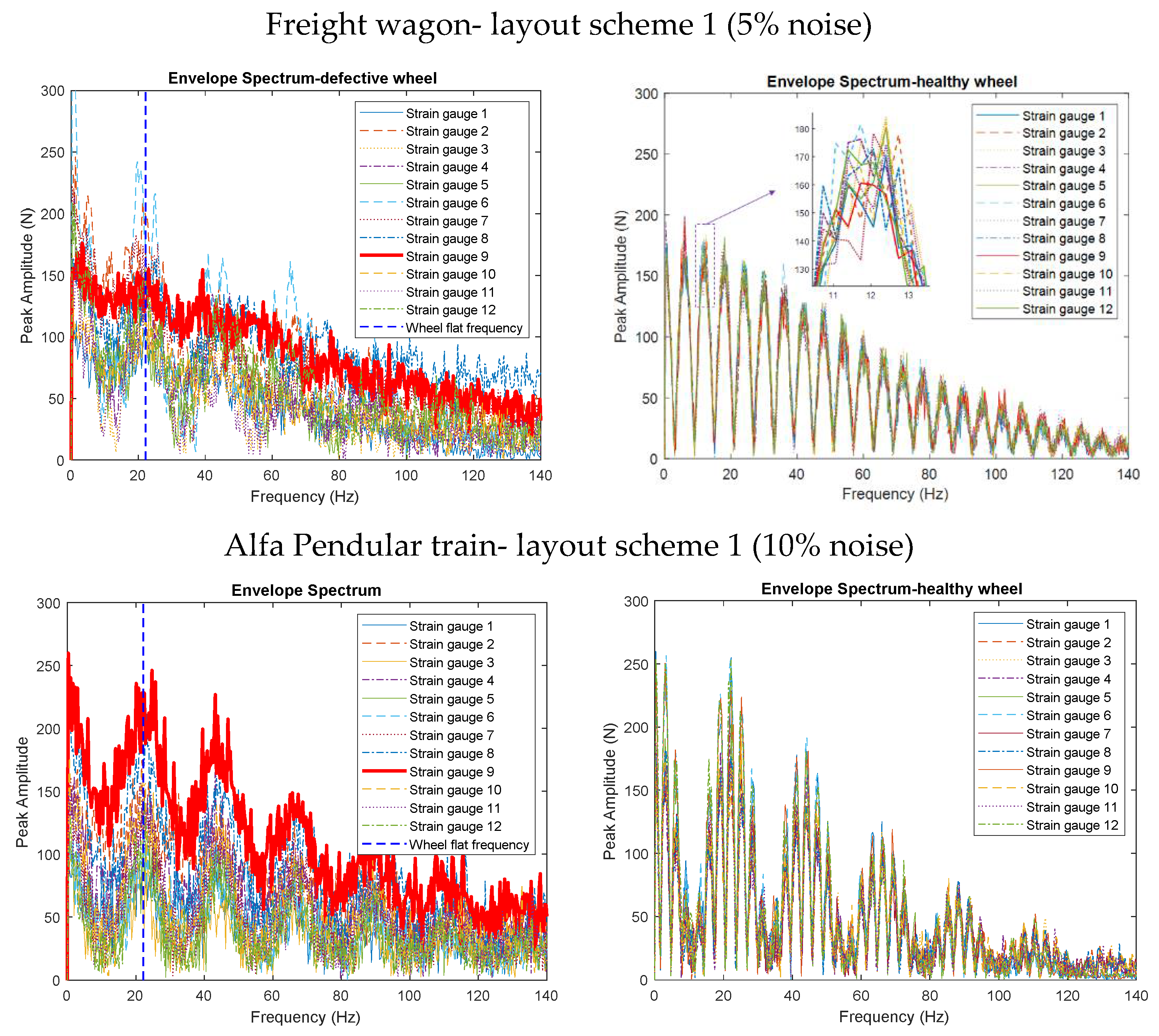
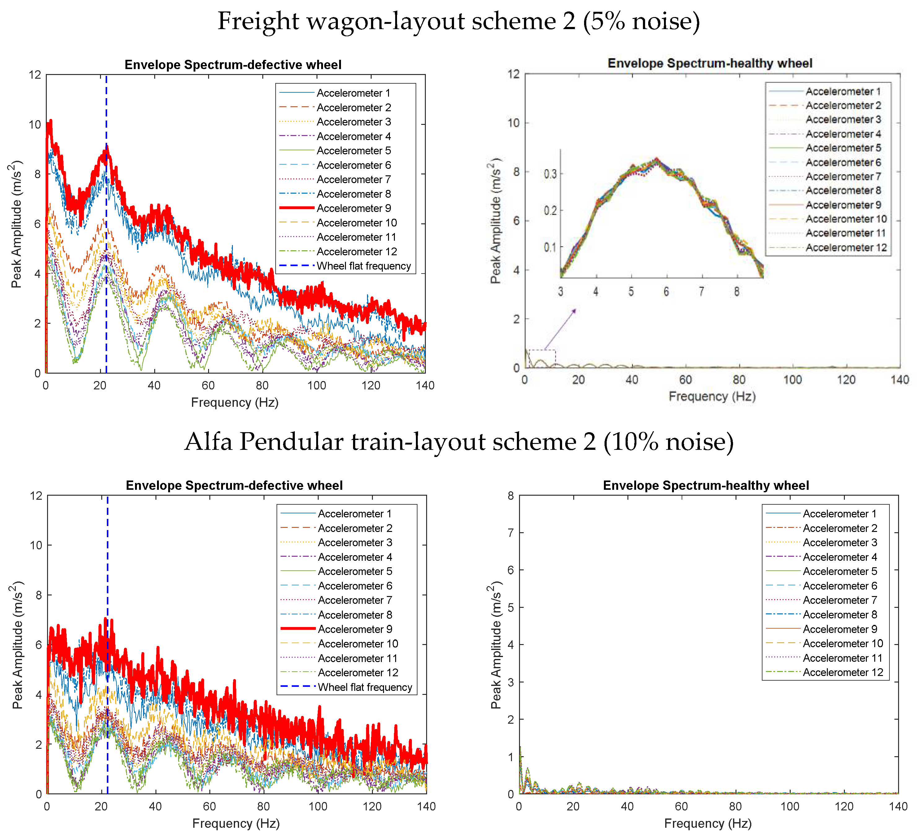
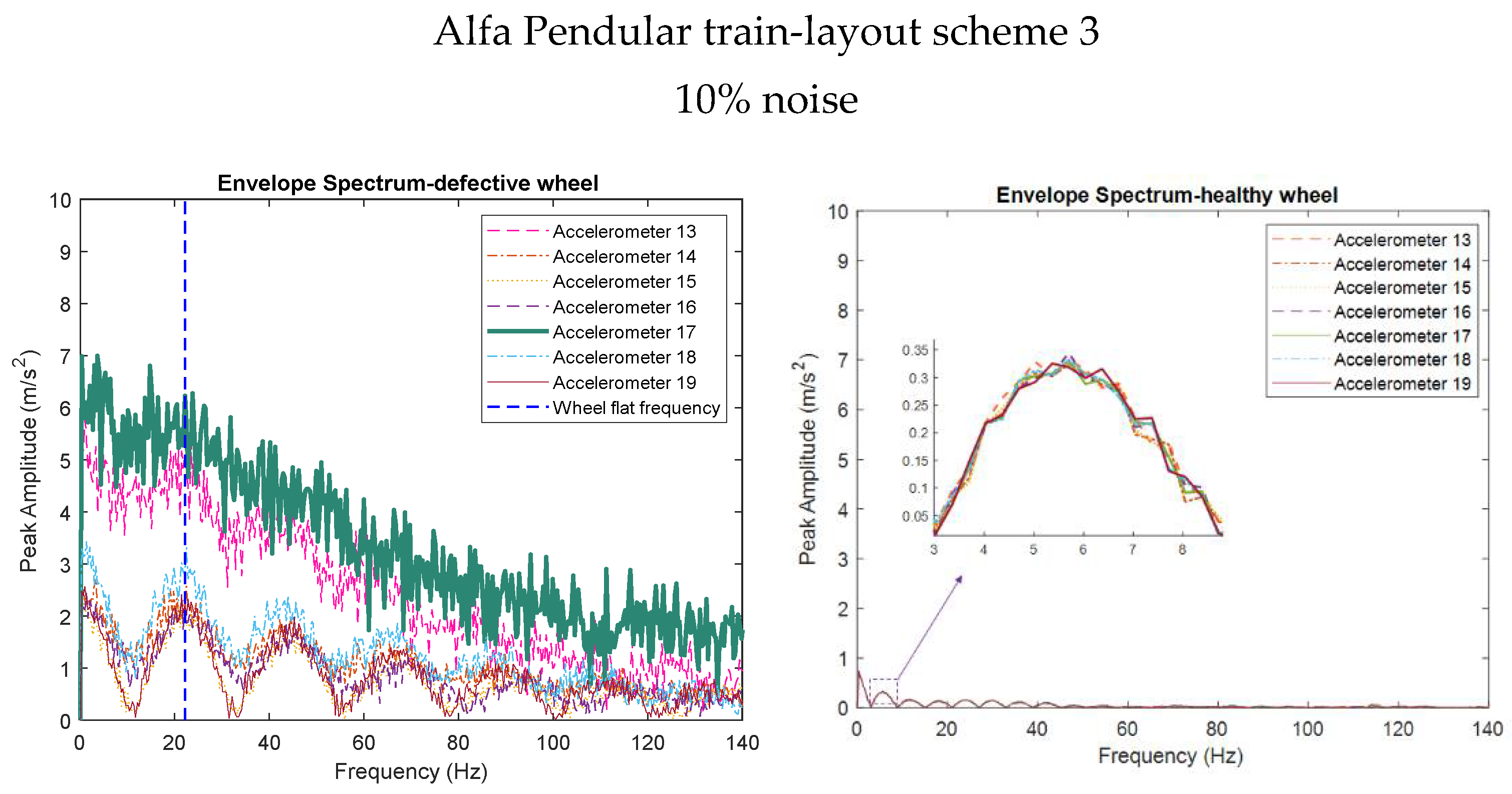
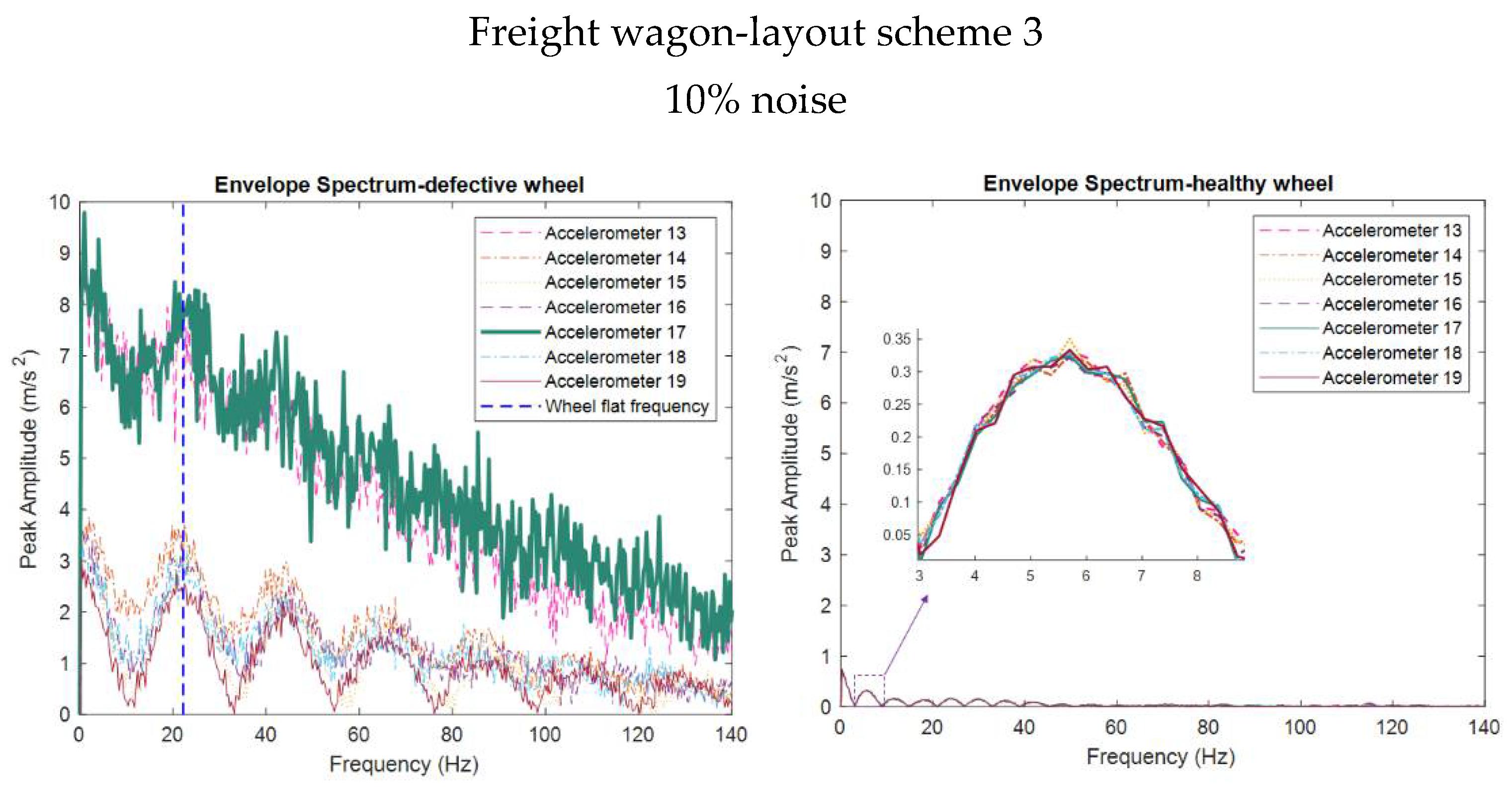
5. Sensitivity of the Layout Schemes to the Signal Noise

The signal noise can significantly perturb the assessment of the track response. To evaluate its influence in the proposed methodology to detect wheel flats, an artificial noise is generated due to the maximum response (shear or acceleration) of the signal and added to the main signal. Therefore, new signals considering different noise levels of 5%, 10%, and 20% of the maximum amplitude of the initial signal are generated. The unevenness profile of the track (presented in Figure 3) is considered. Moreover, the effectiveness of using shear and acceleration as input parameters for flat detection is compared, with respect to strain gauges (layout scheme 1) and accelerometers (layout scheme 2), considering the Alfa Pendular and the freight wagon.

Figure 12 and Figure 13 show an envelope spectrum detection analysis for 12 shear and acceleration responses obtained on the rail (position 1 to 12 shown in Figure 5) for different noise intensities and considering a defective and a healthy wheel of the Alfa Pendular train and the freight wagon. As mentioned before, there are usually two indicators that can be used to detect wheel flats, namely the lag between signals and the amplitude value. It can be observed that the first one can also be used in the present scenario since a clear lag between the signals in the presence of a wheel flat is observed, while in the healthy wheel, all signals coincide. However, when looking at the amplitudes of the signals, it is possible to conclude that this indicator is not suitable when the shear is considered as input. In other words, when the signal is contaminated by noise and track responses evaluate by SGs, the only indicator that effectively distinguishes a defective from a healthy wheel is the clear lag between the amplitude of the envelope spectrum obtained with different sensors. On the other hand, the use of accelerometers is clearly more beneficial than using strain gauges to perform an envelope spectrum analysis for the detection of defective wheels, since the amplitude observed in the scenario with defective wheel scenario is considerably higher than that obtained with a healthy wheel, making the amplitude indicator also suitable when using this kind of layout scheme.

As demonstrated in a previous study [37], the time-domain response is not suitable to distinguish a healthy from a defective wheel due to the noise contamination of the signal. Therefore, some signal processing is required to extract fault detection under this situation. Figure 14 shows the kurtosis values for signals with and without noise for the Alfa Pendular passage for layout scheme 2. As presented in this figure, the noise-free signal is significantly more impulsive, causing the envelope spectrum analysis to effectively detect the fault. As an example, regarding accelerometer 9, when the signal is not marked by noise, the kurtosis value is approximately 2400.

When a 20% noise contamination is imputed to the signal, the kurtosis value decreases to 400 in relation to the noise-free signal, but the pattern remains constant, and the maximum kurtosis value corresponds to accelerometer 9, which is closer to the impact of the flat. This means that the framework is effective even when the noise-to-signal ratio is high.

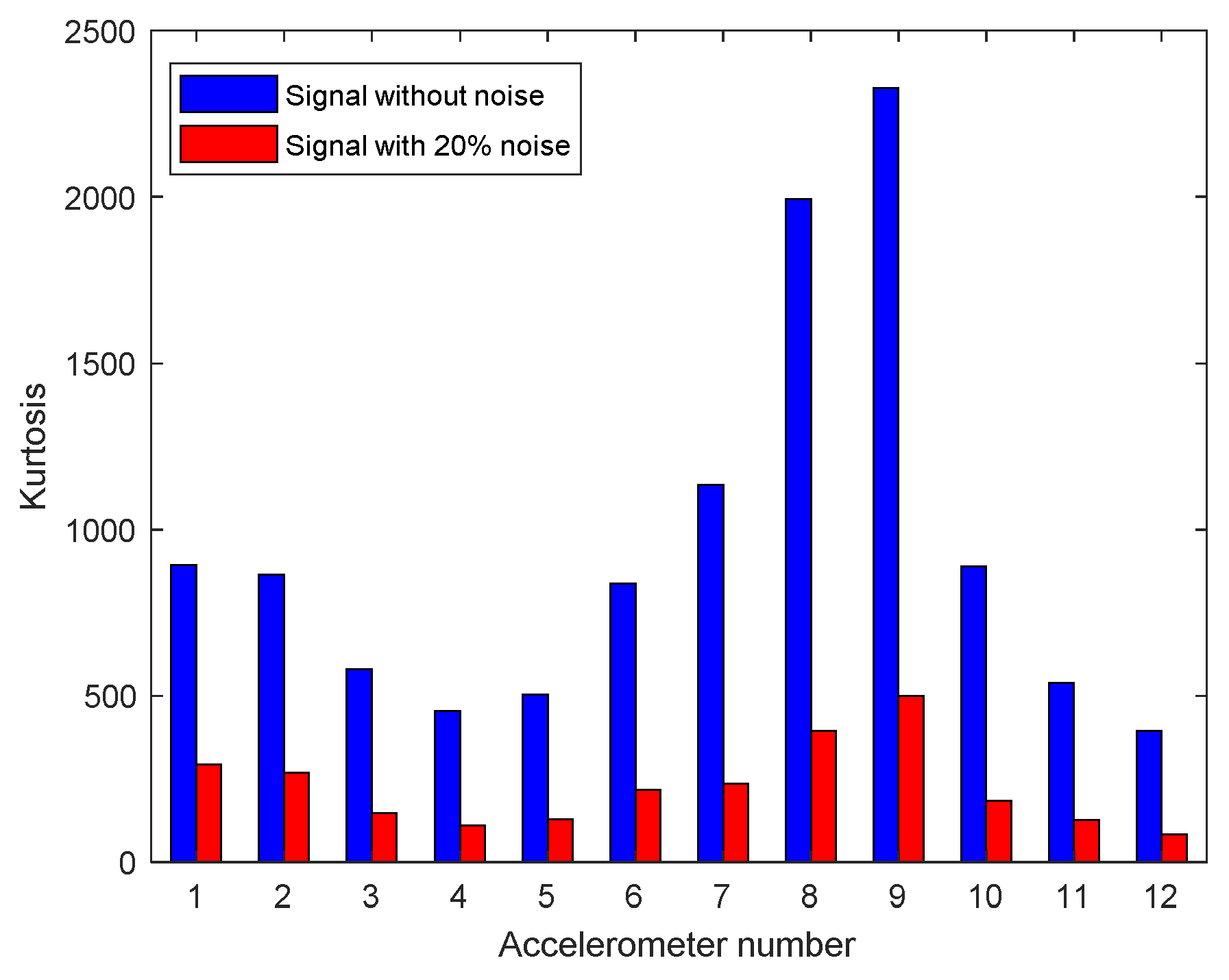
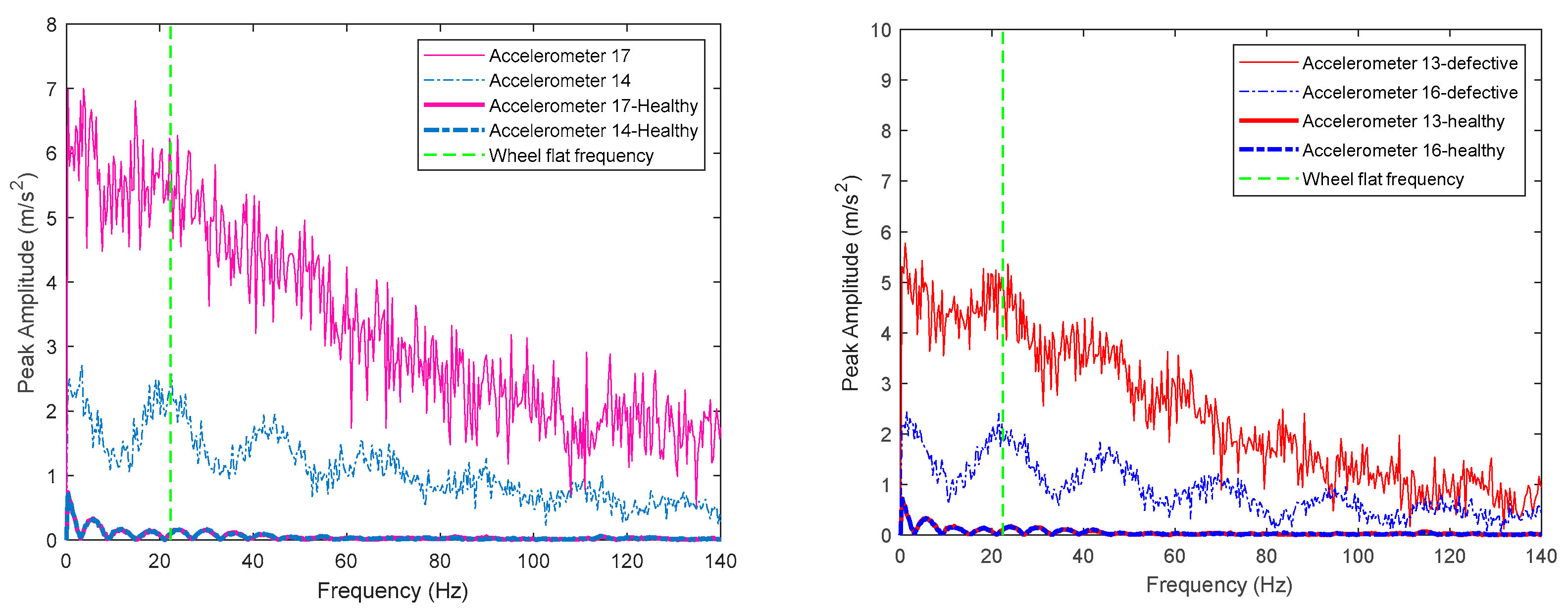
6. Sensitivity of the Layout Schemes to the Number and Location of the Accelerometers

As stated above, in order to reduce installation and maintenance costs, it is of the utmost importance to reduce the number of sensors without compromising the quality of the output results. Moreover, it is important to demonstrate that the system, regardless of the position of the sensors, is always effective in detecting wheel flats. Therefore, this section aims to demonstrate the sensitivity of the layout schemes to the number of sensors (strain gauges or accelerometers) and the location where they are installed. Consequently, in addition to the 12 positions selected on the rail between the two sleepers, seven more accelerometers (positions 13 to 19 shown in Figure 5) were considered on the rail located above each sleeper (layout scheme 3). The robustness of the proposed method for detecting a wheel flat with fewer sensors without compromising data quality is discussed in this section.

Figure 15 shows the envelope spectrum detection analysis for seven accelerometers (positions 13 to 19 shown in Figure 5) considering a high noise intensity level in the signal obtained in a scenario with a healthy and defective wheel of the Alfa Pendular and the freight wagon. The results are consistent with those obtained in previous sections. As depicted in Figure 15, there is a lag between the signals from a defective wheel, and the maximum amplitude corresponds to accelerometer 17. As presented in Figure 5, accelerometer 17 is located just after the flat impact location. Again, another indicator included in this study to distinguish defective wheels from healthy ones is the amplitude of the envelope spectrum. As expected, the amplitude of the envelope spectrum for a defective wheel is significantly higher than for a healthy one. Regardless of the position of the sensors (between two sleepers or above each sleeper), the system is efficient in detecting wheel flats. Figure 16 presents an additional optimization of the sensor layout, specifying the optimum number and positions of the accelerometers.

The installation along an equivalent wheel perimeter length (2$\pi r_w=2.7\mathrm{m}$) is useful for monitoring the entire perimeter of the wheel. Figure 16 shows that from an economic point of view, two accelerometers are needed to distinguish a defective from a healthy wheel. Regarding the position of the sensors, it is better to install them so that, with every rotation of the wheel, each sensor monitors half the length of the wheel perimeter. The length of the wheel perimeter is 2$\pi r_w=2.7\mathrm{m}$. Therefore, each time the defective wheel contacts the surface of the rail, the same impact will occur again 2.7 m later. For example, if the flat impact location occurs before accelerometer 19 (see Figure 5), it means that in the previous rotation of the wheel, the accelerometer 14, which is located 3.0 m away, could also detect the impact at a close distance. For this reason, it is recommended that accelerometers should be installed in such a way that for each wheel rotation, one accelerometer could monitor half of the wheel circumference (2.7/2 = 1.35 m), which is the distance between three sleepers, to guarantee that at least one accelerometer is close to the location of the flat impact. In the actual installation, it is not necessary to install 12 sensors along the rail to identify the profiles of the wheels during the operation of the vehicle.

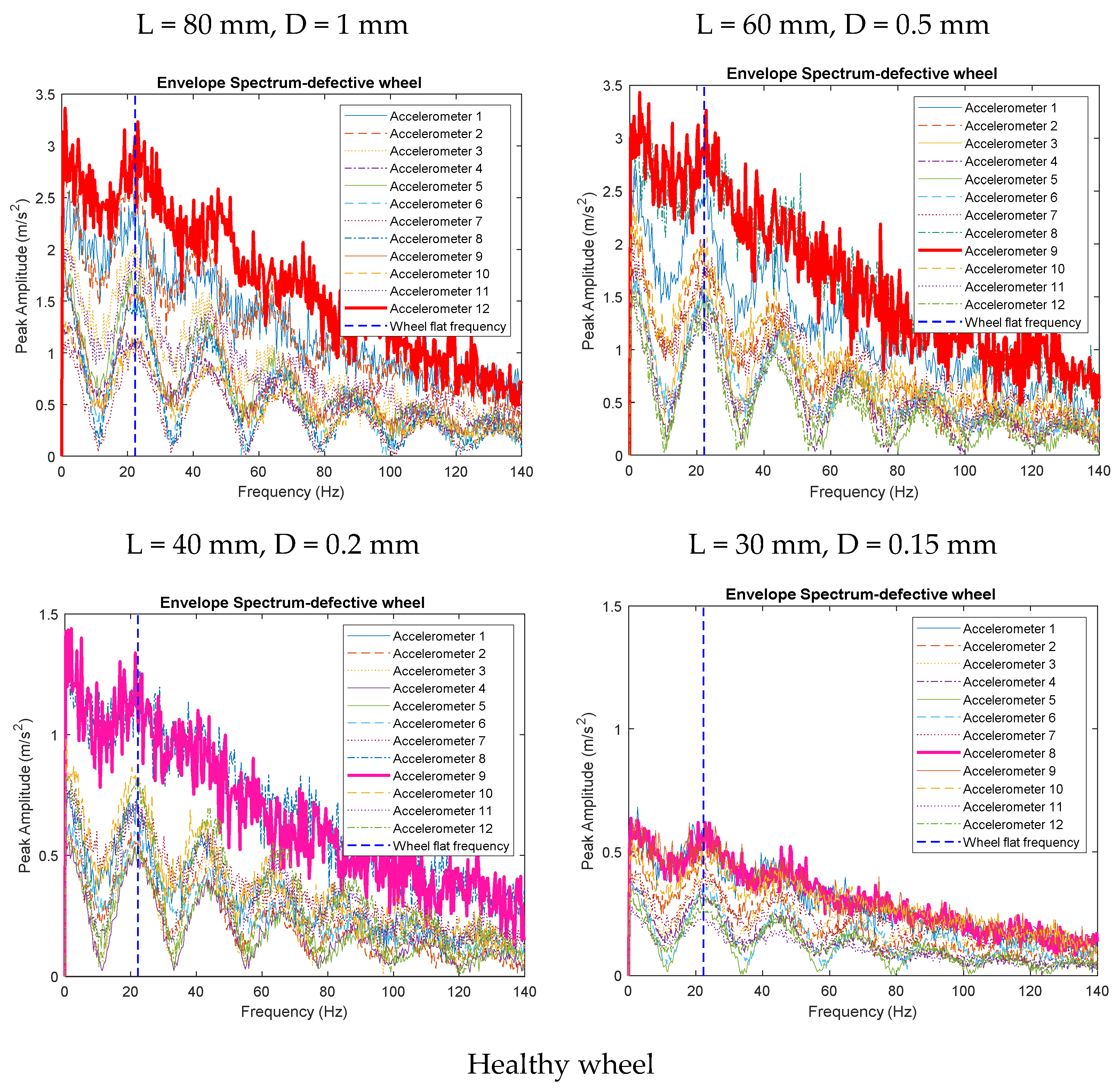
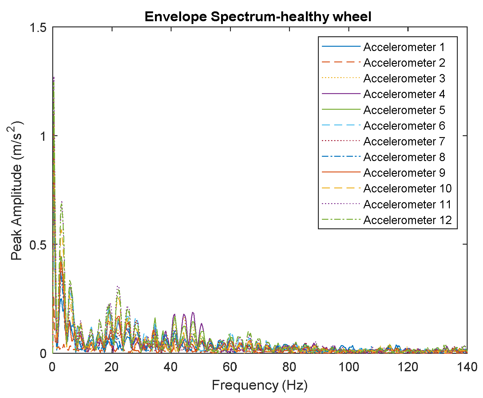
7. Sensitivity of the Layout Schemes to the Severity of the Flat

As previously stated, when the envelope spectrum analysis is carried out using acceleration signals, the amplitudes of the envelope spectrum obtained in a scenario with healthy wheels and in another with defective ones are significantly different. The amplitude of the envelope spectrum for a defective wheel is greater than for a healthy one. The present section aims to illustrate the sensitivity of the layout schemes to the severity of the flat. Hence, the influence of the flat geometry on the acceleration response is investigated in this section. In addition to the flat geometry used in the previous sections (L = 150 mm and D = 1.5 mm), other flat geometries are also considered in this section with different flat lengths (25 mm < L < 80 mm) and flat depths (0.1 mm < D < 1 mm). Moreover, signal contamination with 10% noise and the track irregularity profiles presented before are also considered in the analyses discussed in the present section.

Figure 17 shows the envelope spectrum detection analysis for 12 acceleration responses obtained on the rail (position 1 to 12 shown in Figure 5) considering a healthy and a defective wheel of the Alfa Pendular with 10% noise incorporated in the signals. Again, the layout composed by accelerometers proved to be efficient since both the lag and the amplitude indicators are suitable for distinguishing a healthy from a defective wheel, regardless of the flat geometry properties. From the results presented in the above figure, it can be concluded that the system is effective for the range of small to severe flat properties, considering a combination of noise level and rail unevenness.

8. Conclusions

This paper aimed to identify the best options regarding the type of sensors and their location in a wayside system for wheel flat detection. Based on this, a multisensory layout scheme has been proposed to detect the presence of wheel flats on both passenger and freight trains. Hence, a wheel flat recognition methodology has been developed based on simulated signals obtained with a vehicle-track interaction model. Both shear and acceleration measurement points were considered to examine the sensitivity of the layout schemes not only to the type of sensors (strain gauge and accelerometer) but also to the position where they are installed. By considering the evaluated shear and accelerations in 19 positions of the track as inputs, the wheel flat was identified by the envelope spectrum approach with spectral kurtosis analysis. The influence of the type of sensors and installation location on the accuracy of the wheel flat detection system is analyzed. Two types of trains, namely the Alfa Pendular passenger train and a freight wagon, were considered. This study allowed us to draw the following conclusions:

• The methodology proposed in this work to detect wheel flats and distinguish defective from healthy wheels is based on the envelope spectrum analysis. In this regard, extracting the impulsive signal with amplitude modulation proved a critical preprocessing step before performing the envelope spectrum. In this study, the center frequency and the bandwidth frequency of the signal were obtained first, and then this information was used as input to detect defective wheels through the envelope spectrum approach.
• In situations where the signal is significantly contaminated by noise, the use of a layout scheme composed of accelerometers is clearly more advantageous than using the strain gauges to perform an envelope spectrum to detect defective wheels. When the envelope spectrum is performed with the acceleration as input, there are significant differences in the amplitudes of the envelope spectrum response obtained in a scenario with healthy wheels and in a scenario with a defective one.
• This finding confirms the importance of kurtosis to obtain the center frequency because the impulse signal obtained with the accelerometer is more obvious than that obtained with the strain gauge. Moreover, in noised contaminated signals, the impulse signal is even more visible due to the defective wheel, and with kurtosis, the center frequency and bandwidth would be obtained more accurately.
• To detect a defective wheel, there is no need to install 12 strain gauges or accelerometers along the perimeter of a wheel since, according to the results obtained in this work, it is clear that the same results are achieved with only two accelerometers on the rail web.
• The results show that the system, regardless of the position of the sensors and the severity of the flat, is always effective in detecting wheel flats, which is a major advantage regarding the installing process.

For the final development of the proposed methodology, it is imperative to develop an automatic indicator to distinguish a defective wheel from a healthy one. Moreover, based on artificial intelligence techniques, a threshold should be defined to detect a damaged wheel. Finally, the application of the proposed method will be studied considering different speeds and unevenness profiles and tested under real field conditions by considering environmental disturbance, measurement error, and electronic interference. The optimization of the system should be thoroughly evaluated with respect to the various characteristics of wheel flats and several types of trains.

References

1. Nielsen, J.C.O.; Johansson, A. Out-of-round railway wheels-a literature survey. Proc. Inst. Mech. Eng. Part F J. Rail Rapid Transit 2000, 214, 79–91. [Google Scholar] [CrossRef]
2. Barke, D.W.; Chiu, W.K. A Review of the Effects of Out-Of-Round Wheels on Track and Vehicle Components. Proc. Inst. Mech. Eng. Part F J. Rail Rapid Transit 2005, 219, 151–175. [Google Scholar] [CrossRef]
3. Johansson, A.; Andersson, C. Out-of-round railway wheels—A study of wheel polygonalization through simulation of three-dimensional wheel–rail interaction and wear. Veh. Syst. Dyn. 2005, 43, 539–559. [Google Scholar] [CrossRef]
4. Nielsen, J. Out-of-Round Railway Wheels; Chalmers University of Technology: Göteborg, Sweden, 2009. [Google Scholar]
5. Fesharakifard, R.; Dequidt, A.; Tison, T.; Coste, O. Dynamics of railway track subjected to distributed and local out-of-round wheels. Mech. Ind. 2013, 14, 347–359. [Google Scholar] [CrossRef]
6. Lan, Q.; Dhanasekar, M.; Handoko, Y.A. Wear damage of out-of-round wheels in rail wagons under braking. Eng. Fail. Anal. 2019, 102, 170–186. [Google Scholar] [CrossRef]
7. Dukkipati, R.V.; Dong, R. Impact Loads due to Wheel Flats and Shells. Veh. Syst. Dyn. 1999, 31, 1–22. [Google Scholar] [CrossRef]
8. Wu, T.; Thompson, D. A hybrid model for the noise generation due to railway wheel flats. J. Sound Vib. 2002, 251, 115–139. [Google Scholar] [CrossRef]
9. Uzzal, R.U.A.; Ahmed, W.; Rakheja, S. Dynamic analysis of railway vehicle-track interactions due to wheel flat with a pitch-plane vehicle model. J. Mech. Eng. 2008, 39, 86–94. [Google Scholar] [CrossRef] [Green Version]
10. Vale, C. Influência da Qualidade dos Sistemas Ferroviários no Comportamento Dinâmico e no Planeamento da Manutenção Preventiva de Vias de Alta Velocidade. Ph.D. Thesis, Faculty of Engineering of the University of Porto, Porto, Portugal, 2010. (In Portuguese). [Google Scholar]
11. Li, Y.; Liu, J.; Wang, Y. Railway Wheel Flat Detection Based on Improved Empirical Mode Decomposition. Shock. Vib. 2016, 2016, 1–14. [Google Scholar] [CrossRef]
12. Alemi, A.; Corman, F.; Pang, Y.; Lodewijks, G. Reconstruction of an informative railway wheel defect signal from wheel–rail contact signals measured by multiple wayside sensors. Proc. Inst. Mech. Eng. Part F J. Rail Rapid Transit 2018, 233, 49–62. [Google Scholar] [CrossRef] [Green Version]
13. Palo, M. Condition Monitoring of Railway Vehicles, A Study on Wheel Condition for Heavy Haul Rolling Stock; Operation and Maintenance Engineering Luleå University of Technology: Luleå, Sweden, 2012. [Google Scholar]
14. Baasch, B.; Heusel, J.; Roth, M.; Neumann, T. Train Wheel Condition Monitoring via Cepstral Analysis of Axle Box Accelerations. Appl. Sci. 2021, 11, 1432. [Google Scholar] [CrossRef]
15. Song, Y.; Wang, Z.; Liu, Z.; Wang, R. A spatial coupling model to study dynamic performance of pantograph-catenary with vehicle-track excitation. Mech. Syst. Signal Process. 2021, 151, 107336. [Google Scholar] [CrossRef]
16. Luo, R. Anti-sliding control simulation of railway vehicle braking. Chin. J. Mech. Eng. 2008, 44, 35–40. [Google Scholar] [CrossRef]
17. Bosso, N.; Gugliotta, A.; Zampieri, N. Wheel flat detection algorithm for onboard diagnostic. Measurement 2018, 123, 193–202. [Google Scholar] [CrossRef]
18. Cavuto, A.; Martarelli, M.; Pandarese, G.; Revel, G.; Tomasini, E.P. Train wheel diagnostics by laser ultrasonics. Measurement 2016, 80, 99–107. [Google Scholar] [CrossRef]
19. Amini, A.; Entezami, M.; Papaelias, M. Onboard detection of railway axle bearing defects using envelope analysis of high frequency acoustic emission signals. Case Stud. Nondestruct. Test. Eval. 2016, 6, 8–16. [Google Scholar] [CrossRef] [Green Version]
20. Zhang, Z.; Entezami, M.; Stewart, E.; Roberts, C. Enhanced fault diagnosis of roller bearing elements using a combination of empirical mode decomposition and minimum entropy deconvolution. Proc. Inst. Mech. Eng. Part C J. Mech. Eng. Sci. 2015, 231, 655–671. [Google Scholar] [CrossRef]
21. Meixedo, A.; Goncalves, A.; Calcada, R.; Gabriel, J.; Fonseca, H.; Martins, R. Weighing in motion and wheel defect detection of rolling stock. In Proceedings of the 2015 3rd Experiment International Conference (exp.at’15), Ponta Delgada, Portugal, 2–4 June 2015. [Google Scholar]
22. Amini, A.; Entezami, M.; Huang, Z.; Rowshandel, H.; Papaelias, M. Wayside detection of faults in railway axle bearings using time spectral kurtosis analysis on high-frequency acoustic emission signals. Adv. Mech. Eng. 2016, 8. [Google Scholar] [CrossRef] [Green Version]
23. Colaço, A.; Costa, P.A.; Connolly, D.P. The influence of train properties on railway ground vibrations. Struct. Infrastruct. Eng. 2016, 12, 517–534. [Google Scholar] [CrossRef]
24. Mosleh, A.; Meixedo, A.; Costa, P.; Calçada, R. Trackside Monitoring Solution for Weighing in Motion of Rolling Stock. In Proceedings of the TESTE2019—2nd Conference on Testing and Experimentations in Civil Engineering—Proceedings, Porto, Portugal, 19–21 February 2019. [Google Scholar] [CrossRef]
25. Mosleh, A.; Costa, P.A.; Calçada, R. A new strategy to estimate static loads for the dynamic weighing in motion of railway vehicles. Proc. Inst. Mech. Eng. Part F J. Rail Rapid Transit 2020, 234, 183–200. [Google Scholar] [CrossRef]
26. Kouroussis, G.; Kinet, D.; Moeyaert, V.; Dupuy, J.; Caucheteur, C. Railway structure monitoring solutions using fibre Bragg grating sensors. Int. J. Rail Transp. 2016, 4, 135–150. [Google Scholar] [CrossRef]
27. Alexandrou, G.; Kouroussis, G.; Verlinden, O. A comprehensive prediction model for vehicle/track/soil dynamic response due to wheel flats. J. Rail Rapid Transit 2016, 230, 1088–1104. [Google Scholar] [CrossRef]
28. Mosleh, A.; Costa, P.; Calçada, R. Development of a Low-Cost Trackside System for Weighing in Motion and Wheel Defects Detection. Int. J. Railw. Res. 2020, 7, 1–9. [Google Scholar]
29. Stratman, B.; Yongming, L.; Sankaran, M. Structural Health Monitoring of Railroad Wheels Using Wheel Impact Load Detectors. J. Fail. Anal. Preven. 2007, 7, 218–225. [Google Scholar] [CrossRef]
30. Liu, X.; Ni, Y. Wheel tread defect detection for high-speed trains using FBG-based online monitoring techniques. Smart Struct. Syst. 2018, 21, 687–694. [Google Scholar]
31. Gao, R.; He, Q.; Feng, Q. Railway Wheel Flat Detection System Based on a Parallelogram Mechanism. Sensors 2019, 19, 3614. [Google Scholar] [CrossRef] [Green Version]
32. Liang, M.; Bozchalooi, I.S. An energy operator approach to joint application of amplitude and frequency-demodulations for bearing fault detection. Mech. Syst. Signal Process. 2010, 24, 1473–1494. [Google Scholar] [CrossRef]
33. Zhou, C.; Gao, L.; Xiao, H.; Hou, B. Railway Wheel Flat Recognition and Precise Positioning Method Based on Multisensor Arrays. Appl. Sci. 2020, 10, 1297. [Google Scholar] [CrossRef] [Green Version]
34. Merainani, B.; Benazzouz, D.; Rahmoune, C. Early detection of tooth crack damage in gearbox using empirical wavelet transform combined by Hilbert transform. J. Vib. Control. 2017, 23, 1623–1634. [Google Scholar] [CrossRef]
35. Lv, Y.; Ge, M.; Zhang, Y.; Yi, C.; Ma, Y. A Novel Demodulation Analysis Technique for Bearing Fault Diagnosis via Energy Separation and Local Low-Rank Matrix Approximation. Sensors 2019, 19, 3755. [Google Scholar] [CrossRef] [Green Version]
36. Meixedo, A.; Goncalves, A.; Calcada, R.; Gabriel, J.; Fonseca, H.; Martins, R. On-line monitoring system for tracks. In Proceedings of the 3rd Experiment International Conference: Online Experimentation, Ponta Delgada, Portugal, 2–4 June 2015. [Google Scholar]
37. Mosleh, A.; Montenegro, P.; Costa, P.A.; Calçada, R. An approach for wheel flat detection of railway train wheels using envelope spectrum analysis. Struct. Infrastruct. Eng. 2020, 1–20. [Google Scholar] [CrossRef]
38. ANSYS®. Academic Research, Release 19.2; ANSYS Inc.: Canonsburg, PA, USA, 2018. [Google Scholar]
39. Neto, J.; Montenegro, P.A.; Vale, C.; Calçada, R. Evaluation of the train running safety under crosswinds—A numerical study on the influence of the wind speed and orientation considering the normative Chinese hat model International. J. Rail Transp. 2020, 1–28. [Google Scholar] [CrossRef]
40. Neto, J.; Montenegro, P.A.; Calçada, R. An innovative approach for an inverse dynamic model of a freight wagon. In Proceedings of the 1st International Symposium on Risk Analysis and Safety of Complex Structures and Components, Porto, Portugal, 1–2 July 2019. [Google Scholar]
41. European Standard. Railway Applications Railway Applications—Track-Rail-Part1: Vignole Railway 46 kg/m and above; peEN 13674–1, Final Draft; European Union: Brussels, Belgium, 2002. [Google Scholar]
42. Zhai, W.; Wang, K.; Cai, C. Fundamentals of vehicle-track coupled dynamics. Veh. Syst. Dyn. 2009, 47, 1349–1376. [Google Scholar] [CrossRef]
43. ERRI D 214/RP 5. Rail Bridges for Speeds > 200 km/h: NUMERICAL Investigation of the Effect of Track Irregularities at Bridge Resonance; European Rail Research Institute: Utrecht, The Netherlands, 1999. [Google Scholar]
44. UIC 774-3-R. Track/Bridge Interaction—Recommendations for Calculation, 2nd ed.; International Union of Railways (UIC): Paris, France, 2001. [Google Scholar]
45. Wu, Y.D.; Yang, Y.B. Steady-state response and riding comfort of trains moving over a series of simply supported bridges. Eng. Struct. 2003, 25, 251–265. [Google Scholar] [CrossRef]
46. ERRI D 202/RP 11. Improved Knowledge of Forces in CWR Track (Including Switches): Parametric Study and Sensivity Analysis of Cwerri; European Rail Research Institute: Utrecht, The Netherlands, 1999. [Google Scholar]
47. Auersch, L. Dynamic interaction of various beams with the underlying soil—Finite and infinite, half-space and Winkler models. Eur. J. Mech. A/Solids 2008, 27, 933–958. [Google Scholar] [CrossRef]
48. Neves, S.; Montenegro, P.; Azevedo, A.; Calçada, R. A direct method for analyzing the nonlinear vehicle–structure interaction. Eng. Struct. 2014, 69, 83–89. [Google Scholar] [CrossRef] [Green Version]
49. Montenegro, P.A.; Neves, S.G.M.; Azevedo, A.F.M.; Calçada, R. A nonlinear vehicle-structure interaction methodology with wheel-rail detachment and reattachment. In Proceedings of the COMPDYN 2013—4th ECCOMAS Thematic Conference on Computational Methods in Structural Dynamics and Earthquake Engineering, Kos, Greece, 12–14 June 2013. [Google Scholar]
50. Neves, S.; Azevedo, A.; Calçada, R. A direct method for analyzing the vertical vehicle–structure interaction. Eng. Struct. 2012, 34, 414–420. [Google Scholar] [CrossRef] [Green Version]
51. Montenegro, P.; Neves, S.; Calçada, R.; Tanabe, M.; Sogabe, M. Wheel-rail contact formulation for analyzing the lateral train-structure dynamic interaction. Comput. Struct. 2015, 152, 200–214. [Google Scholar] [CrossRef] [Green Version]
52. Hertz, H. Ueber die Berührung fester elastischer Körper [On the contact of elastic solids]. J. Reine Angew. Math. 1882, 92, 156–171. [Google Scholar]
53. Kalker, J.J. Book of Tables for the Hertzian Creep-Force Law; Delft University of Technology: Budapest, Hungary, 1996. [Google Scholar]
54. MATLAB®. Release R2018a; The MathWorks Inc.: Natick, MA, USA, 2018. [Google Scholar]
55. Montenegro, P.A. A Methodology for the Assessment of the Train Running Safety on Bridges; Faculty of Engineering of the University of Porto: Porto, Portugal, 2015. [Google Scholar]
56. Abell, M.L.; Braselton, J.P.; Rafter, J.A. Statistics with Mathematica; Academic Press: New York, NY, USA, 1999. [Google Scholar]
57. Brandt, A. Noise and Vibration Analysis: Signal Analysis and Experimental Procedures; John Wiley & Sons: New York, NY, USA, 2011. [Google Scholar]
58. Entezami, M.; Roberts, C.; Weston, P.; Stewart, E.; Amini, A.; Papaelias, M. Perspectives on railway axle bearing condition monitoring. Proc. Inst. Mech. Eng. Part F J. Rail Rapid Transit 2019, 234, 17–31. [Google Scholar] [CrossRef]
59. Hasan, T. Complex Demodulation: Some Theory and Applications. Handb. Stat. 1983, 3, 125–156. [Google Scholar]
60. Antoni, J. Fast computation of the kurtogram for the detection of transient faults. Mech. Syst. Signal Process. 2007, 21, 108–124. [Google Scholar] [CrossRef]
61. Antoni, J. The spectral kurtosis: A useful tool for characterising non-stationary signals. Mech. Syst. Signal Process. 2006, 20, 282–307. [Google Scholar] [CrossRef]
Figure 1. Dynamic models of the railway vehicles: lateral views of the (a) Alfa Pendular and (b) freight wagon, and front views of the (c) Alfa Pendular and (d) freight wagon.
Applsci 11 04002 g001aApplsci 11 04002 g001b
Figure 2. Railway track modeling.
Applsci 11 04002 g002
Figure 3. Track irregularity sample: (a) vertical and (b) lateral direction.
Applsci 11 04002 g003
Figure 4. The modeling of train-track interaction.
Applsci 11 04002 g004
Figure 5. Schematic of a vehicle containing the damaged wheel.
Applsci 11 04002 g005
Figure 6. The methodology to identify a defective wheel.
Applsci 11 04002 g006
Figure 7. Framework to obtain the kurtogram, the central frequency, and the frequency band for each signal.
Applsci 11 04002 g007
Figure 8. (a): Main signal evaluated from position 9 regarding layout scheme 1. (b): Spectral kurtosis for a signal corresponding to the Alfa Pendular train, Kmax = 60.25 Hz, optimal window length = 16, center frequency = 0.1875 kHz, bandwidth frequency = 0.125 kHz.
Applsci 11 04002 g008
Figure 9. Envelope spectrum analysis for the 12 strain gauges (layout scheme 1) for the Alfa Pendular and the freight wagon, considering the unevenness profile of the track, (a) a defective wheel Alfa Pendular, (b) a healthy wheel Alfa Pendular, (c) a defective wheel freight wagon, and (d) a healthy wheel freight wagon.
Applsci 11 04002 g009
Figure 10. Kurtosis values for healthy and defective wheels corresponding to 12 positions of the strain gauges for the passage of the Alfa Pendular.
Applsci 11 04002 g010
Figure 11. Envelope spectrum analysis for the 12 accelerometers (layout scheme 2) for the Alfa Pendular and the freight wagon, considering the unevenness profile of the track for (a) a defective wheel Alfa Pendular, (b) a healthy wheel Alfa Pendular, (c) a defective wheel freight wagon, and (d) a healthy wheel freight wagon.
Applsci 11 04002 g011
Figure 12. Envelope spectrum analysis for the 12 strain gauges (layout scheme 1) with different noise intensities and considering a defective and healthy wheel of the Alfa Pendular train and the freight wagon.
Applsci 11 04002 g012
Figure 13. Envelope spectrum analysis for the 12 accelerometers (layout scheme 2) with different noise intensities and considering a defective and healthy wheel of the Alfa Pendular train and the freight wagon.
Applsci 11 04002 g013
Figure 14. Kurtosis values for signals with and without noise for the Alfa Pendular passage for layout scheme 2.
Applsci 11 04002 g014
Figure 15. Envelope spectrum analysis for seven accelerometers (layout scheme 3) considering a defective and a healthy wheel of the Alfa Pendular and the freight wagon (noise = 10%).
Applsci 11 04002 g015aApplsci 11 04002 g015b
Figure 16. Optimization of the sensor layout.
Applsci 11 04002 g016
Figure 17. Envelope spectrum analysis for 12 accelerometers (layout scheme 2) considering a defective and a healthy wheel of the Alfa Pendular due to the severity of the flat considering 10% noise.
Applsci 11 04002 g017aApplsci 11 04002 g017b